Ant Colony Optimization for Accelerated Pathway Identification in Connection Element Method Reservoir Models: A Fast-Track Solution for Large-Scale Simulations

Abstract

In recent years, reservoir models based on the Connection Element Method (CEM) have gained extensive application in reservoir development. This mesh-free modeling approach effectively captures all flow paths and flow-splitting coefficients between nodes, providing a clear view of flow interactions and accurately identifying primary connectivity pathways between injection and production wells. However, the traditional approach of traversing flow paths and splitting coefficients imposes a significant computational load, particularly when applied to large reservoirs with numerous virtual wells. To enhance simulation efficiency, this paper introduces a novel method leveraging the Ant Colony Optimization (ACO) algorithm to efficiently identify the path with the highest splitting coefficient between well pairs. This approach rapidly calculates and filters the dominant connectivity paths between injection and production wells in CEM models. A comparative analysis shows that, while the ACO algorithm provides limited benefit with a small number of connectivity paths, it significantly outperforms the conventional depth-first search algorithm as the number of experimental wells increases.

1. Introduction

In reservoir numerical simulation models, finite difference methods [1,2], finite volume methods [3,4,5], and finite element methods [6,7] are widely employed for conducting flow simulation calculations. These methodologies rely on a grid topology [8] that segments the computational domain of the reservoir and defines connectivity relationships between grid cells through grid topological structures. These methods calculate the associated transmissibility and formulate computational connection tables [9]. The fundamental focus of conventional reservoir numerical simulation models predominantly involves the development of connection tables and associated conductance coefficients between well grid cells, grounded in grid topological structures. Nevertheless, the intrinsic constraints of these grid topological structures impede their capacity to precisely assess and compute connectivity coefficients in complex reservoir models. This limitation is particularly pronounced in highly intricate reservoir environments, where the construction and generation of grid topologies become exceedingly challenging [10,11]. To address these inherent limitations, a novel reservoir simulation model, termed the Connectivity Element Method (CEM), has been proposed. CEM employs a meshless node-based representation [12] to effectively overcome the constraints encountered by traditional models in complex geological settings. By capitalizing on its inherent flexibility, CEM transforms the intricate multidimensional flow coupling calculations [13] into simplified one-dimensional flow parallel calculations [14]. This transformation facilitates the creation of more diverse connectivity relationships while maintaining the integrity of flow structures between wells.

The adaptability of the CEM reservoir model facilitates a more intuitive comprehension of flow interactions among wells or nodes. By monitoring all flow paths [15] and the flow splitting coefficients [16] between nodes, it becomes feasible to identify the predominant flow paths [17]. The splitting coefficient represents the distribution of injected fluid [18] along a particular flow path. Typically, when the splitting coefficients of flow paths between injection and production wells are comparable, it suggests a balanced subsurface displacement. Conversely, a markedly higher splitting coefficient along a specific trajectory indicates the existence of a preferential channel [19]. Consequently, investigating advantageous pathways assumes considerable importance. In practical applications, reservoir models typically encompass numerous wells and nodes, characterized by intricate distributions of flow paths for each injection well, thereby rendering the identification and tracking of advantageous paths particularly challenging.

In contemporary reservoir modeling, the predominant method for optimal path tracking is grounded in directed graph theory [20], which entails identifying all potential flow paths from injection wells to production wells. Breadth-First Search (BFS) [21] and Depth-First Search (DFS) [22] are recognized as the most basic and intuitive search techniques within this framework. Nevertheless, as highlighted by previous research [23,24], these algorithms encounter substantial difficulties in complex models characterized by a significant increase in the number of nodes and edges, leading to a marked escalation in their computational time complexity. Furthermore, due to the intrinsic nature of BFS and DFS, which do not incorporate weights, these algorithms are limited in their capacity to address the optimization problems examined in this study. They must first generate all possible paths before subsequently considering weights specific to the problem at hand.

In recent years, the advancement of swarm intelligence algorithms has yielded significant achievements across various domains [25,26]. Notably, the adaptive pheromone adjustment Ant Colony Optimization, introduced by Gang-Li Qin and Jia-Ben Yang [27], presents a more adaptable methodology for path planning in large-scale data environments. This algorithm’s distinctive pheromone decision-making mechanism substantially decreases the time complexity associated with path planning. Consequently, this study proposes the utilization of the adaptive pheromone adjustment Ant Colony Optimization to enhance path tracking and optimization.

In the context of advantageous path searching utilizing the Ant Colony Optimization (ACO) algorithm [28], the traditional exhaustive traversal method for identifying optimal paths is supplanted by iterative searches employing the ACO algorithm to identify paths that satisfy the specified criteria. By foregoing the DFS full traversal, which exhibits an exponential increase in time complexity relative to the number of nodes [29], the computational time and power consumption are significantly diminished. Consequently, this approach expedites the overall process of advantageous path tracking.

An examination of the practical applications of the ACO algorithm across diverse disciplines—such as developing transmission strategies in wireless sensor networks [30], resolving network routing issues [31], and planning paths for unmanned vessels [32]—demonstrates that ACO, as a swarm intelligence algorithm, serves as a robust optimization mechanism for addressing discrete optimization challenges in engineering domains. With the ongoing advancements in intelligent algorithms, ACO has attracted increasing scholarly attention and has been successfully applied in numerous contexts. Extensive theoretical and empirical achievements provide effective guidelines for its application. Experimental findings indicate that ACO exhibits exceptional computational efficiency and strategic adaptability, particularly in optimizing advantageous paths within complex geological models, including unstructured grid-connected reservoir models.

This is particularly true concerning computational efficiency and strategic adaptability. Within the ACO framework, pheromones play a crucial role in node selection and decision-making processes, with the probability of selection being affected by both the path weights and pheromone concentrations. These parameters can be fine-tuned by adjusting the coefficients α and β [33], alongside other influencing factors [34]. According to researchers who have enhanced ACO algorithms to meet specific requirements [35,36,37], the optimal path identified through ACO demonstrates an ability to adapt its strategy in response to changing conditions, thereby providing a level of flexibility that traditional exhaustive tracking methods cannot match.

The primary aim of this study is to enhance the optimization of advantageous path tracking in complex reservoir models through the application of the ACO algorithm, specifically addressing the challenge of slow computational speed encountered in practical production scenarios. Section 2 presents the fundamental principles of advantageous path tracking and the ACO algorithm, followed by modifications to the heuristic function of the ACO algorithm to enable its application to the advantageous path tracking problem. In Section 3, the feasibility of the proposed ACO-based optimization algorithm is validated using two real-world models. Section 4 involves a comparative analysis of multiple sets of experimental well points of varying sizes. The study ultimately concludes that, within complex reservoir models, the ACO algorithm exhibits superior computational speed and stability, effectively mitigating the issue of slow computation speed associated with conventional algorithms in such contexts.

2. Indicators Between Injection and Production Wells and Basic Principles of Ant Colony Optimization

2.1. Injection–Production Splitting Coefficient

The implementation of a meshless well model within the CEM facilitates a more intuitive and precise evaluation of the flow interactions between wells and nodes. To accurately assess these interactions, we assume that, at the n-th time step, the upstream node a is directly connected to the downstream node b through a unit connection element. The splitting coefficient for the simple path a−b is defined as:

$${\lambda }_{a, b}^n={\displaystyle \frac{q_{a,b}^n}{{{\displaystyle \sum }}_{k=1}^{n_c^a}{q}_{i,k}^n}}$$

(1)

In Equation (1), $n_c^a$ is the number of downstream nodes connected to node a, and $q_{a,b}^n$ represents the flow rate through the connection element between nodes a and b at the n-th time step. The denominator is the total flow rate of all connection elements between node a and its downstream nodes at the n-th time step.

Equation (1) indicates the proportion of the flow rate through the specific connection element relative to the total flow rate through all connection elements between node a and its downstream nodes.

To elucidate the complete procedure for determining splitting coefficients, an illustrative example is presented, grounded in a specific model connection diagram. The data depicted in this diagram are extracted from a hypothetical model, which is constructed using assumed values extrapolated from real-world data. This model is designed exclusively to offer a comprehensive demonstration of the methodology involved in solving splitting coefficients.

As shown in Figure 1, which illustrates the inter-well flow connectivity of an equilateral triangle model, the orange circles represent injection wells, the yellow circles represent production wells, and the blue circles represent virtual wells. The direction of the arrows indicates the direction of fluid flow, with each line segment representing a connection element. The data on each connection element correspond to the flow rate between wells. Each well is assigned a number, and the value in parentheses after each number denotes the current pressure of that well.

In Figure 1, the flow rates between connection elements and the pressure at each well are determined using reservoir numerical simulation software based on the CEM. The underlying calculation methodology is as follows: each connection element is characterized by two primary indicators—conductivity and connected volume—which represent the efficiency of fluid transfer and the spatial capacity of the connection element, respectively. By formulating a multi-layer reservoir material balance equation, a mathematical model is developed to compute the pressure at each well at a specific time. By integrating the conductivity between well points with the calculated pressure differentials, the fluid flow rates within the connection elements, as depicted in Figure 1, can be further ascertained.

Based on Equation (1), the splitting coefficient of each connection element can be calculated. Taking virtual well 7 as an example, which is connected to wells 1, 3, and 6, the flow directions indicated by the arrows in the figure show that well 7 only flows towards wells 3 and 6. Accordingly, the splitting coefficient of the connection element from well 7 to well 3 can be determined.

$${\lambda }_{3,7}={\displaystyle \frac{8.574}{1.904+8.574}}=0.818$$

(2)

In this case, 8.574 represents the inter-well flow rate between connection elements 3 and 7, while 1.904 represents the inter-well flow rate between well 7 and well 6. The denominator is the sum of the inter-well flow rates from well 7 to wells 3 and 6, and the numerator is the inter-well flow rate of the target connection elements 3 and 7. As shown in the formula, the splitting coefficient of connection elements 3 and 7 is calculated to be 0.818. By following this approach, the splitting coefficient for each connection element in the equilateral triangle model can be calculated sequentially. Figure 2 displays all the splitting coefficients for each unit as determined through these calculations.

After obtaining the splitting coefficients for all connection elements in the equilateral triangle model, starting from the injection well (well 1) and ending at the production wells (wells 2 and 3), many paths can be traced based on the flow directions between wells. For example, considering the path from well 1 to well 2, specifically the path {1, 4, 6, 2}, the splitting coefficient of this path can be determined by combining the splitting coefficients of the individual connection elements along this path, as calculated in Figure 2. The calculation results are as follows:

$${\lambda }_{1,2}^{n,1}={\lambda }_{1,4}^{n,1}\times {\lambda }_{4,6}^{n,1}\times {\lambda }_{6,2}^{n,1}=0.413\times 0.077\times 0.476=0.015$$

(3)

Equation (3) represents the calculation of the overall splitting coefficient for a path. The splitting coefficient of the path from well point 1 to well point 2 is the product of the splitting coefficients of all individual segments that compose the path. For example, consider the path {1, 4, 6, 2} from well point 1 to well point 2. The splitting coefficient for this path is obtained by multiplying the splitting coefficients of the segments between well points 1 and 4, 4 and 6, and 6 and 2.

A directed sequence originating from the injection well and terminating at the production well delineates a pathway, signifying the movement of fluid from a region of higher pressure to one of lower pressure. The sequence {1, 4, 6, 2}, as previously computed, exemplifies such a pathway, with Figure 3 offering a comprehensive depiction of this particular route.

2.2. Ant Colony Optimization Principle

The ACO is an algorithmic approach for optimization, drawing inspiration from the foraging behavior of ants to address path-planning challenges.

In this algorithm, let the total number of ants be i. Ants use pheromones to determine the selection of the next node. The probability $p_{n,m}^k\left(t\right)$ that ant k will transition from node n to the subsequent node m is defined by:

$$p_{n,m}^k\left(t\right)=\left\{\begin{array}{c}{\displaystyle \frac{{\left[{\tau }_{n,m}\left(t\right)\right]}^{\alpha }{\left[{\eta }_{n,m}\left(t\right)\right]}^{\beta }}{\sum u\in M_k{\left[{\tau }_{n,u}\left(t\right)\right]}^{\alpha }{\left[{\eta }_{n,u}\left(t\right)\right]}^{\beta }}} ,m\in M_k\\ 0 ,otherwise\end{array}\right.$$

(4)

$M_k$ represents the set of paths traversed by the ant k during one iteration. $u\in M_k$ represents all possible candidate nodes, and $u$ serves as a traversal variable in this formula to summarize the contribution of information from all candidate nodes to the transition probability.

In the computational strategy of the algorithm, the parameters α and β play critical roles. Specifically, α represents the pheromone factor, whereas β denotes the heuristic information factor.

Heuristic information functions as supplementary data that impacts the decision-making processes of ants, facilitating their selection of more optimal paths and thereby expediting the identification of the optimal solution to a particular problem. In the classical traveling salesman problem, heuristic information might encompass the distances between paths, encouraging ants to prefer shorter routes. In optimization problems, heuristic information may include attributes such as productivity or cost. In the context of the advantageous path-tracking problem examined in this study, the heuristic information is represented by the unit-splitting coefficient, which will be elaborated upon in the subsequent subsection. This subsection is dedicated exclusively to discussing the foundational implementation principles of the ant colony algorithm.

These parameters are pre-set according to the model to balance the influence of heuristic information and pheromone concentration. When α = 0, the algorithm simplifies to a traditional random greedy algorithm, where nodes with larger heuristic values are more likely to be chosen, potentially leading to local optima. Conversely, when β = 0, ants rely solely on pheromone concentration to determine paths, which causes the algorithm to become a rapidly converging positive feedback system. This often results in optimal paths that significantly deviate from the actual target, leading to poor performance.

In this context, ${\tau }_{n,m}\left(t\right)$ represents the pheromone level from node n to node m at time t. ${\eta }_{n,m}\left(t\right)$ represents the heuristic function from node n to node m at time t. The ACO is typically used to solve shortest-path problems, so the heuristic function is generally denoted by ${\displaystyle \frac{1}{d_{m,n}}}$. However, since assessing advantageous paths is not simply a matter of summing shortest-path weights, detailed information about the heuristic function will be provided in the next subsection.

The pheromone level on each connection segment is updated iteratively after each generation of ants has visited all nodes. The pheromone update formula is as follows:

$${\tau }_{n,m}\left(t+1\right)=\left(1-\rho \right){\tau }_{n,m}\left(t\right)+∆{\tau }_{n,m}$$

(5)

where ρ represents the pheromone evaporation coefficient, it plays a crucial role in preventing pheromone levels from becoming excessively elevated, which could otherwise adversely impact the convergence speed and accuracy of the ACO algorithm.

The pheromone evaporation coefficient ρ determines how exploration and exploitation are balanced during the computation process. The larger the value of ρ, the faster the pheromone decays, and, vice versa, the slower the decay. By restricting ρ to a range between 0 and 1, it is possible to avoid the complete disappearance or excessive accumulation of pheromones, thus maintaining the dynamic balance of the ants’ exploration process.

When the parameter ρ is small, the evaporation rate diminishes, potentially resulting in inadequate exploration capabilities and an elevated risk of convergence to a local optimum. Conversely, a large ρ value leads to an increased evaporation rate, thereby accelerating the frequency of pheromone updates. This enhancement in pheromone dynamics facilitates more robust exploration, enabling ants to investigate new paths more frequently. In the context of the model examined in this study, the ACO algorithm consistently employs a relatively high value of ρ, specifically ρ = 0.8. This choice effectively accelerates the exploration process while augmenting the algorithm’s exploratory capacity, thereby ensuring its accuracy and reliability.

$∆{\tau }_{n,m}$ is the pheromone increment for the route from node n to node m:

$$∆{\tau }_{n,m}={\displaystyle \sum }_{k=1}^i∆{\tau }_{n,m}^k$$

(6)

This formula calculates the total pheromone deposited on the path from node n to node m by all ants. Here, $∆{\tau }_{n,m}^k$ represents the amount of pheromone released by ant k on the path from n to m. The increment in pheromone concentration is determined by the following formula:

$$∆{\tau }_{n,m}^k\left\{\begin{array}{c}{\displaystyle \frac{Q}{L_k}} ,tour\left(n,m\right)\in tou{r}_k\\ 0 ,otherwise\end{array}\right.$$

(7)

Q is the pheromone enhancement coefficient. The enhancement coefficient is a parameter related to the pheromone-update mechanism, which is used to control the degree of reward for high-quality paths during the optimization process. A larger Q value may lead to premature convergence, preventing the discovery of the optimal solution. Conversely, a smaller Q value delays the reinforcement of pheromones, increasing exploration but resulting in slower convergence. $L_k$ is the total path length traveled by ant k. Since the ACO algorithm primarily addresses the shortest-path problem, the pheromone concentration calculation ensures that shorter paths have higher concentrations. $tour$ represents a single route completed by an ant, so $tour\left(n,m\right)$ represents the route taken by an ant from node n to node m. $tou{r}_k$ represents the set of paths traversed by ant k in the current iteration, including all the visited edges. For the advantageous path analysis discussed in this paper, a detailed explanation will be provided in the next subsection.

Before the first round of ants completes their visits, the initial pheromone levels at all nodes are equal. After each round of visits is completed, the pheromone on the path is updated, with the increase in pheromone amount calculated using Equation (6). Meanwhile, considering the evaporation of pheromones over time, the final pheromone amount is calculated using Equation (5). As indicated by Equation (4), the probability of an ant selecting the next node is influenced by the values of the heuristic function and the updated pheromone. Adjusting the corresponding computation strategy factors allows the algorithm to achieve a state that is best suited to the current model. Once all iterations are completed, the optimal solution is obtained.

2.3. Advantageous Path Tracking Based on Ant Colony Optimization

In reservoir numerical simulation models utilizing the CEM, target properties can be numerically simulated based on the fundamental characteristics of well points. The outcomes of the simulation are shown in a table format, with each row containing three components: the starting node of the connected unit, the ending node, and the target property of the connected unit. The ultimate simulation results are visualized as a connectivity graph within numerical simulation software. The splitting coefficient mentioned in this paper is also derived using this method.

During the reservoir numerical simulation process, the splitting coefficient is predominantly utilized to identify optimal pathways. Conventional reservoir numerical simulations implement the DFS algorithm, which constructs a logical connectivity graph derived from the simulation data, explores all potential paths, and computes the cumulative splitting coefficient for each path. The path exhibiting the highest cumulative splitting coefficient is designated as the optimal pathway within the model. Nonetheless, in practical applications, the traditional DFS algorithm demonstrates suboptimal computational efficiency when applied to large-scale reservoirs.

As discussed in the preceding subsection, the ACO algorithm is primarily designed to address shortest-path-planning problems. Consequently, this study substitutes the conventional DFS algorithm with the ACO algorithm within the context of reservoir numerical simulation to enhance computational efficiency. The subsequent section elaborates on the specific implementation of the ACO algorithm for advantageous path tracking.

As indicated by Equation (3), identifying the optimal pathway from the injection well to the production well necessitates an assessment of the connectivity properties between each point within the reservoir model, with particular emphasis on the unit-splitting coefficient. By computing the splitting coefficients for each interconnected unit along the pathway from the injection to the production well, the cumulative splitting coefficient for the entire path can be determined. Subsequently, the cumulative splitting coefficients for all potential pathways between the injection and production wells are calculated. The pathway exhibiting the highest cumulative splitting coefficient is designated as the optimal path. Therefore, the heuristic function can be directly set to the value of the unit-splitting coefficient, specifically:

$${\eta }_{n,m}\left(t\right)={\lambda }_{n,m}$$

(8)

Incorporating the splitting coefficient of each connected unit as the heuristic value within the Ant Colony Optimization algorithm enhances its applicability to the problem of identifying optimal pathways in reservoir environments. The splitting coefficient serves as a direct metric of inter-well flow, thereby accurately representing flow dynamics within the reservoir model and more effectively directing the search for optimal paths. Furthermore, since the splitting coefficient is computed based on fundamental physical properties such as pressure and permeability, it is grounded in objective principles, thereby ensuring a high degree of reliability.

For the pheromone release concentration, it is necessary to ensure that paths with higher total splitting coefficients have higher pheromone concentrations. Thus, the pheromone concentration is defined as:

$$∆{\tau }_{n,m}^k\left\{\begin{array}{c}Q\times {\lambda }_{k ,tour\left(n,m\right)\in tou{r}_k}\\ 0 ,otherwise\end{array}\right.$$

(9)

where ${\lambda }_k$ is the total splitting coefficient of the entire path. $tour$ and $Q$ have the same meaning as in Equation (7).

Based on the above formulas and calculation steps, the overall flowchart for Advantageous Path Tracking using the Ant Colony Optimization algorithm (as shown in Figure 4) and the pseudocode can be obtained.

The pseudocode for the implementation of the Ant Colony Optimization Algorithm 1 is as follows:

Algorithm 1: Ant Colony Optimization for Tracking Advantageous Paths

Input: Connection information and splitting coefficients between well points Output: Advantageous path from the injection well to the target production well Initialize the directed graph with weighted connections between the well points; Set the parameters for the Ant Colony Optimization algorithm; Initialize the pheromone level for each connection segment; for n = 1 to the specified number of iterations do   for each ant in the colony do     Set the current well number to the designated injection well;     While i≠ the target production well, do      Choose the next node i based on the pheromone levels and heuristic function;      Record the path segment (i,j);      Update i = j;    Record and compare the score of the path (i,j);    Update the optimal path and the pheromone table;   Increment n by 1; Output the optimal path;

3. Analysis of Advantageous Path Examples

Due to the complexity of actual geological models, where injection wells and production wells are not unique and the flow paths are complex, this experiment will focus on analyzing a representative pair of injection and production wells and their connected paths. For instance, in Example 1, we analyze the advantageous path from I0 to P5. For all examples, a comparison of time complexity will be made between the traditional DFS algorithm and the ACO algorithm introduced in this paper to reach conclusions.

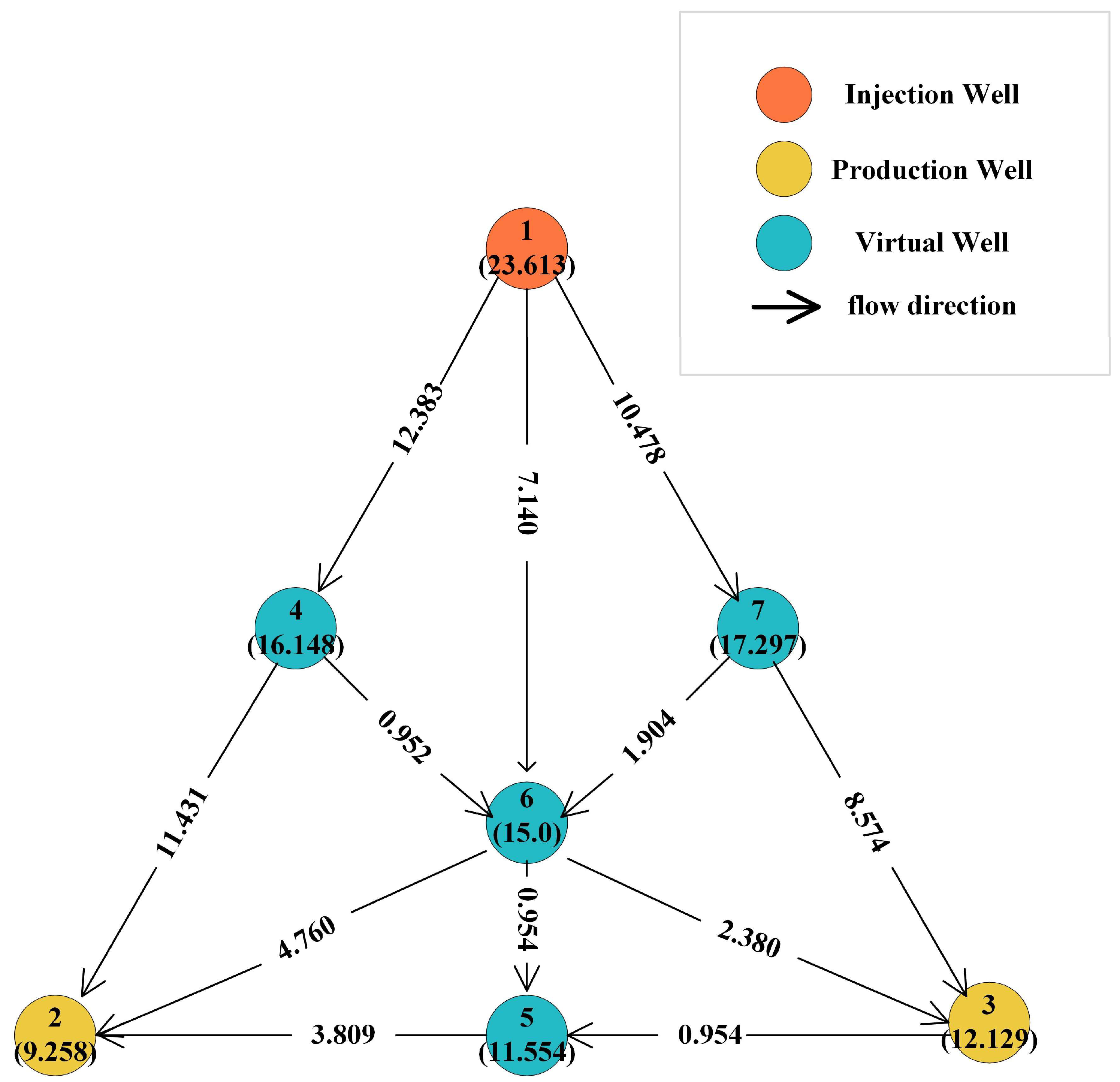
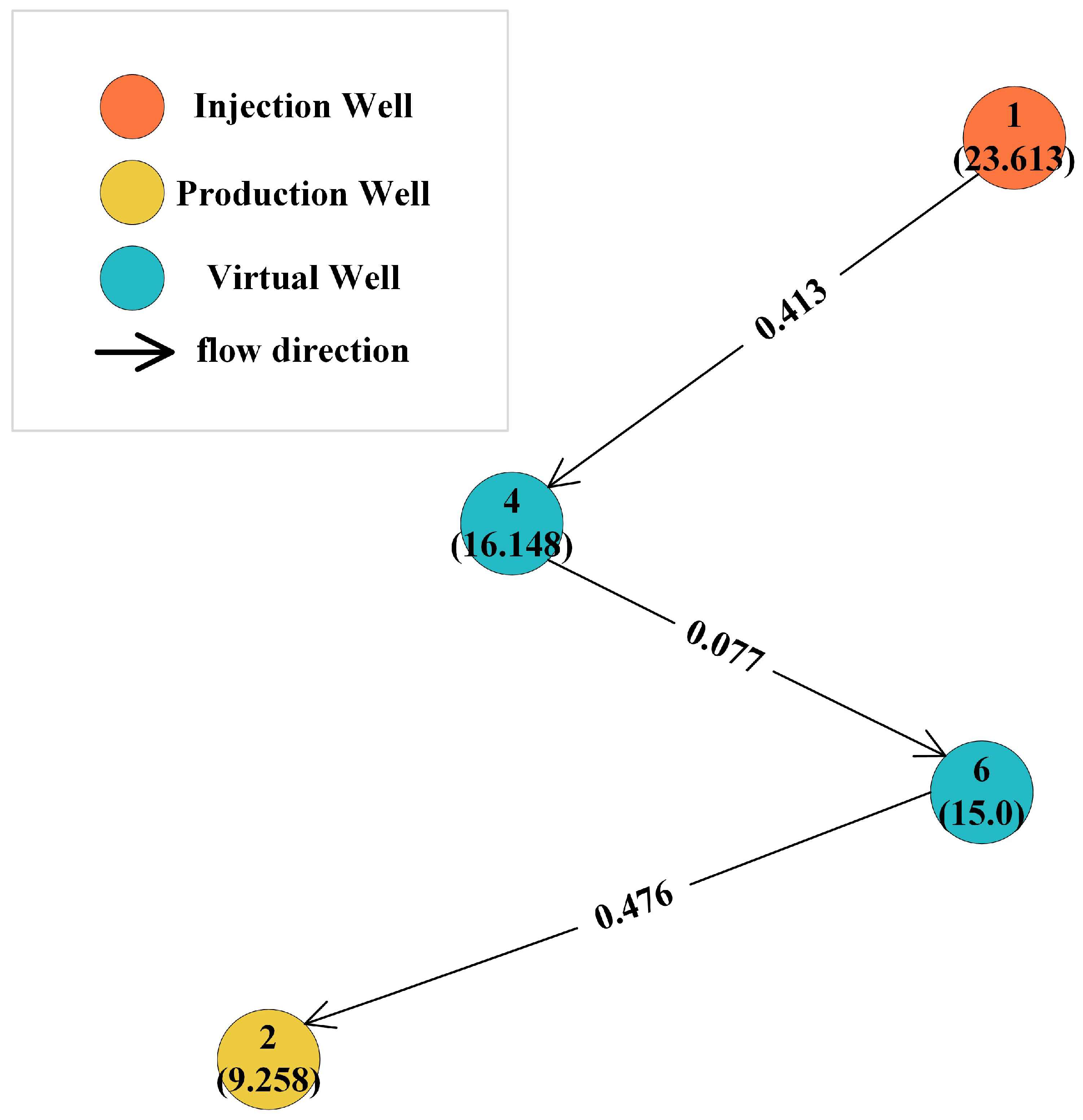
3.1. Example Model 1 of Actual Connected Well Points

In this subsection, utilizing a small oil field model comprising nine actual wells and several virtual nodes derived from a real production process, two wells have been selected for analytical and comparative experimentation. The unstructured model of this oil field, along with the connectivity diagram illustrating the interconnections between its nodes, is presented in Figure 5.

In Figure 5, the red points represent injection wells, while the white points represent production wells. The connecting lines between well points indicate the splitting coefficients of the connected units between the two wells.

The splitting coefficients for each pair of well points are determined utilizing a reservoir numerical simulation software grounded in the CEM. These software processes input data comprising the properties of each well, including pressure, permeability, and other essential characteristics obtained from the actual oil field, to compute the inter-well flow rates. Furthermore, by analyzing the pressure differentials among the wells, the flow paths of oil and gas are ascertained, indicating movement from wells with higher pressure to those with lower pressure. By processing these data and applying Equation (1), the splitting coefficients for each connected well pair are calculated.

I0–I4 are water wells (i.e., injection wells), P5–P8 are oil wells (i.e., production wells), and V1–V24 are virtual wells (i.e., wells that serve only for connectivity). Analyze the connectivity path from I0 to P5. From the connectivity diagram, the splitting coefficient data for all relevant well points along the path from I0 to P5 are obtained, as shown in Figure 6 below.

As shown in Figure 6, the element connectivity partition coefficients for all well points from I0 to P5 are illustrated.

The splitting coefficients depicted in Figure 6 illustrate the connectivity diagram of unit-splitting coefficients, which have been simulated and calculated using a mesh-free reservoir simulator. This simulation is based on attributes including permeability, fluid viscosity, and fluid pressure. For ease of observation, the figure presents only approximate ranges accompanied by a corresponding color scale. Detailed values of the splitting coefficients for each connected unit will be provided subsequently to elucidate the experimental process and ensure the verifiability of the final results.

Figure (A) shows the element-partition coefficients of well points adjacent to I0, where the paths from I0 to P5 include: I0 ⟶ V1 = 0.067, I0 ⟶ V3 = 0.109, I0 ⟶ V6 = 0.281, and I0 ⟶ V10 = 0.337.

Figure (B) depicts the element-partition coefficients of the well points adjacent to V1, where the paths from I0 to P5 include: V1 ⟶ V5 = 0.307, V1 ⟶ V7 = 0.058, and V1 ⟶ V14 = 0.432.

Figure (C) shows the element-partition coefficients of well points adjacent to V3, with the paths from I0 to P5 being: V3 ⟶ V5 = 0.311, V3 ⟶ V7 = 0.032, and V3 ⟶ V14 = 0.215.

Figure (D) illustrates the element-partition coefficients of well points adjacent to V6, where the paths from I0 to P5 include: V6 ⟶ V5 = 0.108, V6 ⟶ V7 = 0.227, and V6 ⟶ V14 = 0.337.

Figure (E) shows the element-partition coefficients of well points adjacent to V10, where the paths from I0 to P5 include: V10 ⟶ V5 = 0.256, V10 ⟶ V7 = 0.252, and V10 ⟶ V14 = 0.241.

Figure (F) illustrates the element-partition coefficients of well points adjacent to P5, where the paths from I0 to P5 include: V5 ⟶ P5 = 0.333, V7 ⟶ P5 = 0.254, and V14 ⟶ P5 = 0.412.

Based on the data obtained from the table above, inputting it into the code for comparison between the DFS and ACO optimization algorithms yields the simplified graph from I0 to P5, as shown in Figure 7:

In Figure 7, the advantageous path from I0 to P5 is I0 → V6 → V14 → P5. The total splitting coefficient for this path, calculated using Equation (3), is 0.03901516, which is the highest among all paths. Both the DFS and ACO algorithms produce the same result, confirming the correctness of the ACO algorithm in finding the advantageous path.

In the context of algorithmic computation, both DFS and ACO were executed within an experimental program developed in Python. A high-precision timer was employed to measure the total execution time of the DFS algorithm function. Both algorithms were applied to an identical graph structure to optimize the advantageous path through distinct methodologies. The DFS algorithm conducted a comprehensive traversal of the entire graph, calculating the total splitting coefficient for each connected path. In contrast, the ACO algorithm initially exhibited suboptimal performance in terms of computation time due to its overly simplistic model structure and the use of general heuristics for setting algorithm hyperparameters. Consequently, to ensure the accuracy of the final computational results, iterative quantitative trials were conducted. It was determined that a configuration with num_ants = 5, num_iterations = 10, alpha = 1.0, beta = 2.0, evaporation_rate = 0.8, and q = 10 achieved a relatively balanced trade-off between computation time and accuracy for the ACO algorithm.

In this case, the DFS algorithm takes 1.8600 × 10⁻⁵ s. The ACO algorithm takes 35.2999 × 10⁻⁵ s. Due to the straightforward nature of the experimental model, the ACO algorithm—typically more appropriate for addressing complex models—is employed in this experiment primarily to validate the accuracy of its outcomes and to illustrate its algorithmic process comprehensively. Furthermore, the computational duration for both algorithms is minimal, rendering the difference negligible in practical production contexts.

3.2. Example Model 2 of Actual Connected Well Points

Example 2 involves a complex connectivity model with one pair of injection and production wells and 20 virtual connectivity well points. The goal is to observe the performance of both the DFS and ACO algorithms when handling more complex models and to predict their behavior with very large and intricate models. Figure 8 shows the connectivity diagram of two actual well points in the production process:

The legend in Figure 8 is identical to that in Figure 5. Similarly, the splitting coefficients for each connectivity unit from I0 to P1 are obtained from the connectivity diagram. Due to the complexity of the model, it is not practical to display the connectivity units for each well point and its connected well points.

By using the splitting coefficients of each connectivity unit, the advantageous path from I0 to P1 and its total splitting coefficient can be calculated. The advantageous path from I0 to P1 is I0 → V6→ V19 → P1. The total splitting coefficient for this path, calculated using Equation (3), is 0.015590835315, which is the highest among all paths. The results from both the DFS and ACO algorithms are consistent, confirming the correctness of the ACO algorithm. The ACO algorithm parameters set in this model are: num_ants = 15, num_iterations = 50, alpha = 1.0, beta = 2.0, evaporation_rate = 0.8, and q = 10. The DFS algorithm took 6.0240e−03 s, while the ACO algorithm took 3.8059e−03 s. In this practical example model, the ACO algorithm is faster than the DFS algorithm, with an efficiency improvement of 36.82%

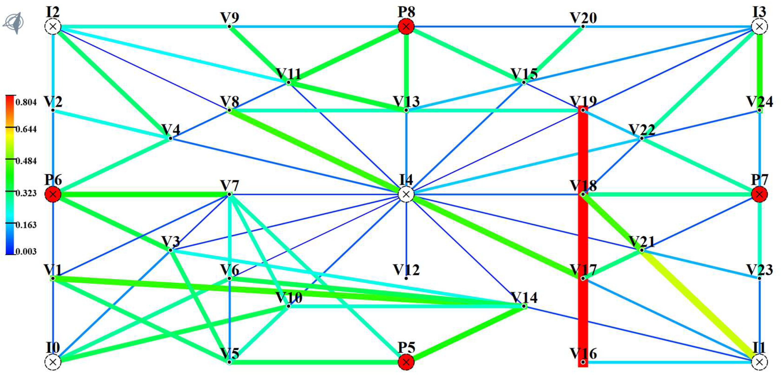
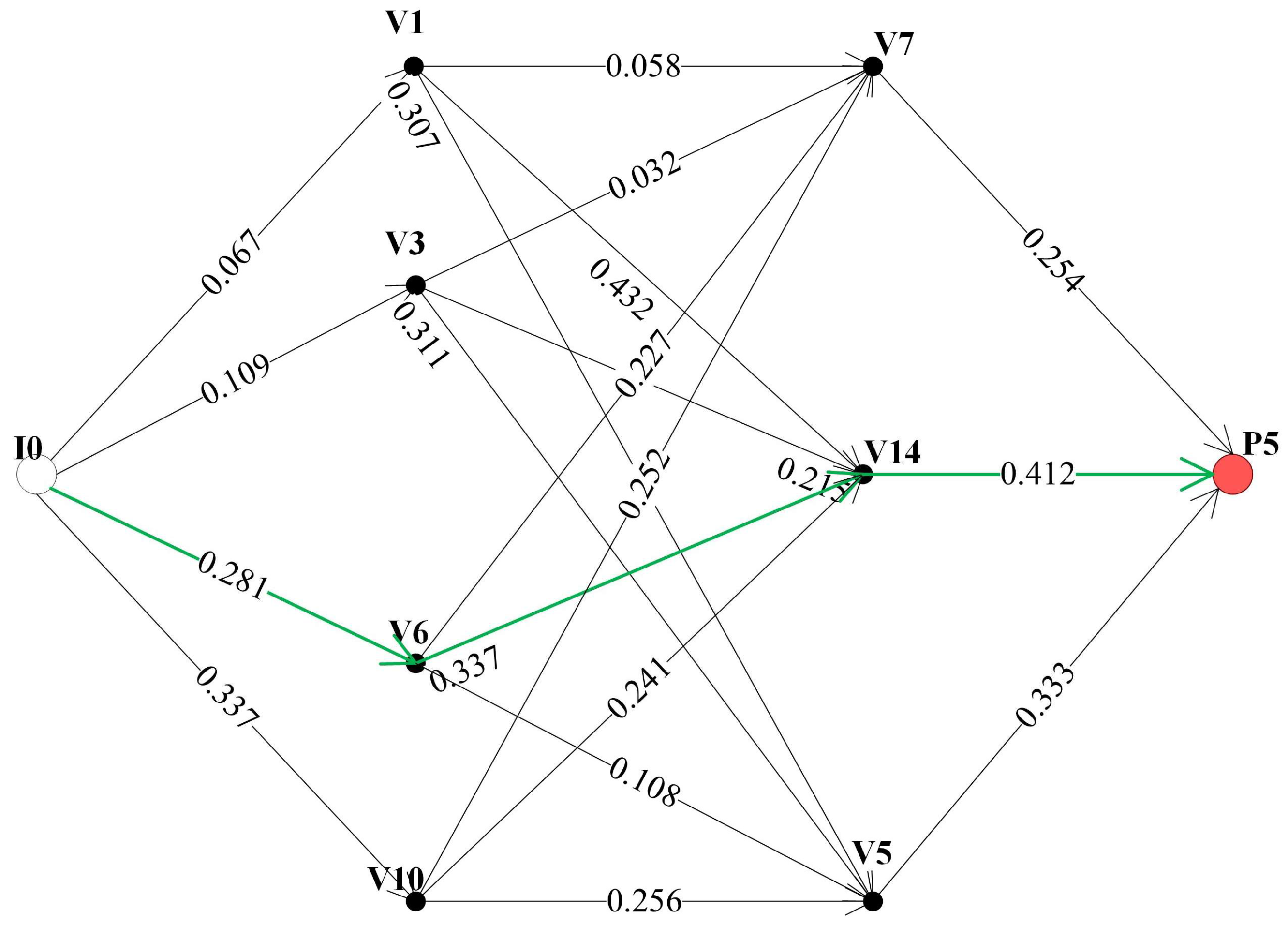
3.3. Connectivity Well Point Example Model Group

Based on the experiments with the two example models above, it can be anticipated that as the complexity of the model increases, the ACO algorithm will outperform the DFS algorithm. Therefore, a set of connectivity well point example models will be used to compare the computational efficiency of the ACO algorithm with that of the DFS algorithm. This model group analyzes a fixed pair of injection and production wells (in this experiment, wells 0 and 5).

To validate the efficiency of the ACO algorithm and explore the approximate range of complex models mentioned in this paper, a series of structurally similar but increasingly complex models will be used to trace advantageous paths. At this time, the hyperparameters of the ACO algorithm are as follows: num_ants = 150, num_iterations = 500, alpha = 1.0, beta = 2.0, evaporation_rate = 0.8, and q = 100. The specific model structures and time comparisons are shown in

Table 1. Time comparison of connectivity example models.

Number of Nodes	Number of Edges	Execution Time	Flow Path Data
22	84	DFS:0.0059s ACO:0.3776s	[0, 3, 8, 12, 16, 5] Split Factor:0.885198
32	169	DFS:0.2801s ACO:0.5052s	[0, 1, 11, 17, 24, 30, 5] Split Factor:0.533548
42	319	DFS:1.0464s ACO:0.6260s	[0, 9, 15, 22, 32, 5] Split Factor:0.857916
52	469	DFS:14.5559s ACO:1.9847s	[0, 4, 21, 27, 38, 50, 5] Split Factor:0.814488

below.

According to Table 1, when the number of nodes is 22 and the number of edges is 84, the DFS algorithm takes 0.0059 s, while the ACO algorithm takes 0.3776 s. The DFS algorithm is faster than the ACO algorithm. When the number of nodes is 32 and the number of edges is 169, the DFS algorithm takes 0.2801 s, and the ACO algorithm takes 0.5052 s. Again, the DFS algorithm is faster than the ACO algorithm. When the number of nodes is 42 and the number of edges is 319, the DFS algorithm takes 1.0464 s, while the ACO algorithm takes 0.6260 s. When the number of nodes is 52 and the number of edges is 469, the DFS algorithm takes 14.5559 s, while the ACO algorithm takes 1.9847 s.

Evaluations were performed on graphs of varying scales, characterized by node counts ranging from 22 to 52 and edge counts from 84 to 469, with computation times measured in seconds. For smaller-scale graphs, specifically those with 22 and 32 nodes, the DFS algorithm demonstrated superior computational efficiency compared to the ACO algorithm. In particular, for the graph comprising 22 nodes and 84 edges, the DFS algorithm’s computation time was 0.3716 s shorter than that of the ACO algorithm. Similarly, for the graph with 32 nodes and 169 edges, DFS exhibited a reduction in computation time by 0.2250 s. In contrast, for larger-scale graphs with 42 and 52 nodes, the ACO algorithm surpassed the DFS algorithm in computational performance. Specifically, for the graph with 42 nodes and 319 edges, the ACO algorithm reduced computation time by 0.4204 s, representing an efficiency improvement of 40.17%. For the graph with 52 nodes and 469 edges, the ACO algorithm outperformed DFS by 12.5711 s, yielding an efficiency improvement of 86.37%.

Overall, Table 1 data indicate that the ACO algorithm is superior to the DFS algorithm in terms of computational efficiency and stability when handling complex well-point models. It is also possible to confirm the approximate range of complex well point models, with the number of nodes ranging from 32 to 42 and the number of edges from 169 to 319 being classified as the complex well point models referred to in this paper.

4. Conclusions

This paper presents an exploration of the foundational principles for identifying optimal pathways within unstructured reservoir systems. It encompasses a detailed examination of pertinent computational formulas and the application principles of the ACO algorithm. The study offers a foundational methodology for addressing the challenge of advantageous path tracking through the utilization of the ACO algorithm. Furthermore, empirical investigations employing two real-world reservoir well point models, alongside a series of structurally analogous models, substantiate the efficacy of the ACO algorithm in resolving this issue. The experiments were conducted on a system equipped with an AMD Ryzen 9 7845HX processor with Radeon Graphics (3.00 GHz), 16 GB of RAM (15.2 GB available), and a 64-bit operating system running on an x64-based processor. The equipment was sourced from ASUS, based in Taipei, Taiwan. The findings substantiate that the ACO algorithm outperforms the conventional DFS algorithm in managing intricate well-point models.

In the experimental section of this paper, two reservoir numerical simulation models—one large and one small—are employed to validate and illustrate the feasibility and specific process of the ACO algorithm in advantageous path tracking. Additionally, to quantitatively assess the computational speed advantages of the ACO algorithm in large reservoir models, a series of simulated reservoir models were utilized for advantageous path tracking. The parameters of the ACO algorithm in the experiment were set to fixed values. The findings, derived from the final experimental results, are summarized in the following.

With increasing graph complexity, the ACO algorithm exhibited enhanced computational efficiency relative to the DFS algorithm, thereby underscoring its superiority in identifying optimal paths within large-scale reservoir models characterized by intricate geological structures.

This advancement addresses the instability and slow computation challenges associated with traditional methods when applied to complex, large-scale geological models.

Future research will primarily concentrate on optimizing the balance between computational speed and accuracy of the ACO algorithm in small-scale reservoirs, alongside the development of dynamic adjustment strategies for the algorithm. In the context of large-scale reservoirs, the computational efficiency of the ACO algorithm significantly exceeds that of the traditional DFS algorithm, with performance improvements becoming increasingly evident as complexity escalates. Nevertheless, due to the diverse connectivity complexities inherent in different reservoir models, employing a uniform set of ACO algorithm parameters may lead to suboptimal computational speed and inefficient allocation of computational resources. Consequently, future investigations will focus on analyzing the disparities among various reservoir models and implementing dynamic ACO algorithm parameters to enhance computational efficiency.

References

1. Liu, Y.; Rao, X.; Zhao, H.; Zhan, W.; Xu, Y.; Liu, Y. Generalized finite difference method based meshless analysis for coupled two-phase porous flow and geomechanics. Eng. Anal. Bound. Elem. 2023, 146, 184–203. [Google Scholar] [CrossRef]
2. Gilman, J.R. An efficient finite-difference method for simulating phase segregation in the matrix blocks in double-porosity reservoirs. SPE Reserv. Eng. 1986, 1, 403–413. [Google Scholar] [CrossRef]
3. Zhou, Y.; Xu, Y.; Rao, X.; Hu, Y.; Liu, D.; Zhao, H. Artificial neural network-(ANN-) based proxy model for fast performances’ forecast and inverse schedule design of steam-flooding reservoirs. Math. Probl. Eng. 2021, 2021, 5527259. [Google Scholar] [CrossRef]
4. Karimi-Fard, M.; Firoozabadi, A. Numerical simulation of water injection in 2D fractured media using discrete-fracture model. In Proceedings of the SPE Annual Technical Conference and Exhibition, New Orleans, LA, USA, 30 September–3 October 2001; Paper SPE-71615. SPE: Richardson, TX, USA. [Google Scholar]
5. Rao, X.; Xin, L.; He, Y.; Fang, X.; Gong, R.; Wang, F.; Dai, W. Numerical simulation of two-phase heat and mass transfer in fractured reservoirs based on projection-based embedded discrete fracture model (pEDFM). J. Pet. Sci. Eng. 2022, 208, 109323. [Google Scholar] [CrossRef]
6. Felippa, C.A. Introduction to Finite Element Methods; University of Colorado: Denver, CO, USA, 2004; p. 885. [Google Scholar]
7. Gingold, R.A.; Monaghan, J.J. Smoothed particle hydrodynamics: Theory and application to non-spherical stars. Mon. Not. R. Astron. Soc. 1977, 181, 375–389. [Google Scholar] [CrossRef]
8. Chen, Z.; He, Z.; Zhang, Q. Community detection based on local topological information and its application in power grid. Neurocomputing 2015, 170, 384–392. [Google Scholar] [CrossRef]
9. Garver, L.L. Transmission network estimation using linear programming. IEEE Trans. Power Appar. Syst. 1970, PAS-89, 1688–1697. [Google Scholar] [CrossRef]
10. Jacquemyn, C.; Jackson, M.D.; Hampson, G.J. Surface-based geological reservoir modelling using grid-free NURBS curves and surfaces. Math. Geosci. 2019, 51, 1–28. [Google Scholar] [CrossRef]
11. Chen, X.; Rao, X.; Xu, Y.; Liu, Y. An effective numerical simulation method for steam injection assisted in situ recovery of oil shale. Energies 2022, 15, 776. [Google Scholar] [CrossRef]
12. Zhao, H.; Zhan, W.; Chen, Z.; Rao, X. A novel connection element method for multiscale numerical simulation of two-phase flow in fractured reservoirs. SPE J. 2024, 29, 4950–4973. [Google Scholar] [CrossRef]
13. Coon, E.T.; Moulton, J.D.; Kikinzon, E.; Berndt, M.; Manzini, G.; Garimella, R.; Painter, S.L. Coupling surface flow and subsurface flow in complex soil structures using mimetic finite differences. Adv. Water Resour. 2020, 144, 103701. [Google Scholar] [CrossRef]
14. Zhou, C. A parallel adaptive finite element algorithm for numerical simulation of flows. Chin. J. Comput. Phys. 2006, 23, 412. [Google Scholar]
15. Zhao, H.; Xu, L.; Guo, Z.; Zhang, Q.; Liu, W.; Kang, X. Flow-path tracking strategy in a data-driven interwell numerical simulation model for waterflooding history matching and performance prediction with infill wells. SPE J. 2020, 25, 1007–1025. [Google Scholar] [CrossRef]
16. Zhou, H.; Zhang, Y.; Liang, X.; Zhang, J.; Xu, Y.; Liu, J. Liquid production splitting of multi-layer mining considering multiple factors. Pet. Reserv. Eval. Dev. 2022, 12, 945–950. [Google Scholar]
17. Issa, R.I. Solution of the implicitly discretised fluid flow equations by operator-splitting. J. Comput. Phys. 1986, 62, 40–65. [Google Scholar] [CrossRef]
18. Zhao, H.; Rao, X.; Liu, D.; Xu, Y.; Zhan, W.; Peng, X. A flownet-based method for history matching and production prediction of shale or tight reservoirs with fracturing treatment. SPE J. 2022, 27, 2793–2819. [Google Scholar] [CrossRef]
19. Kasahara, T.; Wondzell, S.M. Geomorphic controls on hyporheic exchange flow in mountain streams. Water Resour. Res. 2003, 39, SBH 3-1–SBH 3-14. [Google Scholar] [CrossRef]
20. Goldberg, A.V.; Harrelson, C. Computing the shortest path: A search meets graph theory. In Proceedings of the ACM-SIAM Symposium on Discrete Algorithms (SODA), Vancouver, BC, Canada, 23–25 January 2005; Volume 5, pp. 156–165. [Google Scholar]
21. Tarjan, R. Depth-first search and linear graph algorithms. SIAM J. Comput. 1972, 1, 146–160. [Google Scholar] [CrossRef]
22. Beamer, S.; Asanović, K.; Patterson, D. Direction-optimizing breadth-first search. Sci. Program. 2013, 21, 137–148. [Google Scholar] [CrossRef]
23. Pathak, M.J.; Patel, R.L.; Rami, S.P. Comparative analysis of search algorithms. Int. J. Comput. Appl. 2018, 179, 40–43. [Google Scholar]
24. Shi, L. Research on path planning method based on graph search algorithm. Highlights Sci. Eng. Technol. 2024, 97, 267–274. [Google Scholar] [CrossRef]
25. Mavrovouniotis, M.; Li, C.; Yang, S. A survey of swarm intelligence for dynamic optimization: Algorithms and applications. Swarm Evol. Comput. 2017, 33, 1–17. [Google Scholar] [CrossRef]
26. Prity, F.S.; Uddin, K.A.; Nath, N. Exploring swarm intelligence optimization techniques for task scheduling in cloud computing: Algorithms, performance analysis, and future prospects. Iran J. Comput. Sci. 2024, 7, 337–358. [Google Scholar] [CrossRef]
27. Ouyang, J.; Yan, G.R. A multi-group ant colony system algorithm for TSP. In Proceedings of the 2004 International Conference on Machine Learning and Cybernetics (IEEE Cat. No. 04EX826), Shanghai, China, 26–29 August 2004; Volume 1, pp. 117–121. [Google Scholar]
28. Che, G.; Liu, L.; Yu, Z. An improved ant colony optimization algorithm based on particle swarm optimization algorithm for path planning of autonomous underwater vehicle. J. Ambient. Intell. Hum. Comput. 2020, 11, 3349–3354. [Google Scholar] [CrossRef]
29. Fleischer, R.; Trippen, G. Experimental studies of graph traversal algorithms. In Proceedings of the International Workshop on Experimental and Efficient Algorithms, Ascona, Switzerland, 26–28 May 2003; Springer: Berlin/Heidelberg, Germany; pp. 120–133. [Google Scholar]
30. Chen, X.; Yu, L.; Wang, T.; Liu, A.; Wu, X.; Zhang, B.; Sun, Z. Artificial intelligence-empowered path selection: A survey of ant colony optimization for static and mobile sensor networks. IEEE Access 2020, 8, 71497–71511. [Google Scholar] [CrossRef]
31. Mohan, B.C.; Baskaran, R. A survey: Ant colony optimization based recent research and implementation on several engineering domains. Expert Syst. Appl. 2012, 39, 4618–4627. [Google Scholar] [CrossRef]
32. Chen, Y.; Bai, G.; Zhan, Y.; Hu, X.; Liu, J. Path planning and obstacle avoiding of the USV based on improved ACO-APF hybrid algorithm with adaptive early-warning. IEEE Access 2021, 9, 40728–40742. [Google Scholar] [CrossRef]
33. Wu, J.; Chen, B.; Zhang, K.; Zhou, J.; Miao, L. Ant pheromone route guidance strategy in intelligent transportation systems. Phys. A 2018, 503, 591–603. [Google Scholar] [CrossRef]
34. Gang-Li, Q.; Jia-Ben, Y. An improved ant colony algorithm based on adaptively adjusting pheromone. Inf. Control 2002, 31, 198–201. [Google Scholar]
35. Gutjahr, W.J.; Rauner, M.S. An ACO algorithm for a dynamic regional nurse-scheduling problem in Austria. Comput. Oper. Res. 2007, 34, 642–666. [Google Scholar] [CrossRef]
36. Luan, J.; Yao, Z.; Zhao, F.; Song, X. A novel method to solve supplier selection problem: Hybrid algorithm of genetic algorithm and ant colony optimization. Math. Comput. Simul. 2019, 156, 294–309. [Google Scholar] [CrossRef]
37. Zhan, W.; Zhao, H.; Rao, X.; Liu, Y. Generalized finite difference method-based numerical modeling of oil–water two-phase flow in anisotropic porous media. Phys. Fluids 2023, 35, 103317. [Google Scholar] [CrossRef]
Figure 1. Inter-well flow connectivity in an equilateral triangle model.
Processes 13 00404 g001
Figure 2. Splitting coefficients in the equilateral triangle model.
Processes 13 00404 g002
Figure 3. Path {1, 4, 6, 2}.
Processes 13 00404 g003
Figure 4. Flowchart of the Ant Colony Optimization Algorithm.
Processes 13 00404 g004
Figure 5. Connectivity diagram of example Model 1.
Processes 13 00404 g005
Figure 6. Connectivity path from I0 to P5 and its unit-splitting coefficients.
Processes 13 00404 g006
Figure 7. The advantageous path results for example model 1.
Processes 13 00404 g007
Figure 8. Connectivity diagram of the complex model with two well points.
Processes 13 00404 g008