Development of Digital Twins for Continuous Processes: Concept Description of Virtual Mass Balance Based on the Tennessee Eastman Process

Abstract

In this work, the authors describe a concept called Virtual Mass Balance and its applicability to oil and gas fields. This study relies on data modelling and data engineering to enrich operational data and achieve digitized Material Balance Tables for monitoring and benchmarking purposes. A data-driven set of stream properties allow for the calculation of newly proposed soft sensors, which are subsequently used for predictive functionalities. The implementation of this concept has proven popular in an industry set of tools, AVEVA PI. The concept could be classified as an Enriched Digital Twin. Incorporating the DEXPI Process model and deploying proposed soft sensors could, on the one hand, combine both asset and operational characteristics. On the other hand, its simplicity and moderate level of detail can be much easier to implement and would show flexible applicability at various corporate levels. The application of the Tennessee Eastman Process proves its flexibility. The presented soft sensors exhibit good monitoring capabilities and, furthermore, allow for the application of data-driven artificial intelligence methods without a reduction in model clarity for operational staff.

1. Introduction

Digital transformation, understood as Industry 4.0 in the petroleum and petrochemical sector, is a fact. Consequently, terms such as Digital Twin (DT), soft sensor, artificial intelligence (AI) and machine learning (ML) have been introduced into the vocabulary of engineers previously focused on conducting production processes. There are a number of publications which explore the systematic classification of data-driven methods, their pros and cons [1], and their applicability to the oil and gas industry and organization [2,3,4,5], together with Industry 4.0-specific technologies and sustainability impacts [6,7,8]. Many authors have not only identified the possibilities and prospects of these technologies for industry, but have also described implementation examples, especially for the upstream sector of the oil and gas industry—applications for large volumes of subsurface data analysis, drilling equipment decision-making support and predictive maintenance have been described [1,4,9]—as well as for the downstream sector, including yield predictions for thermal cracking [10], FCC [11], and steam cracking [12], and general cases applicable to the process industry [13] where MSE values might range from 10⁻³ [10] to 0.8 [11]. Furthermore, optimization tasks were presented which indicate promising benefits, even 21.21 × 10⁶ USD/y [14].

Section 2 of this paper is focused on an analysis of the literature related to Digital Twins. The authors discuss aspects related to defining the DT concept and their possible industrial implementations as a whole, as well as in an individual organizational context. Section 3 includes a brief description of the Tennessee Eastman Process, an example from the literature, popular in scientific publications, created by Downs and Vogel in 1993 [15], based on which the newly presented concept of Virtual Mass Balance (VMB) is described. Section 4 includes a generic presentation of the solution, along with considerations regarding the data model and the development of three layers. The multidimensionality of VMB is presented, showing the possibility of coupling DESIGN, REAL, and MODEL layers for monitoring applications and the creation of data-driven predictions. Furthermore, the authors performed the study according to the archetypes indicated in the work of van der Valk, Haße, Moller, and Otto [16], which can be classified as and named Digital Twins. The aim of Section 5 is to discuss possible use cases for VMB deployment and to identify challenges for further development.

The presented concept suits the approach described by Aivaliotis, Georgoulias, Arkouli, and Makris [17], where the first phase involves recreating the structural process model, followed by elaborating on the virtual sensors, enabling monitoring and reflection of actual data during simulation. The third phase involves defining operational parameters collected in real time, allowing for model updates.

The proposed form of soft sensors comprises a set of the directional coefficients created based on historical process data and the calculated mass balance of the unit. To the best of the authors’ knowledge, such an approach has not been presented in the literature so far. The concepts of the proposed soft sensors, the main assumptions and possible applications of VMB are described in this paper. The concept does not have any literature references yet, but industrial tests indicate promising results.

2. Issues Related to Digital Twins

2.1. Digital Twins in Science

The concept of a “Digital Twin” is currently very popular in many fields of science, as confirmed by the analysis conducted by Tao, Xiao, Qi, and Cheng [18]. As a rule, a synchronized, virtual reflection of a physical object is defined as a twin, as stated by Jasiulewicz-Kaczmarek [8], among others. Digital Twins are present in almost every area of life [18], despite being considered a relatively new research branch, and from a scientific point of view, the DT concept may constitute a wide area for potential development. Despite the dynamically growing number of publications, there has not yet been an unequivocal definition of a twin specifying the method of implementation, nor a study of the tools dedicated to this class of solution. Van der Valk, Hunker, Rabe, and Otto have tried to describe a taxonomy related to twins [19], where they identified seven dimensions characterizing simulation models using 14 possible attributes and then proposed an analogous taxonomy for twins, based on which five DT archetypes were identified [16]; each subsequent one includes a predecessor by expanding its scope. However, the authors emphasized that the proposal is subjective and other scientists may define this field differently, an example of which can be seen in the work of Harper, Malakuti, and Ganz [20].

2.2. Digital Twins in Industry

Looking at twins from an industry perspective and following market trends in the chemical and manufacturing fields, two main trends can be distinguished. The first is the “Asset Digital Twin” [21,22], the main role of which is to collect information from the full life cycle of the asset from various systems and contextualize the complete set of available data within a given unit or device, often combined with operational indications in close-to-real time. This type of solution is often related to data interoperability; thus, its main consideration is the development and maintenance of the data model and its exposure to business processes. Contextualization applies to both engineering data from the design phase (schemes, data sheets, 3D models, technical documentation) [23,24,25,26] and data from various domain systems available in the organization, e.g., records from operator inspections and planning and scheduling data (regarding the operation status of devices and units, quality information, data from sensors and current limitations). Data regarding the final stage of the particular device lifetime are also used [27]. All information packed in the context of a specific asset allows its current and historical state to be reflected and is present in almost every domain. However, it does not reflect simulation capabilities (prediction or optimization ones). Twins of this type do not have a single standard, but it is possible to identify standards or methodologies such as ISO 23247 [28], CFIHOS [29], ISO 15926 [30], ISO 14306 [31], IMF [26], DEXPI [25], and AAS, as well as ISA88 [32], ISA95 [33] or IEC PAS 63088 [34], that support the construction of such solutions. The examples of “Asset Digital Twin” applications are presented below:

• Mapping the physical layout of assets, e.g., for training purposes, or as a basis for a metaverse;
• Operational management by providing fast access to information from many sources regarding a given asset (including information about related procedures and documentation);
• Monitoring the progress of investment projects and the completeness of information;
• Remote engineering support for people working in a facility;
• Identification of threats (both with respect to process and personnel);
• Easier implementation of predictive maintenance solutions.

The next interpretation is the “Process Digital Twin”, which, unlike the one presented earlier, focuses primarily on simulation aspects. This type of solution can be a coherent extension of the “Asset Digital Twin” or it can constitute an independent instance. According to the thesis presented in van der Valk’s work [19], taxonomies of this type of twin can be determined based on seven dimensions:

(I)

Time step [continuous/discrete];

(II)

Probability [deterministic model/stochastic model];

(III)

Model nature [static/dynamic];

(IV)

Use of the process model [for simulation purposes/not for simulation purposes];

(V)

Model scope [single element/system of interrelated elements];

(VI)

Verification and validation [verified and validated model/unverified and invalidated model];

(VII)

Time horizon [definite/indefinite].

Describing the nature of the model in these dimensions should quite well determine the possible technologies and solutions that could suit the twin. Dimension III may be expanded and clarified, in which rigorous models can be assigned to deterministic models (according to the authors, they do not take into account any properties in terms of probability), while stochastic ones include solutions based on data. However, in industrial practice, it is impossible to meet the condition in which the data input for deterministic models is not subjected to processing and preparation for simulation purposes (including the use of statistical analysis). Otherwise, asynchrony in access to various types of data would cause numerous inconsistencies, and thus, the results would not be reliable. This is a typical phenomenon in the decision-making process: “garbage in, garbage out” (GIGO).

For this type of twin, the range of solutions and applications is wide, strongly dependent on the purpose for which the model was developed. The exemplary applications of a properly developed process twin include the following:

• Creating predictions of yields and the operation of particular systems;
• Determination of physicochemical parameters or process variables in places where there is no measuring equipment installed;
• Support for engineers in conducting the process by suggesting optimal solutions;
• Using the model as an operator training station (OTS).

2.3. Digital Twins in Organizations

Implementing and maintaining any of the previously discussed Digital Twins is a significant challenge for organizations. To carry out these types of tasks, a number of conditions are necessary for the implementation of the DT project, including the availability of appropriate IT architecture and applications, as well as software tools. The key is, above all, available digitized data resources, which, even within one organization, may differ between assets or units (e.g., due to age or other conditions). This contributes to the difficulties in scaling the solution, limiting the scope of its impact.

To consider scaling aspects, especially in terms of process DTs, Guerra and Roux [35] presented the multidimensional relationship of the hierarchical organizational structure and its impact on the complexity and accuracy of models describing individual process units or equipment in a diagram (Figure 1). Digital Twins with possibly the biggest profits might be useless from an operational point of view due to their simplicity. The required implementation and computational contributions are also taken into account. There is a visible discrepancy between the operational level and scheduling. At the lowest operational layer, where the time scale is in seconds, deterministic models seem to be the most useful; they are tedious to develop and maintain but are based on physicochemical laws governing unit processes. Areas above production—scheduling and planning—work with data on an hourly/daily basis or for longer periods such as decades/weeks/months. This perspective allows for simplifying the complexity and constructing stochastic, empirical models. Areas at this level of the hierarchy influence the definition of global goals, which translates most into the benefits of twin models implemented at this level of the organizational hierarchy. The focus of these models is on maximizing the benefits of the company, not the operation of the installation itself. Tsay and Baldea [36] discuss in their article how data can be a bridge connecting different needs at different levels (referring to different scales of time and distance). The question remains, how do we avoid building many models, or at least how do we maintain synergies between them? The hypothesis defined by the authors indicates that it is historical operational data and their analysis that may allow for the improvement of empirical models and, at the same time, for the construction of data-driven solutions that may be useful in scheduling or planning (decisions made are based on relatively wide time scales and large scope in the organization, e.g., several process units in the production line).

3. Tennessee Eastman Process

In the 1990s, for the needs of the academic community, Downs and Vogel presented a process based on an actually operating installation belonging to the Eastman Chemical Company [17]. The authors of the model made appropriate modifications to both chemical compounds and kinetics and process variables in order to conceal intellectual property; nevertheless, the presented description and data reflect a realistic process and problems that the chemical industry still faces and identifies with. Since then, many scientific contributions referring to the presented model have been published. The scope of these works might be divided by the following subjects: process control [37,38,39], real-time optimization [40,41,42,43,44,45], process monitoring and fault detection [46,47,48,49,50], process modelling and forecasting [11,51,52,53,54,55,56], data quality [57] and datasets [55,58,59].

The process shows a node that includes a reactor, a post-reaction stream cooler, a liquid–steam separator and a packed separation column heated by steam. Chemistry is based on eight compounds (A, B, C, D, E, F, G, H), of which A, C, D and E are substrates, G and H are main products, F is a by-product and B is inert. Four streams (#1—A; #2—D; #3—E; #4—C) constitute the input to the process; A (#1), D (#2) and E (#3) as well as the top stream of the separator (#5) and post-reaction recycler (#8) constitute the input to the reactor system.

The stream downstream of the reactor is cooled. Reaction products condensed in the separator are directed to the stripper (#10), and the gaseous phase is partly purged (#9—PURGE) and partly recycled (#8). The stripper receives two streams: the C feed in the gas phase (#4) and the condensate from the separator (#10). The product stream as the liquid phase (#11—product) is a mixture of mainly G and H compounds routed outside battery limits. Stream from the top is routed to the reactor. The process is controlled by 41 variables (XMEAS). Variables 1–22 are indications of temperature, pressure, flow or level and power, while 23–41 are quality measurements of online analyses. Data contained in Vogel’s article will be treated as engineering data for the purposes of the example discussed.

4. Virtual Mass Balance Concept

The concept of Virtual Mass Balance (VMB) is presented in Figure 2, defined as a data model of a particular process unit with a dedicated end user interface, which represents three layers of related process states: DESIGN, REAL and MODEL. Each of them reflects a set of dedicated tables: Stream, Balance and Virtual Coefficients. The shape of particular tables between layers is consistent, but the source and/or transformation of data might differ. The basis for Stream Tables is Heat and Material Balance and, in fact, might be taken from engineering documentation. Nevertheless, operational data require a data engineering approach in order to reveal the complete set for REAL data and might differ from case to case. Balance and Coefficient Tables are the main subject of this concept. The development of the VMB begins with the DESIGN layer, proceeding to REAL and ending at the MODEL part. The possibilities and usability of the last layer are very flexible; thus, its development and customization might be different from case to case.

The concept involves real-time mapping of streams reflected in the process Material Balance of a given process unit, allowing for the calculation of coefficients proposed by the authors on a near-real-time basis, which act as soft sensors for monitoring purposes and—at the same time—are hyper-parameters of the unit’s mathematical model.

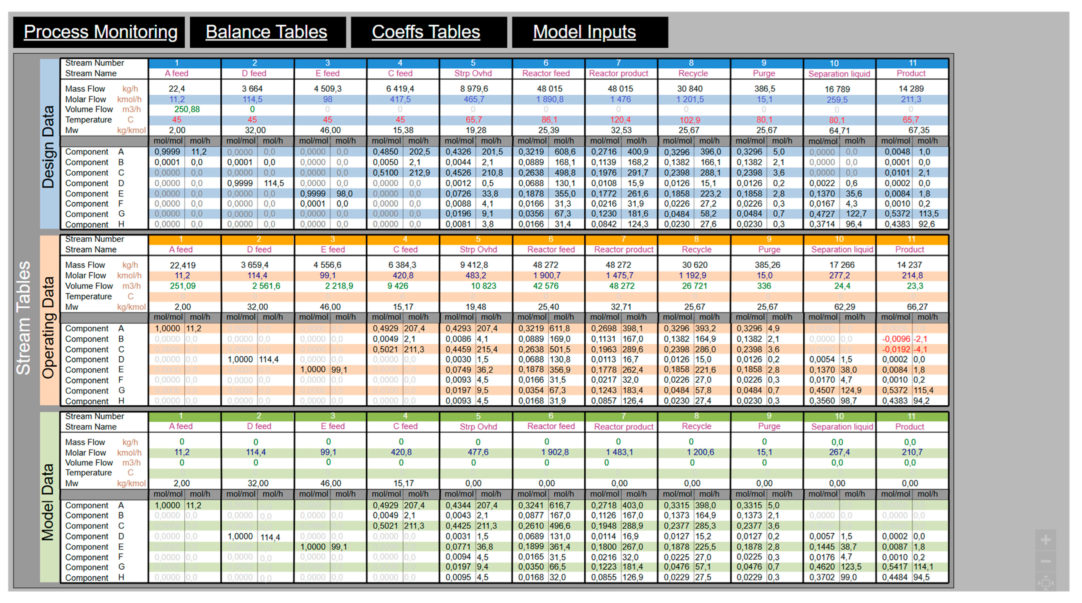
4.1. The VMB Data Model

A moderate level of detail and complexity, together with the principal idea of the VMB, result in a range of information from Process Flow Diagrams that is sufficient to develop and reflect a particular process. The main advantage of this assumption is that PFD’s complexity is not problematic (especially in comparison to P&ID’s) for people not involved in the chemical process on a daily basis (allocated within level 3 and 4 in the organizational pyramid—Figure 1). On the other hand, this engineering documentation reflects the topology of the main assets across the process unit and, together with the Process Heat and Material Balance, provides information about the crucial technological state of the process. The abovementioned aspects have been covered by the DEXPI Process standard and data model which is considered as a basis for VMB.

The DEXPI Process data model [23,24,25] was created for information management of engineering documentation and integration of existing standards. It allows for transfer of information covered by PFD in a manner readable by machines. The data model is adopted and slightly extended, providing adjustments for the purpose of VMB. Such an approach provides a simple reference to existing semantics and standards, used across industrial enterprise architectures [23]. Figure 3 shown below presents how process topology between particular Process Steps is modelled and where streams are situated.

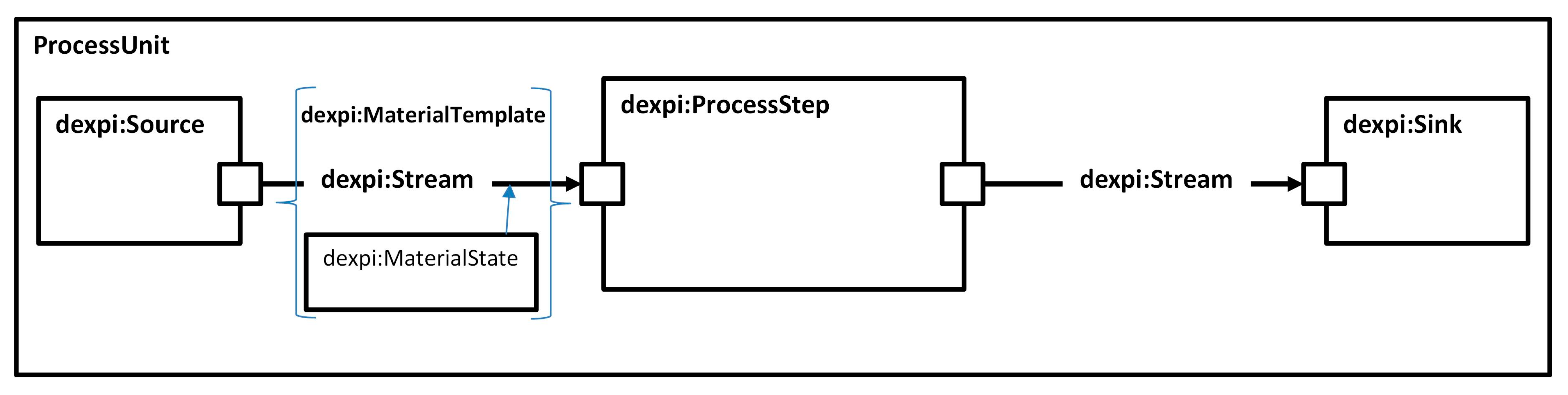
4.2. VMB Tables

The concept assumes that each layer is represented by a set of tables, which are consistent and mirrored across all layers in terms of scope but differ in terms of the source of data and values. The following tables are represented:

(a)

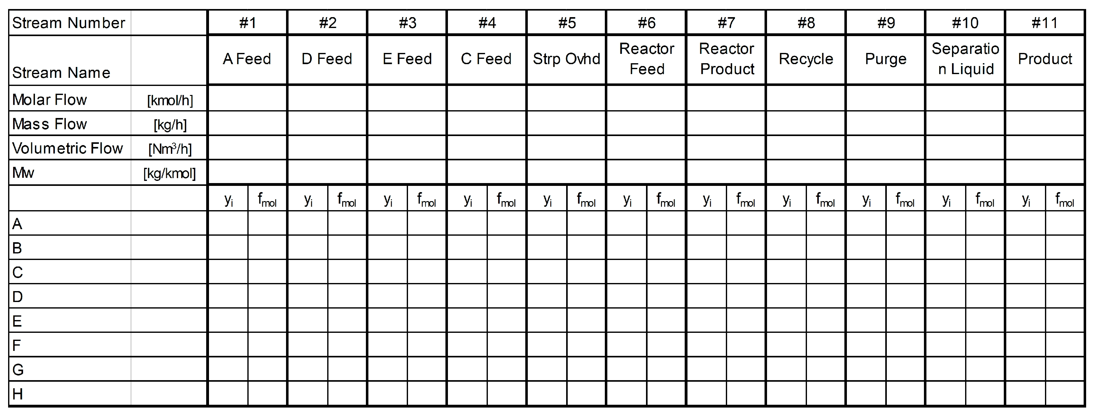
Stream Table

This is a well-known set of all streams included in PFD, which connect the main Process Steps. The shape of the table, depending on the process unit and available data, might vary from case to case. Thus, the data model should be customizable in terms of components and properties presented for each unit. The DEXPI Process data model considers these concerns and naturally fits the Virtual Mass Balance Stream Table purpose as well. Thus, it has been adopted and treated as the basis for further development of the VMB data model. Depending on the architecture of particular implementation, the proposed data model might be changed and adjusted accordingly.

Figure 4 presents the shape of the Stream Table specified for the Tennessee Eastman Process, including 11 streams indicated on the process flowsheet. Engineering data, which the authors assumed to be as in the Downs and Vogel publication [15] (for the purpose of this presentation), covered information about mass flow, molecular flow and mole fractions. In order to show other properties, some basic chemical transformations should be performed. For the DESIGN layer, the values in the table are static and are taken from engineering documentation (basically, PFDs, Material Balance or other available sources). In the case of the REAL layer, the table reflects operational data (typically from the process historian, laboratory results from the LIMS system, etc.); the architecture of the solution might be different and depends on the organizational landscape. The MODEL layer’s table generally is a final solution of calculations performed based on input data. It represents the prediction of all stream properties.

(b)

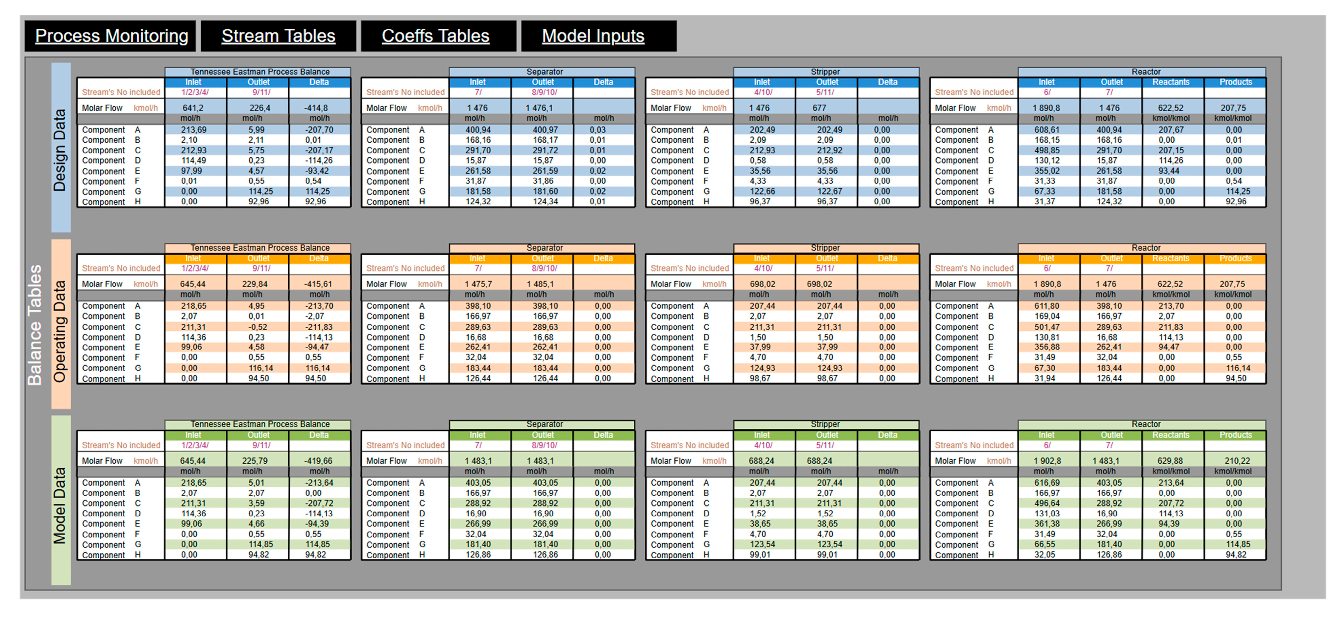
Balance Tables

Tables are dedicated to visualizing the overall process balance together with a set of subprocesses included in the unit. The information it provides is useful for tracking possible inconsistencies and quickly addressing them during process monitoring tasks. Figure 5 presents the proposed data model for Balance Tables. The main class could be divided into Balance Table_Unit, which is essentially applicable for the whole considered process unit. Another specialization of the BalanceTable is BalaceTable_ProcessStep, where BalanceTable_Separation and BalanceTable_ReactionChemicals might be distinguished. Both are associated with an adequate ProcessStep Class from the DEXPI Process model. The composition of specific columns is determined by the type of ProcessStep; nevertheless, all kinds of Balance Tables are assigned to a particular Layer and consist of InletColumn, OuteltColumn and Delta Column classes, which provide a set of flow values for each component included in VMB, treated as QualifiedPhysicalQuantity—MoleFlow or MassFlow. Values for particular components might be the subject of BalanceCalculation where the following equations might be applied:

• BalanceCalculation_Sum (1) is applicable for calculating the Inlet, Outlet, and direction values based on a particular ListOfIncludedStreams subclass.
• BalanceCalculation_Delta (2) is dependent from Inlet and Outlet streams of a particular BalanceTable.
• BalanceCalculation_Reacted (3) is calculated for ReactingChemicals Process Steps; the dependency on delta value is reflected.
• BalanceCalculation_Produced (4) is calculated based on delta value and associated with reactive systems.

For chemical reactions, Equation (6) should also be applied.

f_iSUM = Σ_xf_i where x ∈ {ListOfIncludedStreams}

(1)

delta_i = f_iOUTLET − f_iINLET

(2)

delta_i < 0: |delta_i| = f_iREACTED

(3)

delta_i > 0: delta_i = f_iPRODUCED

(4)

delta_i = 0 = f_iINERT

(5)

F_REACTED = F_PRODUCED = Σf_iPRODCUED

(6)

(c)

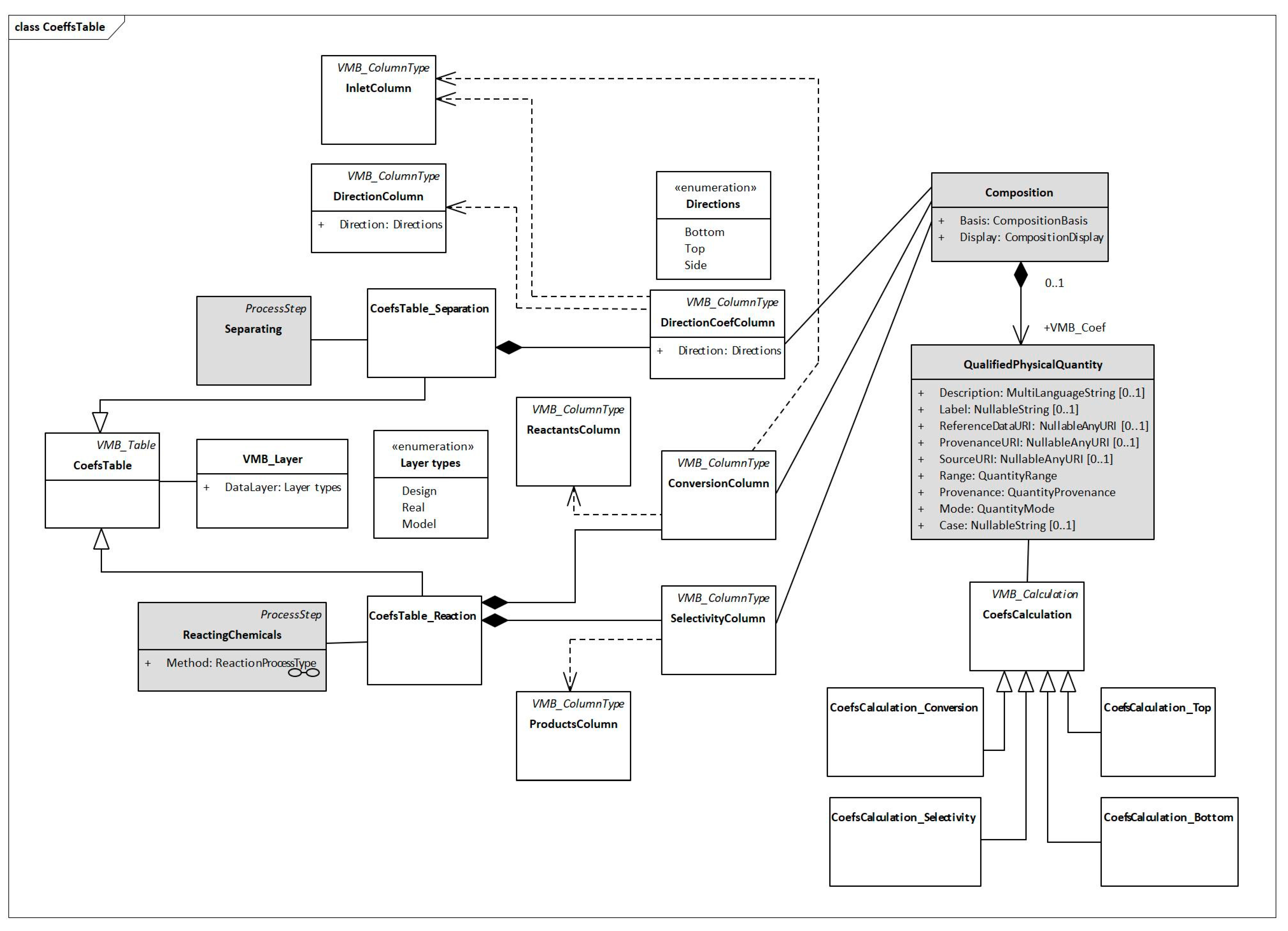
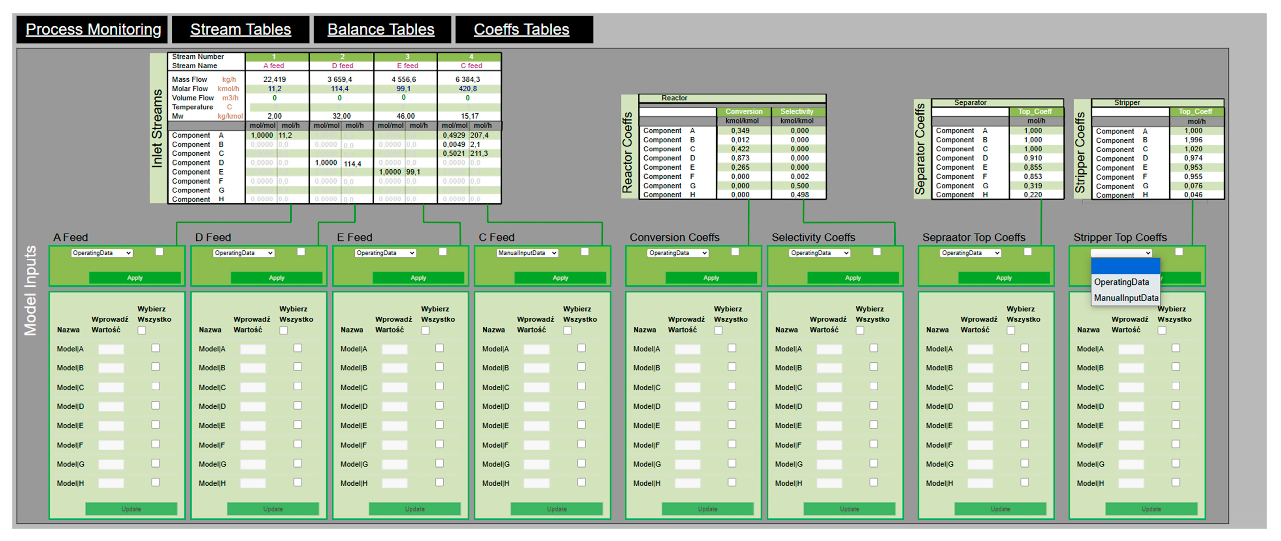
Virtual Coefficient Tables

The aim of these tables is to expose proposed soft sensors calculated based on values expressed in BalanceTables.

For Separating Process Step subclasses, where splitting of individual compounds takes place, determined variables—called direction coefficients—indicating what share of the i-th compound flows (f_i,d) towards direction (d) are from its total “INLET” pool (F_iINLET) (1). Directions reflect particulate MaterialPort outlets from the Separating Process Steps. It is, however, important that the following relations are maintained: Balance should be as per Equation (8); the coefficient ranges from 0 to 1 (9); and the sum of the shares of given coefficients for the i-th compound in all directions is 1 (10).

coef_d,i = f_i,d/F_iINLET

(7)

F_iINLET = F_iOUTLET

(8)

coef_d,i ∈ <0, 1>

(9)

Σ_dcoef_i = 1

(10)

In chemical reaction systems, the balance helps determine the number of substrates and the corresponding amount of reaction products. Based on the balance (1)–(10), conversion rates (coef_iCONV) (11) and selectivity (coef_iSEL) (12) for individual i-th compounds are determined.

coef_iCONV = |delta_i|/f_iINLET

(11)

coef_iSEL = f_iPRODUCED/F_REACTED

(12)

Σcoef_iSEL = 1

(13)

The logic described above is reflected in the data model presented in Figure 6. CoefsTable is assigned to the dedicated VMB_Layer. There are two possible subclasses:

CoefsTable_Separation is dedicated to the ProcessStep where separation occurs. For such operations, tables consist of the DirectionCoefColumn, presenting values of soft sensors for particular components which are classified as QualifiedPhysicalQuantity—VMB_Coef (possibly subclass of “Ratio” parameter). Direction coefficients are estimated with an appropriate CoefsCalculation subclass—CoefCalculation_Top or CoefCalculation_Bottom—based on Equation (7). A CoefsTable dedicated to the separation type of ProcessStep might optionally include InletColumn and DirectionColumn, which are the subject of BalanceTables and are the basis for coefficient calculations.

CoefsTable_Reaction is assigned to the ReactingChemicals ProcessStep and consists of the ConversionColumn and SelectivityColumn. These columns contain values of QualifiedPhysicalQuantity specified as VMB_Coefs and calculated accordingly: CoefsCalculation_Conversion based on Equation (11) and CoefsCalculation_Selectivity based on Equation (12). There is also an option to include ReactantsColumn and ProductsColumn, both from BalanceTable.

4.3. VMB Layers

Three interfering layers coupled with each other are distinguished by the presented concept. Despite each of them having the same components, their roles and functionalities are different:

(a)

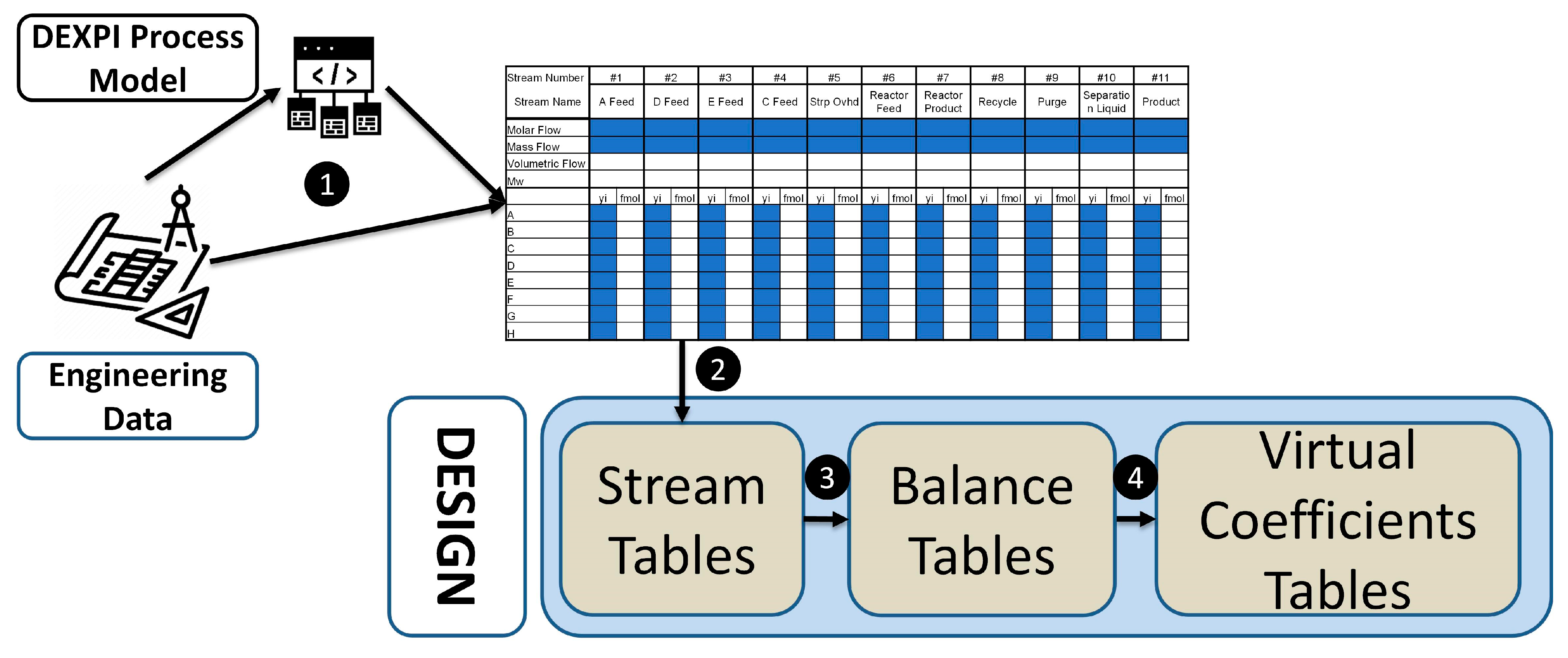
The DESIGN layer development flow is shown in Figure 7. The sources of data for this layer are engineering files, especially PFDs and Material Balance. Often, the Stream Table supplied by the contractor is limited to only a few properties, which might be hard to interpret or evaluate on first sight (Figure 7, point (1)). As previously described, documented values might be incorporated into the VMB data model seamlessly by the deployment of the DEXPI Process concept or even manually. In case of TEP, the engineer would only see the partially filled table. Simple chemical calculations and transformations allow for filling all required parts of the Stream Table (Figure 7, point (2)). These properties (especially mass or molar flow) are then used for the calculation of the Process Balance Table (Figure 7, point (3)). Virtual Coefficients are also shown in dedicated tables (Figure 7, point (4)). Steps 3 and 4 are generic based on data model configuration.

The described layer plays a mostly informative, benchmark role. The possible enrichment of the Stream Table might be useful during commissioning or Performance Test Runs, as it could give relevant background for process condition checks against design values. In some cases, the DESIGN data might be useful while making assumptions for calculation steps in other layers.

(b)

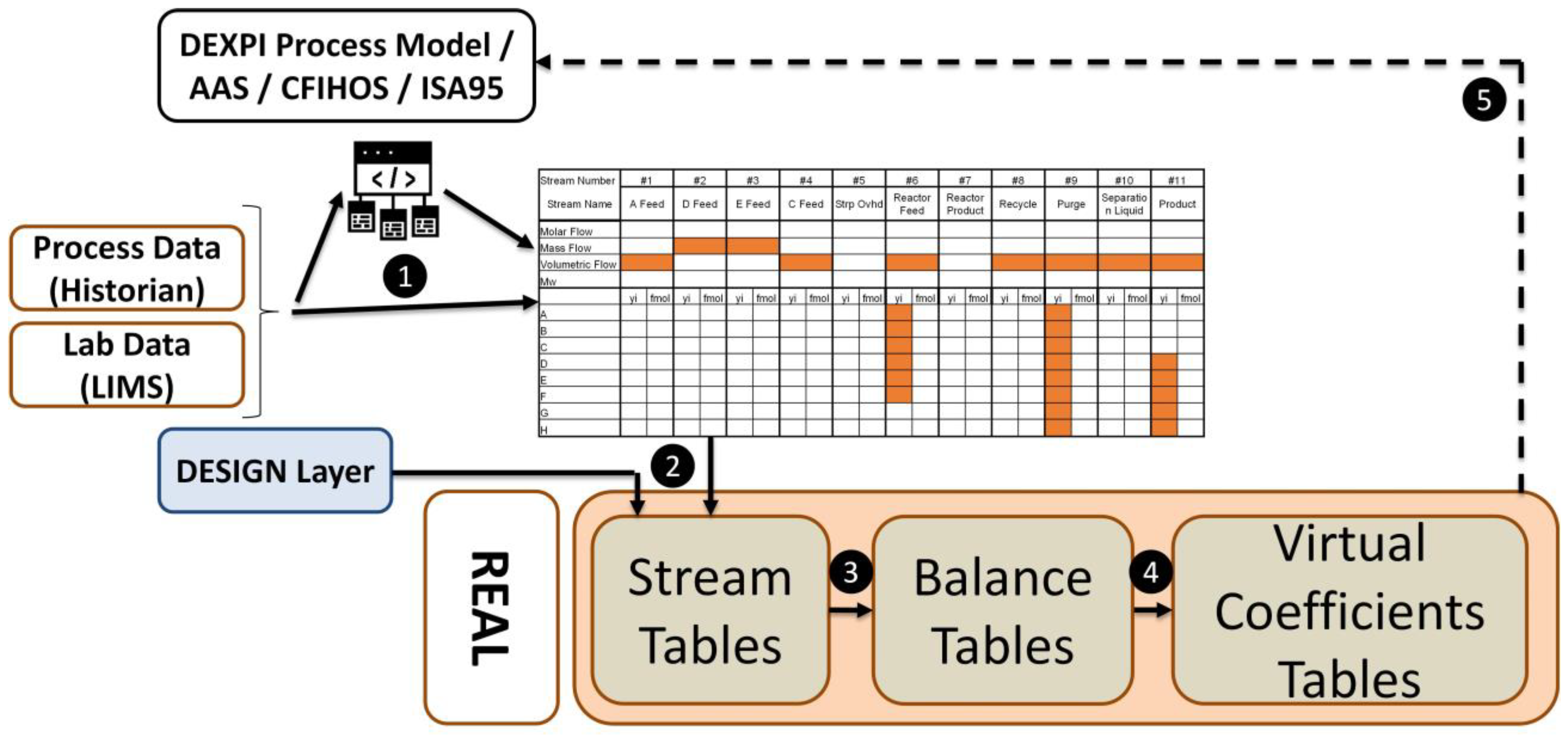
In the case of the REAL layer, the main difference is caused by the fact that, when comparing a nearly complete set of design values, the operational data are typically limited to those needed for process control and safety (stored as timeseries and available usually from the Historian database). Another important aspect is the limited availability of quality data, typicaly acquired from LIMS at a predefined schedule. Figure 8, point (1), shows possible data sources. Data might be acquired by a point-to-point connection or integrated with existing data models available within enterprises (adoption and extension of the DEXPI Process data model should ease that possibility). Independently from the data aquisition aspect, available data are sufficient to fill the Stream Table only partially. An essential feature of the VMB concept is to show off a complete set of stream properties in order to (among others) enhance operational monitoring. Figure 8, point (2), refers to the set of calculation steps performed on a predefined schedule to provide all relevant stream properties required by further steps. The number of steps and calculations is case-sensitive, and authors of the VMB concept assume that most of them are just mass balance-dependent (derived of “modelling” mixing or splitting parts, where the DEXPI Process data could also help). Besides simple arithmetic, some assumptions made by Subject Matter Experts are required to meet the main goal. The set points of process variables are useful as well. It seems important to include within the VMB data model the place where the number of steps and equations/assumptions with remarks could be included. Further steps, related to the calculation of Balance Tables and Coefficients (Figure 8, points (3) and (4)), are the same for the DESIGN layer. The dashed line mark in Figure 8 as point (5) is optional and related to the possible enrichment of the enterprise data model by VMB calculations.

The Exemplary TEP Process provides 41 operating variables that are measured and visible to operators. Stream flow units are mixed; some of them are given in volumetric flow, and others as mass flows, while quality measures are presented as molar fractions. This causes interpretation difficulties. Thus, the most important function of this layer is to provide completeness in the Stream Table and increase process conciousness and monitoring capabilities by tracking soft sensors’ values.

(c)

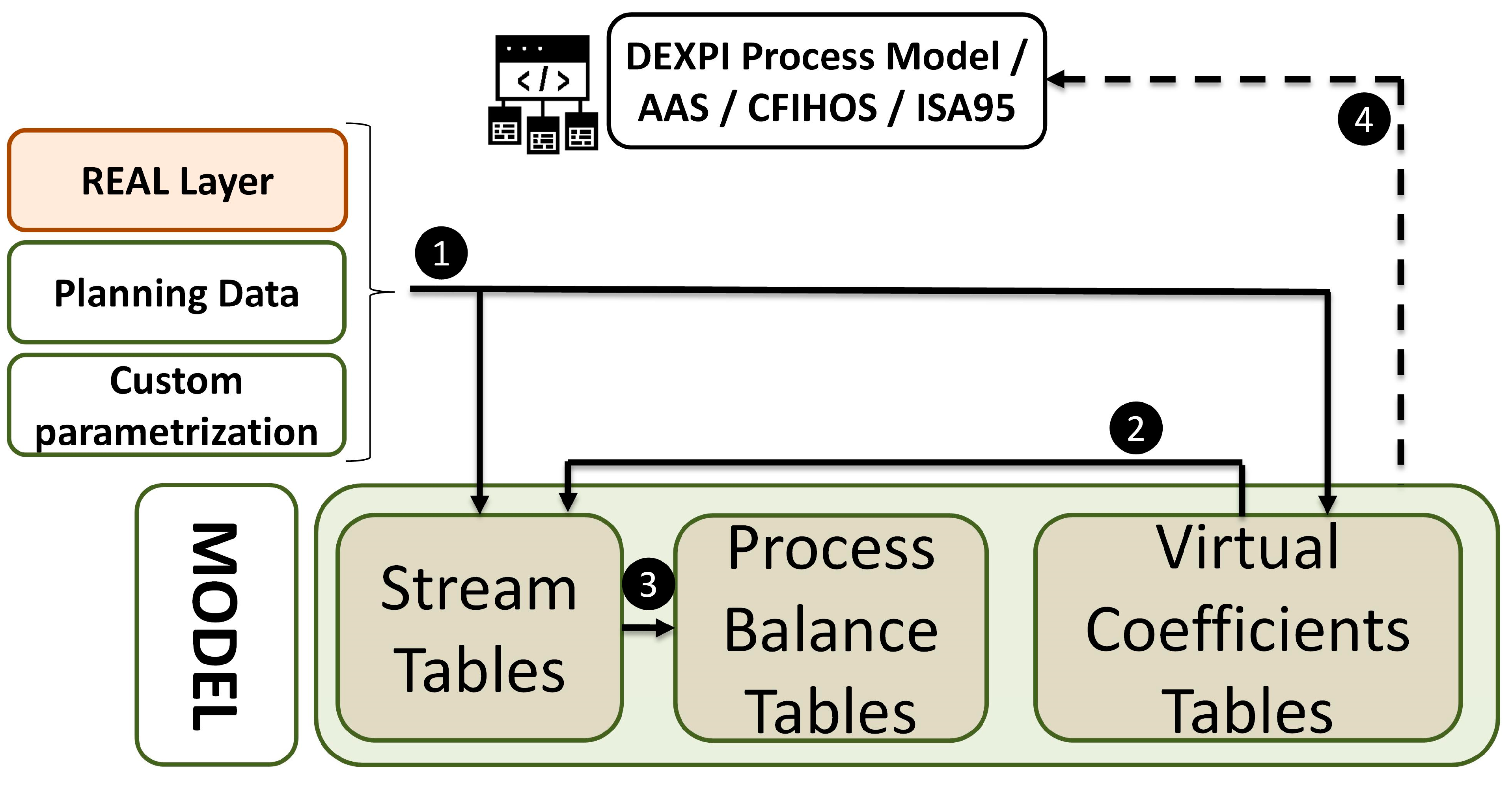
The last (but not least) layer—MODEL—is a virtual representation of the process state based on Inlet stream properties and Virtual Coefficient values. Initial numbers for Inlet streams might be taken directly from the REAL layer, reflecting the operational, planning or manually modified data by the end user (Figure 9, point (1)). A similar aproach is applicable for Virtual Coefficient Tables. Additionally, at this point, the VMB concept provides a space for the implementation of more sophisticated statistics, machine learning algorithms or other solutions which might provide the most suitable values of soft sensors. Their role is to calculate the remaining process streams based on feedstock data. Calculations are also customizable and realized in steps on demand or parallel to the REAL Layer (Figure 9, point (2)). Depending on the considered process, providing the set points of an additional process variable could be applicable and useful. The results of this layer could be compared with REAL values and treated as a benchmark. The third phase of the layer’s development is the calculation of Process Balance Tables (Figure 9, point (3)), which are essentially consistent with other layers. The selected results might enrich the enterprise data model (Figure 9, point (4)).

The exemplary TEP process would take the property values of streams #1, #2, #3 and #4 and estimate others using Virtual Coefficients. Both types would be taken from the REAL layer.

4.4. VMB User Interface

As previously mentioned, the concept should also include the end user interface. There are many tools which might help instantiate the VMB concept. Figure 10, Figure 11, Figure 12, Figure 13 and Figure 14 present the possible implementation of a previously described solution based on the AVEVA PI System (PI System Explorer 2023 Patch 1 and PI Vision 2022 3.7.0.0) commonly used in the process industry.

Figure 10 is an example of a Human–Machine Interface (HMI) visualization which could be dedicated to TEP. All available process variables are shown as current process values, based on an existing dataset [50]. Process monitoring for engineering personnel is limited to the available OT elements.

One of the navigation panes leads to the Stream Table window (Figure 11), where a comparison of Stream properties (as per Figure 4) might be performed. Such data allow for instant understanding and visualization of process data and benchmarking against design values and/or predicted values within the MODEL Layer. The table in the REAL layer without enrichment would be filled only partially, as per Figure 8.

Balance Tables are focused on unit balance and its Process Step sub-balances. Engineers could identify the source of possible misbalance at a glance (Figure 12).

The set of Coefficient Tables presents available values of soft sensors assigned to particular Process steps (Figure 13).

In order to allow users to manipulate MODEL hyper-parameters, there is another dedicated screen (Figure 14) which allows for user interaction with the model to perform different prediction scenarios. The user can decide if the Inlet stream component flows would be assumed as operating values or set manually. Furthermore, the solution allows for the manipulation of coefficients (taken as actual operating values by default). It would be possible to implement advanced algorithms in order to predict them based on selected process variables.

4.5. VMB Concept Classification

In the authors’ opinion, the presented concept can be characterized by the taxonomy of Digital Twins for simulation applications according to van der Valk, Hunker and Rabe’s work, as shown in

Table 1. Taxonomy of simulation models according to van der Valk, Hunker and Rabe [19]. Sign “X” means the variant is applicable to VMB according to the authors.

Dimension		Characteristic	VMB Fitting
D1	Progress over time	Continuous
		Discrete	X
D2	Probability	Deterministic
		Stochastic	X
D3	Nature of the model	Static model	X
		Dynamic model
D4	Process model	Applied	X
		Not applied
D5	Scope of the simulation model	Single-asset
		Multi-asset	X
D6	Verification and validation	Conducted	X
		Not conducted
D7	Time horizon	Finite	X
		Infinite

.

Trying to define the corresponding archetype, the following characteristics can be assigned to the taxonomy of Digital Twins. However, it should be noted that the concept itself does not specify several solutions. In principle, however, it does not exclude their implementation; they depend on corporate rules and the final business purpose. For

Table 2. Characteristics of the dimensions describing VMB according to the taxonomy for Digital Twins [18]. Shaded area is organization-dependent and thus might vary from case to case. Sign “x” means the variant is applicable for VMB according to the authors. Sign “*” means potential characteristics for VMB.

Meta-Dimension	Dimension	Characteristic	VMB Fitting
Data collection	Data acquisition	Automatic	x
		Semi-automatic
	Data sources	Many sources	x
		Single source
	Synchronization	Present	x
		Lack
	Input data	Raw data
		Processed data	x
Data handling and distribution	Data governance	Compliant with the rules	*
		Non-compliant with the rules
	Data communication	Two-way	*
		One-way
	Interface	HMI	*
		M2M	*
	Data reusability	Lack
		Medium	*
		Full
	Objective	Operational	x
		Intermediation
		Repository	x
Conceptual scope	Accuracy	High
		Partial	x
	Components of twins	Independent
		Linked	x
	Creation period	Digital first	x
		Physical first	x
		Simultaneously	x

, the grey items of the “Data handling and distribution” meta-dimension depend on organizational conditions—beyond the considerations of the concept—and an asterisk denotes potential characteristics for VMB.

Considering the “assumed” characteristics, according to the authors’ research, the model with the characteristics indicated in Table 2 can be classified according to the AT2 archetype, i.e., “Enriched Digital Twin”.

5. Discussion

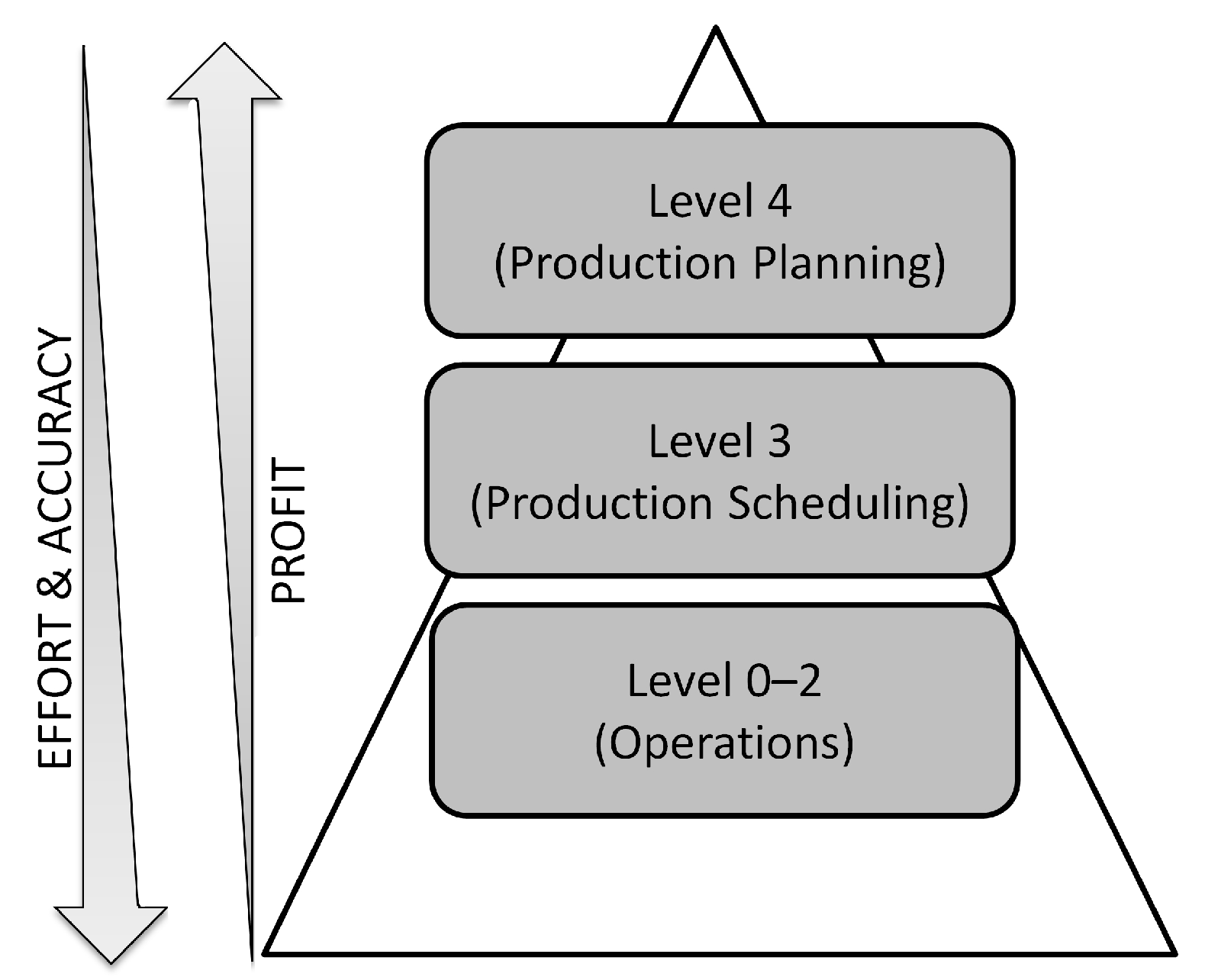
5.1. VMB Across Organizational Structure

Thanks to the moderate complexity of use of PFDs, the concept could be applied by both operation staff and schedulers or planners. Examples of applications for daily monitoring addressed for levels 0–2 (Figure 1) are as follows:

-

Tracking catalyst/reaction performance and comparing different catalyst campaigns;

-

Tracking significant imbalances in stream flows across the unit;

-

Identifying sources of quality issues for streams;

-

Comparing different time periods of operations (for example, during test runs);

-

Tracking separation efficiency and possible relevant places for optimization;

-

Tracking the source of gaps between plan and production;

-

Performing fast and simple what-if analysis for many purposes.

Examples of application for higher levels (schedulers and SCM) are as follows:

-

Back-casting process and LP model improvement;

-

Performing fast and simple what-if analysis for many purposes;

-

Using Virtual Coefficients as KPIs (even for maintenance departments);

-

Developing the VMB for a broader range of process units, which might be feasible due to the moderate complexity and simplicity;

-

Quick shifting between modelled time ranges in the MODEL layer.

Some features, such as the comparison of different time periods, predictions of stream flows and yields and LP model improvements, have already been tested by authors in petrochemical process plants with successful results.

5.2. VMB Among Other Solutions

Nowadays, the term Digital Twin is very popular across industries, and two main trends can be identified: Asset Digital Twins, perfectly reflecting asset documentations and status and characterized by very difficult and time-consuming implementation projects but with broad range of applicability, and Operational Digital Twins, which allow for process monitoring and prediction capabilities. The latter are easier to develop but usually very specific in terms of application. Virtual Mass Balance, on the one hand, might be placed closer to Operational DT, but on the other hand, it presents broader applicability while still having a moderate level of complexity.

The concept itself allows for process monitoring capabilities. The very simple, common and functional visualization layer, by its self-explanatory nature, allows for broad adoption not only across operation staff but also for people not directly involved in the production process. As the literature review shows, there are a number of solutions which support monitoring activities, even though they require very specific expertise [49] and mathematical understanding or have specific applicability [50]. Neither showed benchmarking capabilities against engineering or historical data.

In terms of process modelling and prediction possibilities, typical Operational Digital Twins were presented [53,54,56], but they were built based on deterministic models using chemo-physical rules and properties provided by Downs and Vogel [15] or their derivatives. In most real processes, such model conditions are rarely encountered and process fluctuations might cause GIGO effects. VMB is a mathematical model with stochastic probabilities. The solution is intended to develop a model based on the available process or design data supported by data engineering enrichment. Other solutions possibly related to AI methods [11] are rather black-box and thus difficult to interpret and tune.

Some authors have used the modular approach [44,46], but the presented concepts are significantly different and are not related to any existing standards. VMB utilizing the DEXPI Process model is focused on two main modules (Process Steps): separating (and its specializations) and chemical reactions.

6. Conclusions

Virtual Mass Balance, the newly proposed concept, is a solution that combines data engineering and data modelling, deploying design and historical operational data to determine soft sensors by using the authors’ distribution or reaction coefficients:

-

The presented concept could be classified as an Operational Digital Twin; nevertheless, the utilization of the DEXPI Process standard offers an opportunity for seamless integration with Asset Digital Twin solutions.

-

Some features of Virtual Mass Balance have already been tested by authors on real petrochemical units.

-

Virtual Mass Balance exhibits good flexibility, as evidenced by its implementation using an example from the literature and information limited to the source publication.

-

The simplicity of the application layer and its reliance on the moderate level of detail of Process Flow Diagrams allow the solution to be used both in production areas (monitoring, benchmarking, prediction) and at higher organizational levels (back-casting, predictions).

-

The use of presented soft sensors has not been described in the literature so far. In fact, their use can be assessed after performing a series of engineering transformations/calculations.

References

- Balaji, K.; Rabiei, M.; Suicmez, V.; Canbaz, C.H.; Agharzeyva, Z.; Tek, S.; Bulut, U.; Temizel, C. Status of Data-Driven Methods and their Applications in Oil and Gas Industry. In Proceedings of the SPE Europec Featured at 80th EAGE Conference and Exhibition, Copenhagen, Denmark, 11–14 June 2018; Society of Petroleum Engineers: Richardson, TX, USA, 2018; p. D031S005R007, ISBN 978-1-61399-606-5. [Google Scholar]
- Ren, J. Artificial Intelligence for Refiners. 2018. Available online: https://www.digitalrefining.com/article/1002251/artificial-intelligence-for-refiners (accessed on 18 March 2024).
- Shang, C.; You, F. Data Analytics and Machine Learning for Smart Process Manufacturing: Recent Advances and Perspectives in the Big Data Era. Engineering 2019, 5, 1010–1016. [Google Scholar] [CrossRef]
- Sircar, A.; Yadav, K.; Rayavarapu, K.; Bist, N.; Oza, H. Application of machine learning and artificial intelligence in oil and gas industry. Pet. Res. 2021, 6, 379–391. [Google Scholar] [CrossRef]
- Lee, H.; Sohn, I. Fundamentals of Big Data: Network Analysis for Research and Industry; John Wiley & Sons: Chichester UK; Hoboken, NJ, USA, 2015; ISBN 978-1-119-01549-9. [Google Scholar]
- Bai, C.; Dallasega, P.; Orzes, G.; Sarkis, J. Industry 4.0 technologies assessment: A sustainability perspective. Int. J. Prod. Econ. 2020, 229, 107776. [Google Scholar] [CrossRef]
- Liu, X.; Lu, D.; Zhang, A.; Liu, Q.; Jiang, G. Data-Driven Machine Learning in Environmental Pollution: Gains and Problems. Environ. Sci. Technol. 2022, 56, 2124–2133. [Google Scholar] [CrossRef] [PubMed]
- Jasiulewicz-Kaczmarek, M.; Antosz, K.; Zhang, C.; Ivanov, V. Industry 4.0 Technologies for Sustainable Asset Life Cycle Management. Sustainability 2023, 15, 5833. [Google Scholar] [CrossRef]
- Ning, Y.; Kazemi, H.; Tahmasebi, P. A comparative machine learning study for time series oil production forecasting: ARIMA, LSTM, and Prophet. Comput. Geosci. 2022, 164, 105126. [Google Scholar] [CrossRef]
- Niaei, A.; Towfighi, J.; Khataee, A.R.; Rostamizadeh, K. The Use of ANN and the Mathematical Model for Prediction of the Main Product Yields in the Thermal Cracking of Naphtha. Pet. Sci. Technol. 2007, 25, 967–982. [Google Scholar] [CrossRef]
- Zhang, X.; Zou, Y.; Li, S.; Xu, S. A weighted auto regressive LSTM based approach for chemical processes modeling. Neurocomputing 2019, 367, 64–74. [Google Scholar] [CrossRef]
- Plehiers, P.P.; Symoens, S.H.; Amghizar, I.; Marin, G.B.; Stevens, C.V.; Van Geem, K.M. Artificial Intelligence in Steam Cracking Modeling: A Deep Learning Algorithm for Detailed Effluent Prediction. Engineering 2019, 5, 1027–1040. [Google Scholar] [CrossRef]
- Wang, Y.; Zhang, Y.; Li, H. Adapted Receptive Field Temporal Convolutional Networks with Bar-Shaped Structures Tailored to Industrial Process Operation Models. Ind. Eng. Chem. Res. 2020, 59, 5482–5490. [Google Scholar] [CrossRef]
- Ochoa-Estopier, L.M.; Jobson, M.; Smith, R. Operational optimization of crude oil distillation systems using artificial neural networks. Comput. Chem. Eng. 2013, 59, 178–185. [Google Scholar] [CrossRef]
- Downs, J.J.; Vogel, E.F. A plant-wide industrial process control problem. Comput. Chem. Eng. 1993, 17, 245–255. [Google Scholar] [CrossRef]
- Van Der Valk, H.; Haße, H.; Möller, F.; Otto, B. Archetypes of Digital Twins. Bus. Inf. Syst. Eng. 2022, 64, 375–391. [Google Scholar] [CrossRef]
- Aivaliotis, P.; Georgoulias, K.; Arkouli, Z.; Makris, S. Methodology for enabling Digital Twin using advanced physics-based modelling in predictive maintenance. Procedia CIRP 2019, 81, 417–422. [Google Scholar] [CrossRef]
- Tao, F.; Xiao, B.; Qi, Q.; Cheng, J.; Ji, P. Digital twin modeling. J. Manuf. Syst. 2022, 64, 372–389. [Google Scholar] [CrossRef]
- Van Der Valk, H.; Hunker, J.; Rabe, M.; Otto, B. Digital Twins in Simulative Applications: A Taxonomy. In Proceedings of the 2020 Winter Simulation Conference (WSC); IEEE: Orlando, FL, USA, 2020; pp. 2695–2706. [Google Scholar]
- Harper, K.E.; Malakuti, S.; Ganz, C. Digital Twin Architecture and Standards. IIC J. Innov. 2019, 1–12. [Google Scholar] [CrossRef]
- Zezulka, F.; Marcon, P.; Vesely, I.; Sajdl, O. Industry 4.0—An Introduction in the phenomenon. IFAC-PapersOnLine 2016, 49, 8–12. [Google Scholar] [CrossRef]
- Pada, G. Meet data-centric engineering: Engineering better relationships and more sustainable capital projects. Aveva: Cambridge, UK.
- Cameron, D.B.; Otten, W.; Temmen, H.; Hole, M.; Tolksdorf, G. DEXPI process: Standardizing interoperable information for process design and analysis. Comput. Chem. Eng. 2024, 182, 108564. [Google Scholar] [CrossRef]
- Cameron, D.B.; Otten, W.; Temmen, H.; Tolksdorf, G. DEXPI Process Modelling of Process Systems and their Documentation. Available online: https://dexpi.org/wp-content/uploads/2023/12/DEXPI-Process-1.0-Manual.pdf (accessed on 6 August 2024).
- DEXPI Process Information Model, version 1.0.; DEXPI Initiative: Frankfurt, Germany, 2023.
- Fjøsna, E.; Saltvedt, T.; Waaler, A.; Knædal, M.; Koppergård, V.; Hella, L.; Skjæveland, M.G.; Mehmandarov, R.; Fekete, M.; Zhou, B. Information Modelling Framework Manual (Version 2.1). Available online: https://www.imfid.org/docs/IMF_Manual_v2-1.pdf (accessed on 6 August 2024).
- ISO TC184/SC4 Standing Document; Technical Committee 184 for Industrial Automation Systems and Integration; Subcommittee 4 for Industrial Data. ISO: Geneva, Switzerland, 2021.
- ISO 23247; Automation Systems and Integration—Digital Twin Framework for Manufacturing. ISO: Geneva, Switzerland, 2021.
- CFIHOS Standard; Capital Facilities Information Hand-Over Specification. IOGP: London, UK, 2024.
- ISO 15926; Industrial Automation Systems and Integration—Integration of Life Cycle Data for Process Plants Including Oil and Gas Production Facilities. ISO: Geneva, Switzerland, 2023.
- ISO 14306; Industrial automation systems and integration—JT file format specification for 3D visualization. ISO: Geneva, Switzerland, 2017.
- ISA88; Batch Control. International Society of Automation (ISA): Durham, NC, USA, 2010.
- ISA95; Enterprise-Control System Integration. International Society of Automation (ISA): Durham, NC, USA, 2018.
- IEC PAS 63088:2017; Smart manufacturing—Reference architecture model industry 4.0 (RAMI4.0). IEC: Geneva, Switzerland, 2017.
- Guerra, O.J.; Le Roux, G.A.C. Improvements in Petroleum Refinery Planning: 1. Formulation of Process Models. Ind. Eng. Chem. Res. 2011, 50, 13403–13418. [Google Scholar] [CrossRef]
- Tsay, C.; Baldea, M. 110th Anniversary: Using Data to Bridge the Time and Length Scales of Process Systems. Ind. Eng. Chem. Res. 2019, 58, 16696–16708. [Google Scholar] [CrossRef]
- Lyman, P.R.; Georgakis, C. Plant-wide control of the Tennessee Eastman problem. Comput. Chem. Eng. 1995, 19, 321–331. [Google Scholar] [CrossRef]
- Ricker, N.L.; Lee, J.H. Nonlinear model predictive control of the Tennessee Eastman challenge process. Comput. Chem. Eng. 1995, 19, 961–981. [Google Scholar] [CrossRef]
- Banerjee, A.; Arkun, Y. Control configuration design applied to the Tennessee Eastman plant-wide control problem. Comput. Chem. Eng. 1995, 19, 453–480. [Google Scholar] [CrossRef]
- Duvall, P.M.; Riggs, J.B. On-line optimization of the Tennessee Eastman challenge problem. J. Process Control 2000, 10, 19–33. [Google Scholar] [CrossRef]
- Jockenhövel, T.; Biegler, L.T.; Wächter, A. Dynamic optimization of the Tennessee Eastman process using the OptControlCentre. Comput. Chem. Eng. 2003, 27, 1513–1531. [Google Scholar] [CrossRef]
- Golshan, M.; Boozarjomehry, R.B.; Pishvaie, M.R. A new approach to real time optimization of the Tennessee Eastman challenge problem. Chem. Eng. J. 2005, 112, 33–44. [Google Scholar] [CrossRef]
- Golshan, M.; Pishvaie, M.R.; Bozorgmehry Boozarjomehry, R. Stochastic and global real time optimization of Tennessee Eastman challenge problem. Eng. Appl. Artif. Intell. 2008, 21, 215–228. [Google Scholar] [CrossRef]
- Bauer, M.; Chioua, M.; Schilling, J.; Sand, G.; Harjunkoski, I. Profitability and Re-usability: An Example of a Modular Model for Online Optimization. IFAC Proc. Vol. 2009, 42, 756–761. [Google Scholar] [CrossRef]
- Tătulea-Codrean, A.; Fischer, J.; Engell, S. A Multi-stage Economic NMPC for the Tennessee Eastman Challenge Process. IFAC-PapersOnLine 2020, 53, 6069–6075. [Google Scholar] [CrossRef]
- Setiawan, R.; Hioe, D.; Bao, J. Plantwide Operability Analysis based on a Network Perspective: A Study on the Tennessee Eastman Process. IFAC Proc. Vol. 2010, 43, 451–456. [Google Scholar] [CrossRef]
- Zhang, C.; Guo, Q.; Li, Y. Fault Detection in the Tennessee Eastman Benchmark Process Using Principal Component Difference Based on K-Nearest Neighbors. IEEE Access 2020, 8, 49999–50009. [Google Scholar] [CrossRef]
- Bathelt, A.; Jelali, M. Comparative Study of Subspace Identification Methods on the Tennessee Eastman Process under Disturbance Effects. In Proceedings of the 5th International Symposium on Advanced Control of Industrial Processes, Hiroshima, Japan, 28–30 May 2014. [Google Scholar]
- Heo, S.; Lee, J.H. Statistical Process Monitoring of the Tennessee Eastman Process Using Parallel Autoassociative Neural Networks and a Large Dataset. Processes 2019, 7, 411. [Google Scholar] [CrossRef]
- Kini, K.R.; Madakyaru, M. Improved Process Monitoring Strategy Using Kantorovich Distance-Independent Component Analysis: An Application to Tennessee Eastman Process. IEEE Access 2020, 8, 205863–205877. [Google Scholar] [CrossRef]
- Martin-Villalba, C.; Urquia, A.; Shao, G. Implementations of the Tennessee Eastman Process in Modelica. IFAC-PapersOnLine 2018, 51, 619–624. [Google Scholar] [CrossRef]
- Bathelt, A.; Ricker, N.L.; Jelali, M. Revision of the Tennessee Eastman Process Model. IFAC-PapersOnLine 2015, 48, 309–314. [Google Scholar] [CrossRef]
- Han, C.; Huang, S.; Sun, W. Python platform for Tennessee Eastman Process. In Computer Aided Chemical Engineering; Elsevier, 2022; Volume 49, pp. 889–894. ISBN 978-0-323-85159-6. [Google Scholar]
- He, R.; Chen, G.; Dong, C.; Sun, S.; Shen, X. Data-driven digital twin technology for optimized control in process systems. ISA Trans. 2019, 95, 221–234. [Google Scholar] [CrossRef] [PubMed]
- Reinartz, C.; Kulahci, M.; Ravn, O. An extended Tennessee Eastman simulation dataset for fault-detection and decision support systems. Comput. Chem. Eng. 2021, 149, 107281. [Google Scholar] [CrossRef]
- Iraola, E.; Nougués, J.M.; Chanona, A.D.R.; Batet, L.; Sedano, L. Hybrid data-driven and first principles monitoring applied to the Tennessee Eastman process. In Computer Aided Chemical Engineering; Elsevier: Amsterdam, The Netherlands, 2023; Volume 52, pp. 1803–1808. ISBN 978-0-443-15274-0. [Google Scholar]
- Yélamos, I.; Méndez, C.; Puigjaner, L. Enhancing dynamic data reconciliation performance through time delays identification. Chem. Eng. Process. Process Intensif. 2007, 46, 1251–1263. [Google Scholar] [CrossRef]
- Rieth, C.A.; Amsel, B.D.; Tran, R.; Cook, M.B. Additional Tennessee Eastman Process Simulation Data for Anomaly Detection Evaluation. Harv. Dataverse 2017. [Google Scholar] [CrossRef]
- Bakdi, A.; Kouadri, A. An improved plant-wide fault detection scheme based on PCA and adaptive threshold for reliable process monitoring: Application on the new revised model of Tennessee Eastman process. J. Chemom. 2018, 32, e2978. [Google Scholar] [CrossRef]