Abstract
In the power system, the integration of power-to-gas and carbon capture systems (P2G-CCS) within the microgrid enables the conversion of electrical energy into hydrogen or methane while simultaneously capturing CO2 emissions from power generation units. This approach significantly mitigates carbon emissions and supports the transition to a low-carbon energy system. Concurrently, the dynamic properties of the gas–thermal network exert a critical influence on the flexibility of system scheduling and the regulation of multi-energy coupling. Hence, this paper puts forward an optimal configuration strategy for microgrids with consideration of the dynamic characteristics of the gas–thermal network. Firstly, mathematical models for the dynamic characteristics of the gas network and the heat network were established and incorporated into the microgrid system. Secondly, in conjunction with the P2G-CCS coupling system, an optimization scheduling strategy was formulated with the aim of minimizing the total operational costs of the power grid, the natural gas network, and the heat network. An enhanced African vultures optimization algorithm (AVOA) was put forward. In the end, by setting different scheduling scenarios for conducting a comparative analysis, an appropriate optimization configuration scheme was selected, and the validity of the proposed method was verified through simulation with the improved case study.
1. Introduction
Microgrids play an important role in grid dispatch and reducing environmental pollution. Devices such as power-to-gas and carbon capture systems (P2G-CCS), combined heating and power (CHP), and gas boilers (GBs) in the system have achieved multi-energy complementarity and effectively enhanced energy utilization efficiency [1,2,3,4]. In the electricity–gas–heat multi-energy coupled system, the dynamic characteristics of the gas flow and thermal energy flow can be equivalent to the system standby, which has the ability to improve system flexibility and promote the consumption of new energy [5,6,7,8,9]. Therefore, fully exploiting the regulatory potential of the network dynamic characteristics in the multi-energy coupled system is an effective approach to promote the accommodation of renewable energy and improve the level of system dispatch.
The dynamic characteristics of gas and heat networks have a direct impact on the operational flexibility and optimal scheduling of integrated energy systems. In an electricity–gas–heat integrated energy system, accounting for these dynamic characteristics can substantially enhance both the system’s operational adaptability and its capacity to accommodate renewable energy sources. Existing literature indicates that scholars have already initiated research into the dynamic behaviors of gas and heat networks. Refs. [10,11] proposed a dispatch model of the electric–gas coupled system considering the dynamic characteristics of the gas network, demonstrating that the dynamic characteristics of the gas network can increase the accommodation of new energy and energy utilization efficiency. Ref. [12] constructed a multi-time scale dynamic optimization dispatch model of the coupled electric–gas interconnection system. The case study indicates that the gas pipeline storage makes the output of generating units and gas sources smoother. Ref. [13] approximated the nonlinear dynamic equation of the gas network by a matrix and constructed a two-stage robust dispatch model of the electric–gas coupled system, enhancing the wind power accommodation of the natural gas network.
The P2G-CCS coupled system, as a low-carbon technology, fully taps the potential of the system for the accommodation of new energy. Ref. [14] unified the electrolyzer and the methanation process and applied it in multi-microgrids, achieving the maximization of the benefits of the microgrid clusters. Ref. [15] put forward the concept of the low-carbon operation domain, effectively quantifying the low-carbon operation range of the P2G-CCS system. Ref. [16] combined the carbon trading strategy with the P2G-CCS coupled system and gas-hydrogen blending units, enhancing the economy and low-carbon nature of the virtual power plant. Intelligent algorithms such as genetic algorithm (GA), particle swarm optimization (PSO), and interior search algorithm (ISA) are prone to premature convergence and low accuracy when addressing the optimal configuration of microgrids [17,18,19].
The African vultures optimization algorithm (AVOA) is an optimization algorithm that mimics the behaviors of African vultures during their foraging process, such as hunger, exploration, conflict, and flight. It is formed through the sharing of information and possesses strong optimization capabilities and robustness [20]. Nevertheless, in the initial stage of evolution, due to factors such as insufficient population diversity and alterations in the regulation parameters of cognitive and social behaviors, when optimizing a small portion of multi-extreme value functions, phenomena like deteriorated population convergence accuracy or even local convergence are prone to occur [21,22].
To sum up, in this paper, an optimal configuration strategy for microgrid considering the dynamic characteristics of gas and heat is proposed, and an economic optimal configuration model of microgrid is established. By establishing the mathematical model of gas and heat dynamic characteristics and integrating it into the microgrid system, the level of system dispatch decision-making is enhanced. By integrating the P2G-CCS coupled system to mitigate carbon emissions and applying the Levy flight strategy to the AVOA to solve the objective function, the aim is to enhance the solution accuracy and convergence speed, thereby attaining the optimal solution.
2. Dynamic Characteristics of Gas and Heat Networks
2.1. Dynamic Characteristics of Gas Networks and Modeling
When focusing on the dynamic characteristics of the gas pipeline networks, the transmission speed of natural gas during its transmission in the pipelines is relatively slow and it is compressible. This leads to the gas flow at the inlet and outlet of the pipelines not being equal. The portion of natural gas that lingers in the gas network pipelines is referred to as “pipe inventory”. It can be expressed as [23]:
where and are the length and diameter of pipeline , respectively, with their units being km and m, while the unit for pipeline is km. is the natural gas inventory of pipeline at time period , the unit of time t is h, and the unit for gas inventory within the pipeline is kg/s. is the natural gas constant, Tg is the temperature of natural gas, and the unit for the temperature of natural gas is °C. The compressibility factor of natural gas is designated as and the density of natural gas is specified as under the standard atmospheric pressure, kg/m3. constitutes the average pressure of pipeline nl within period , and the unit of pressure is MPa. The pressures at node and node are indicated in MPa by and , respectively. During the time period , the gas flow rates entering and exiting the pipeline are and , respectively, the unit of time t is h, and the unit for the gas flow rate is kg/s.
By substituting Equation (2) into Equation (1), further calculations yield the relationship between pipe inventory and node pressure:
Just as the standby in the power system, the pipeline inventory in the gas network is capable of mitigating the fluctuations of the natural gas load and constitutes a crucial factor for ensuring the reliable supply of natural gas [23]. Based on the physical properties of natural gas, which behaves as an incompressible fluid, maintaining a specific pressure during pipeline transportation is essential to ensure optimal flow efficiency. This characteristic complicates rapid adjustments to the gas supply volume. To effectively manage pipeline storage and ensure smooth operation in the subsequent scheduling cycle, the pipeline inventory at the end of each cycle is set to match the initial inventory level [23]:
where is the set of natural gas pipelines, and and represent the pipeline inventories at the outset and conclusion of a scheduling period, respectively.
2.2. Dynamic Characteristics and Modeling of the Thermal Network
The dynamic characteristics of the thermal network are mainly manifested in the influence on the temperature variation of the medium, which is reflected in the two aspects of transmission delay and temperature loss. In this paper, the water flow in the network remains unchanged, and only the temperature variation of the thermal network is considered; that is, we employ the control mode characterized by constant flow and variable temperature.
- (1)
- Transmission Delay
When taking into account the transmission delay characteristics, the temperature loss is not considered. The exit temperature of the pipe can be estimated by using the temperature at the pipe inlet and the transmission delay characteristics of the pipe during a certain period of time. The delay constants and are expressed as follows [4]:
where is the flow rate of hot water of the pipeline in period , the unit for time is h, and the unit for flow rate is kg/s. At time and time , the retention time values of the portion of hot water flowing out from the pipeline are designated as and , respectively, and the units for both and are denoted in h. , , and are the density of hot water, the cross-sectional area of the hot water pipeline , the length of the hot water pipeline , and the total mass of hot water, respectively, while the units for density, cross-sectional area, length, and mass are kg/m3, m2, km, and kg, respectively; . In the circumstance where the temperature loss is disregarded, this article utilizes a linear weighting methodology to characterize the outlet temperature of the pipe, and the unit for the outlet temperature of the pipeline is °C. The expression for the outlet temperature of the pipeline is given as follows [4]:
In Equations (8) and (9)
where and are the outlet temperatures of the supply water pipe line and the return water pipeline , respectively, without temperature loss in period . The unit of time t is h and the unit for the outlet temperature is °C. Within the ambit of the time period , the inlet temperatures of the supply water pipe hl and the return water pipe hl are designated as and , respectively, and the unit for the inlet temperature is °C. From the time period to the time period , the mass of hot water entering the pipe hl is defined as , the unit for the time period is defined as h, and the unit for the mass of hot water is kg. Within the interval extending from time to time , the mass of hot water entering pipe hl is defined as , the unit for the time period is defined as h, and the unit for the mass of hot water is kg.
- (2)
- Temperature loss
During the course of hot water transmission within pipes, heat loss occurs as a consequence of heat exchange between the hot water and the pipe wall. Subsequently, considering the heat loss, the outlet temperature of the pipe can be calculated in accordance with the Shukhov formula. The detailed formulas are provided as follows [6]:
where and are the outlet temperatures after considering the temperature loss, °C; is the temperature loss coefficient; is the ambient temperature, °C; and is the thermal conductivity of the pipeline . The specific heat capacity of water is denoted by the letter , J/(kg·°C).
3. Microgrid
3.1. Unit Model
- (1)
- P2G-CCS Coupling Model
Power-to-gas (P2G) technology facilitates the conversion of electrical energy into gaseous energy carriers such as hydrogen or methane, which can subsequently be stored within existing natural gas infrastructure or dedicated storage facilities. Carbon capture and storage (CCS) technologies encompass three primary CO2 capture methods: pre-combustion carbon capture, post-combustion carbon capture, and oxy-fuel combustion. Among these, post-combustion carbon capture is the most widely implemented approach due to its compatibility with current industrial processes.
Based on the operational characteristics of P2G and CCS, it is evident that relying solely on CCS equipment presents significant challenges. Due to the current limitations in carbon capture and storage technologies, CO2 transportation over long distances pose a risk of leakage and incurs substantial costs. Conversely, utilizing only P2G systems necessitates the procurement of CO2 for methanation processes, thereby increasing overall system expenses. Therefore, integrating P2G and CCS technologies can enhance the economic viability of the system while simultaneously reducing CO2 emissions.
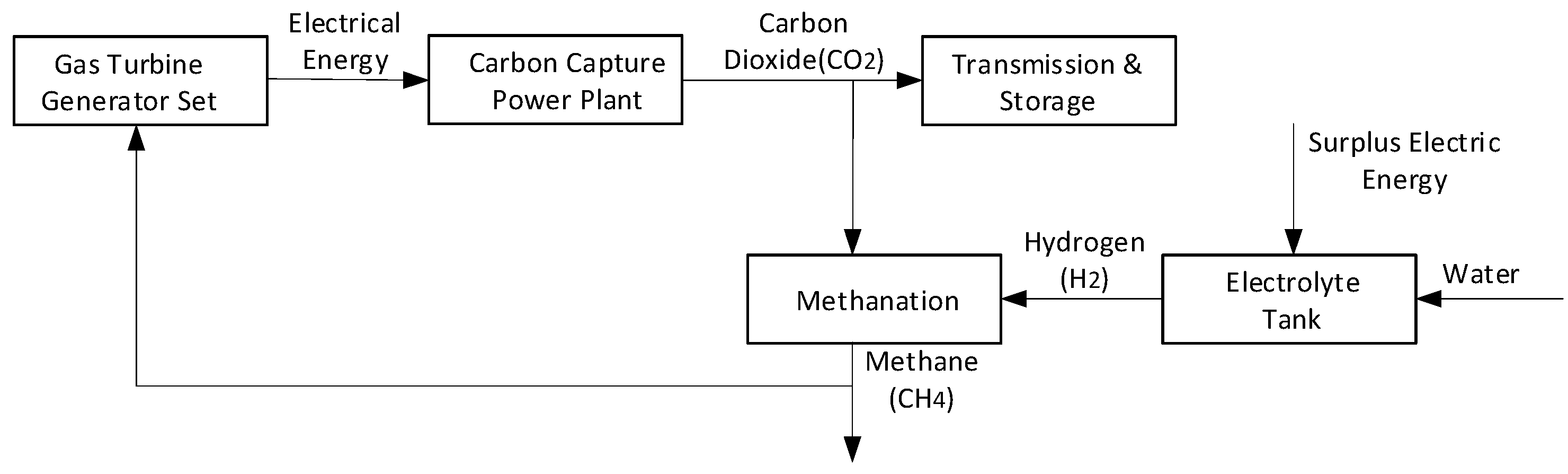
As illustrated in Figure 1, CCS technology captures CO2 from the flue gas emitted by fossil fuel-fired power units. Following separation and purification, the captured CO2 is transported to the methane reactor. Concurrently, an electrolyzer produces hydrogen through water electrolysis, which subsequently reacts with the captured CO2 to generate methane. The synthesized methane is then injected into the natural gas pipeline network to serve as a feedstock for gas turbines, thereby facilitating the recycling and efficient utilization of energy.
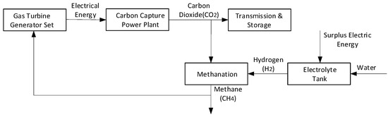
Figure 1.
Working principle of the integrated operation of P2G and CCS.
The CO2 generated by the CHP unit and the electricity purchased from the external power grid can be captured by the P2G-CCS system, thus achieving energy conservation and emission reduction, and improving economic benefits. The P2G-CCS system model is presented as follows [21]:
In Equation (15), represents the gas production power of P2G, kW; represents the power consumption of P2G, kW; represents the power consumption of CCS, kW; represents the capture amount of CO2, kg; represents the efficiency of electricity-to-gas conversion of P2G; represents the electricity consumption for processing per unit mass of CO2; and represents the electricity consumption for capturing per unit mass of CO2.
- (2)
- Electric Boiler Model [21]
- (3)
- Gas Turbine Model
The gas turbine can realize the transformation from the chemical energy in natural gas to electricity. The mathematical model of the gas turbine is [24]:
where denotes the gas consumption power of the gas turbine, kW; indicates the power generation of the gas turbine, kW; represents the heat production power of the gas turbine, kW; represents the gas-to-electricity efficiency of the gas turbine; and represents the gas-to-heat efficiency of the gas turbine.
- (4)
- Gas Boiler Model [24]
- (5)
- Energy Storage Battery Model [5]
- (6)
- Output Power Model of Photovoltaic Array
In view of the relatively low power output of each individual photovoltaic cell, multiple photovoltaic cells are integrated into photovoltaic modules via series or parallel connections. Subsequently, photovoltaic arrays are constituted in the same way to augment the overall photovoltaic power generation capacity. The expression for the output power of photovoltaic power generation is as follows [5]:
In Equation (20), under standard test conditions (STC), the maximum test power is defined as , kW, within which denotes irradiance, W/m2, represents the temperature of the photovoltaic power generation system, °C, and refers to the power temperature coefficient. In actual operating conditions, the irradiance is A, W/m2, and the surface temperature of the photovoltaic panel is , °C.
- (7)
- Output Power Model of Wind Turbine
In conditions where the wind rotor coefficient, swept area of the rotor, and air density are held constant, the output power of the wind turbine is fundamentally dependent on wind speed and demonstrates a cubic relationship with it. The mathematical representation for the output power of the wind turbine is as follows [25]:
where , , is the rated power of the wind turbine, kW; is the wind speed at the hub height of the wind turbine, m/s; is the cut-in speed, m/s; and is the cut-out speed, m/s. The output power of the wind turbine amounts to when the rated wind speed is and the units for and are kW and m/s, respectively. can be obtained through the following formula [25]:
where is the output power of the wind turbine when the wind speed is and the units for and are kW and m/s, respectively.
3.2. Objective Function
The objective function of the integrated energy system (IES) is comprised of three distinct components: the operational cost associated with the power grid , the operational cost related to the natural gas network , and the operational cost pertaining to the heating network . The cost units for each term in the objective function are uniformly denominated in US dollars [16].
3.2.1. Grid Operating Costs
The objective function of the power grid is formulated based on a comprehensive economic cost model that employs the concept of equal annual value while also incorporating environmental considerations into the objective function in terms of costs. This approach facilitates the resolution of a nonlinear programming problem under specified constraints. The components of this objective function encompass equivalent initial investment costs, fuel expenditures, environmental costs associated with electricity generation, as well as the expenses related to purchasing and selling electricity. This model can be expressed as follows [16]:
where represents the total cost, while N denotes the number of unit categories, with the total cost unit specified in US dollars. denotes the equivalent initial investment cost per unit of installed capacity for the i-th type of generating unit, US dollars; represents the operational and maintenance costs associated with the i-th type of generating unit, US dollars; signifies the fuel cost per unit of electricity generated by diesel generators, US dollars; indicates the environmental cost per unit of electricity generation from diesel generators, US dollars; refers to the electricity output from the i-th type of generating unit, kWh, while pertains to the electricity output from diesel generators, kWh. Additionally, and represent the purchase and sale prices of electricity over a specified period, the pricing unit is specified in US dollars, whereas and denote the quantities of purchased and sold electrical energy during that same period, the unit of measurement for electrical energy is specified as kWh. Each item carries a weight of 1.
- (1)
- Equivalent Initial Investment Cost
The initial investment cost is determined using the equivalent method, and the model is articulated as follows [8]:
where denotes the unit price of the i-th type of generator, US dollars; represents the operational lifespan of the i-th type of generator, y; and signifies the discount rate.
- (2)
- Operating and Maintenance Costs
The operating and maintenance costs of the unit are comprised of fixed costs and variable costs. The mathematical model is articulated as follows [10]:
where and , respectively, denote the fixed operation and maintenance expense and the variable operation and maintenance expense of the i-th generating unit, US dollars.
- (3)
- Fuel Expenditure
The combustion of fuel in diesel The operation of the unit requires fuel consumption, and the corresponding fuel costs are incorporated into the calculation of economic expenses. The model representing the fuel cost per unit of electricity generated by this unit is formulated as follows [10]:
where denotes the unit price of fuel required for power generation by the diesel generator, US dollars, while represents the fuel consumption per unit of electricity produced by the diesel generator, kg.
- (4)
- Annual Environmental Cost of Power Generation
The combustion of fuel in diesel generators for electricity generation results in CO2 emissions. When these emissions are converted into environmental costs and integrated into the calculation of economic costs, the model can be articulated as follows [16]:
where denotes the type of gas emitted during the power generation process of diesel generators; signifies the environmental assessment standard for pollutants within the power industry; and represents the quantity of the i-th pollutant emitted per unit of electricity generated by the diesel generator.
3.2.2. Operating Costs of the Gas Network
Operating costs associated with the natural gas network [17].
where denotes the set of natural gas sources, and and represent the output from the gas source and the unit price of natural gas during period . The unit of time t is h, and the unit of measurement for the unit price of natural gas is dollars/m3.
3.2.3. Operating Costs of the Heating Network [17]
3.3. Constraints
3.3.1. Power Grid Constraints
- (1)
- Power Balance Constraints [18]
- (2)
- Node Power Balance Constraint [18]
- (3)
- Constraints on Power Flow in Transmission Lines [19]
- (4)
- Phase Angle and Generator Output Constraints [19]
- (5)
- Constraints of Generator Ramp [23]
3.3.2. Constraints of the Gas Network and the Heat Network
The static model of the natural gas system incorporates node flow balance constraints, gas source output constraints, pipeline gas flow constraints, and node pressure constraints. The dynamic model of the thermal system consists of heat network temperature constraints, heat power balance constraints, outlet temperature constraints of cogeneration units, and inlet temperature constraints of heat exchange stations. For detailed information, please refer to Reference [26]. The dynamic constraints of the gas network and the heat network include Equations (1)–(14).
4. African Vultures Optimization Algorithm (AVOA)
In 2021, Abdollahzadeh et al. proposed the African vultures optimization algorithm (AVOA) through mimicking the foraging behavior of vulture groups in the natural environment [20]. In comparison with other swarm intelligence algorithms, AVOA holds stronger exploration and exploitation capabilities. To a certain degree, this ensures that AVOA does not fall into local optima, maintains a certain convergence rate, and also avoids excessive divergence.
4.1. Stage 1: Ascertainment of the Optimal Vulture for Each Arbitrary Group
Upon the establishment of the initial population, the fitness of all solutions is computed, and the supremely optimal solution is selected as the first group vulture and the second-best optimal solution as the second group vulture, while the residual solutions move towards the first and second groups. During each fitness iteration, the entire population is recalculated [20].
where R(i) designates one of the optimal vultures, constitutes the current position vector of the vultures, L1 and L2 are parameters stipulated prior to the search operation, with their values falling within the range of 0 to 1, and the sum of the two parameters amounts to 1. The probability of selecting the optimal solution is obtained by recourse to the roulette method, and each optimal solution is selected for each group [20].
where Fi indicates the fitness value.
4.2. Stage 2: The Hunger Rate of Vultures
Inspired by the rate at which vultures achieve satiety or experience hunger, the model is presented as follows [20]:
where F represents the satiety rate, Iterationi represents the current iteration number, and maxiterations represents the maximum iteration number. Define z, h, and rand1 as random numbers. Among them, the value of z is any value within the range of −1 to 1, the value of h is any value within the range of −2 to 2, and rand1 is any value ranging from 0 to 1. w is a constant with a value of 2.5. Simultaneously define that when z < 0, the vulture is in a state of hunger, and when z = 0, the vulture is in a state of fullness.
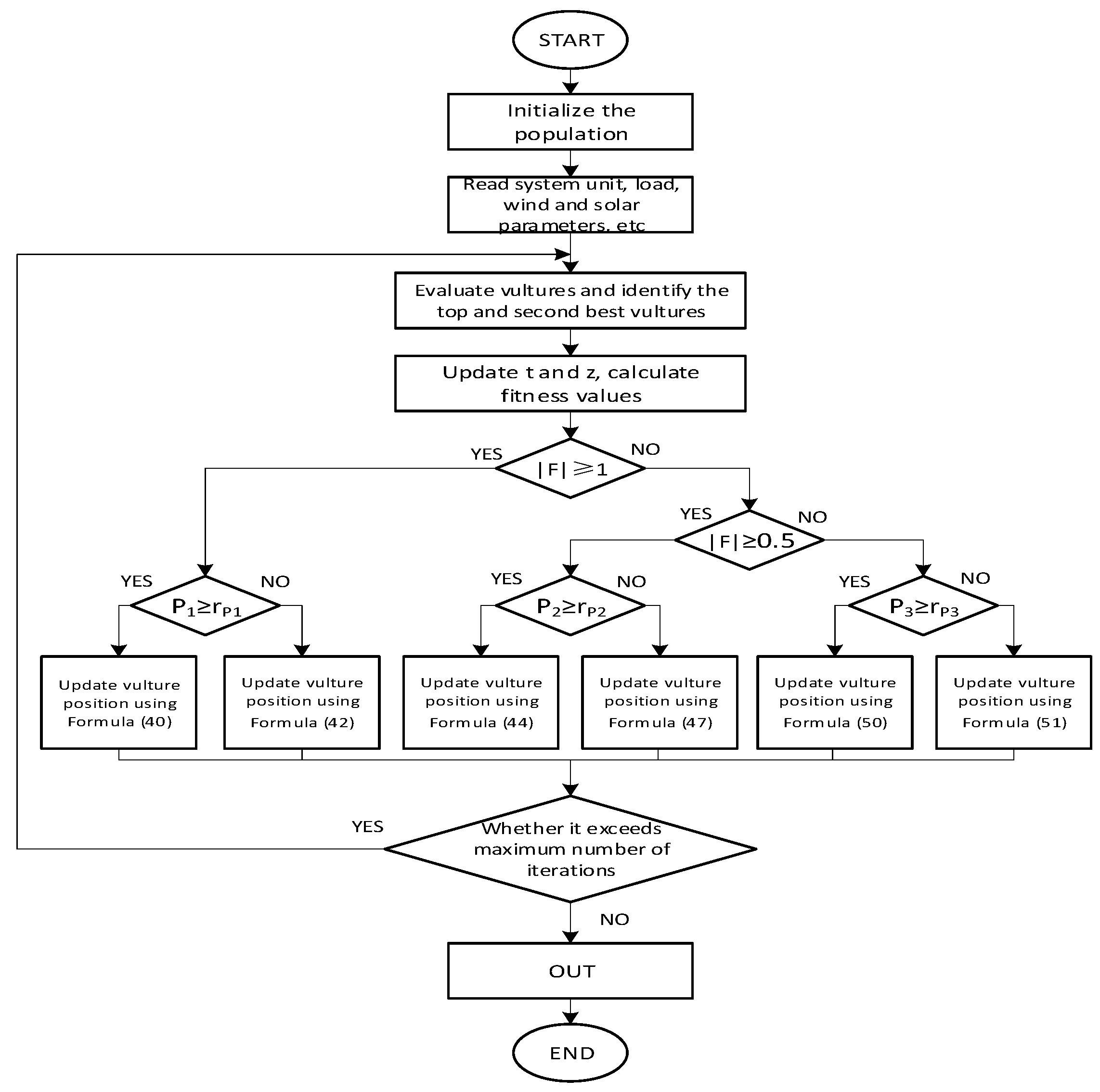
When |F| ≥ 1, the vulture group seeks food in different areas, and at this time, it is defined that AVOA enters the exploration stage. When |F| < 1, the vulture group is in the exploitation mode; that is, it searches for food near the optimal position.
4.3. Stage 3: Foraging Exploration
In the AVOA framework, vultures scrutinize random areas based on two strategies, which are selected through P1. A random number ranging from 0 to 1, namely randP1, is generated. When prevails, formula (40) is utilized; when prevails, Formula (42) is utilized. The search for the satiation region is presented as follows [20]:
where P(i + 1) constitutes the position vector of the vulture subsequent to the iteration, D(i) represents the random distance between the current vulture and one of the superior vultures within the two groups, and X constitutes the random moving position of the vulture, which is obtained by employing the formula in order to safeguard the food from other vultures. To develop a model that generates random solutions within the interval , the following formula is utilized [20]:
In Equation (42), and signify the upper and lower bounds of the variable, and and are random numbers ranging within 0 to 1, employed to augment the randomness coefficient. When approximates 1, a random movement is incorporated into lb to enhance diversity and explore distinct spatial regions.
4.4. Stage 4: Exploitation
When the value of |F| is encompassed within the range of 0.5 and 1, AVOA undertakes two distinct rotational flight and siege strategies. P2 is utilized to determine the selection of each strategy, and its value is within the range of 0 and 1. At the initial phase, a random number randP2 is generated ranging from 0 to 1. When , the siege strategy will be implemented gradually by means of Formula (44). When , the rotational flight strategy is executed by resorting to Formula (47). The formulas are presented as follows [20]:
When |F| ≥ 0.5, the aggregation of a large number of vultures at the same food source may give rise to severe conflicts. Stronger vultures possess a higher likelihood of obtaining food. Weaker vultures cluster around stronger ones, initiating minor conflicts to fatigue them and thereby acquire food. The movement model is presented as follows [20]:
In this formulation, is a random number spanning from 0 to 1, which is employed to augment the random coefficient; denotes the distance between the current vulture and one of the optimal vultures within the two groups.
The rotational flight of vultures is utilized to simulate the spiral motion. Choose one from among the two superior vultures and establish the spiral equation with the remaining ones. The formula is as follows [20]:
where and are random numbers within the range from 0 to 1.
When |F| < 0.5, a random number randP3 within the interval from 0 to 1 is generated. When , several types of vultures accumulate on the food source. When , the siege strategy is adopted. The process is presented as Equation (48) [20].
All the vultures moving towards the food source shall be marked. At this juncture, several distinct types of vultures will accumulate. The movement model is presented as follows [20]:
where BestVulture1(i) constitutes the optimal vulture within the current iteration, and BestVulture2(i) represents the best vulture in the second group during the current iteration.
4.5. Enhancement of the AVOA Algorithm
In this stage, the leading vulture becomes hungry and feeble, and other vultures move to this position for the food search. The movement model is presented as follows [27,28]:
where pertains to the flight mechanism, which is utilized to augment the optimization efficiency of AVOA. The specific expression is depicted as follows [27,28]:
where β equals 1.5, and denote the standard deviations, and ; µ and v represent the direction vectors, which conform to a normal distribution:
In conjunction with fuzzy control, the flowchart of the algorithm is presented in Figure 2.

Figure 2.
Flowchart of the algorithm.
5. Case Analysis
5.1. Unit Parameters
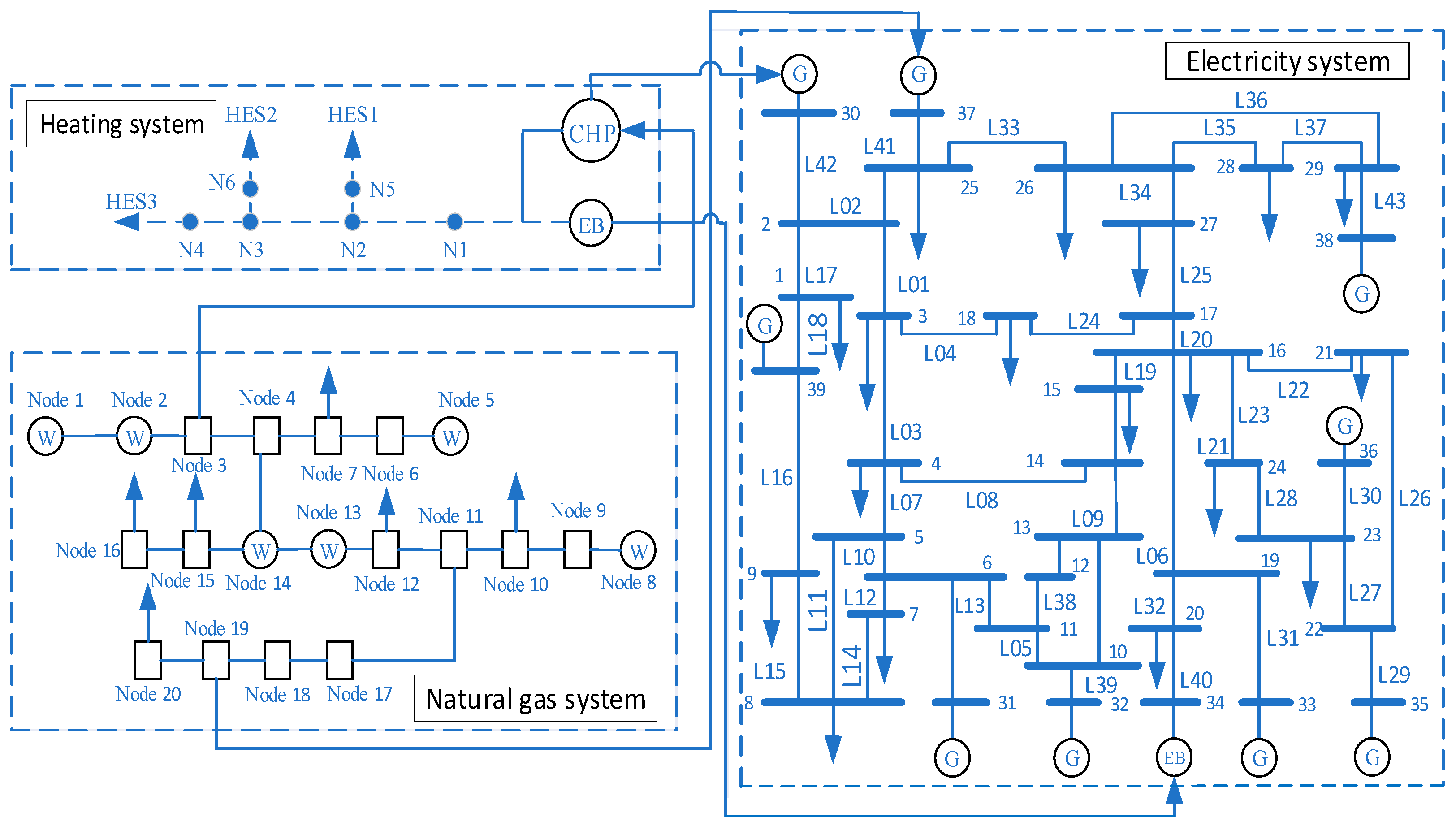
In this paper, a microgrid system is constructed by taking the IEEE-39 node power grid-20 node natural gas network-6 node thermal system as an example. The diagram of the integrated energy system is presented in Figure 3. It encompasses the IEEE-39 bus system, the twenty-node natural gas system in Belgium, and the six-node thermal system. Herein, the generator at Node 30 of the IEEE-39 node power system is configured as a CHP unit, which simultaneously serves as a heat source connected to Node 1 of the six-node thermal system. Node 34 is linked to the EB unit of the thermal system. The natural gas consumed at node 37 is supplied by node 19 within the natural gas distribution network, and the generator at node 37 is configured as a P2G-CCS unit. The 20-node natural gas system in Belgium comprises six gas sources and nine natural gas loads. The heat sources in the six-node thermal system include a CHP unit and an electric boiler, and the electric power consumed by the electric boiler is provided by the CHP unit. To enhance the coupling strength among electricity, gas, and heat, the CHP unit is designated as a gas-fired unit, and the natural gas it consumes is supplied by Node 3 of the natural gas system. The unit cost coefficients, parameters of gas and heat pipelines, etc. are provided in reference [29]. The parameters of diverse types of equipment are presented in Table 1, and the forecast values of wind and solar power are illustrated in Figure 4.
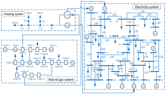
Figure 3.
The topological structure of the integrated energy system.

Table 1.
Parameters of equipment.

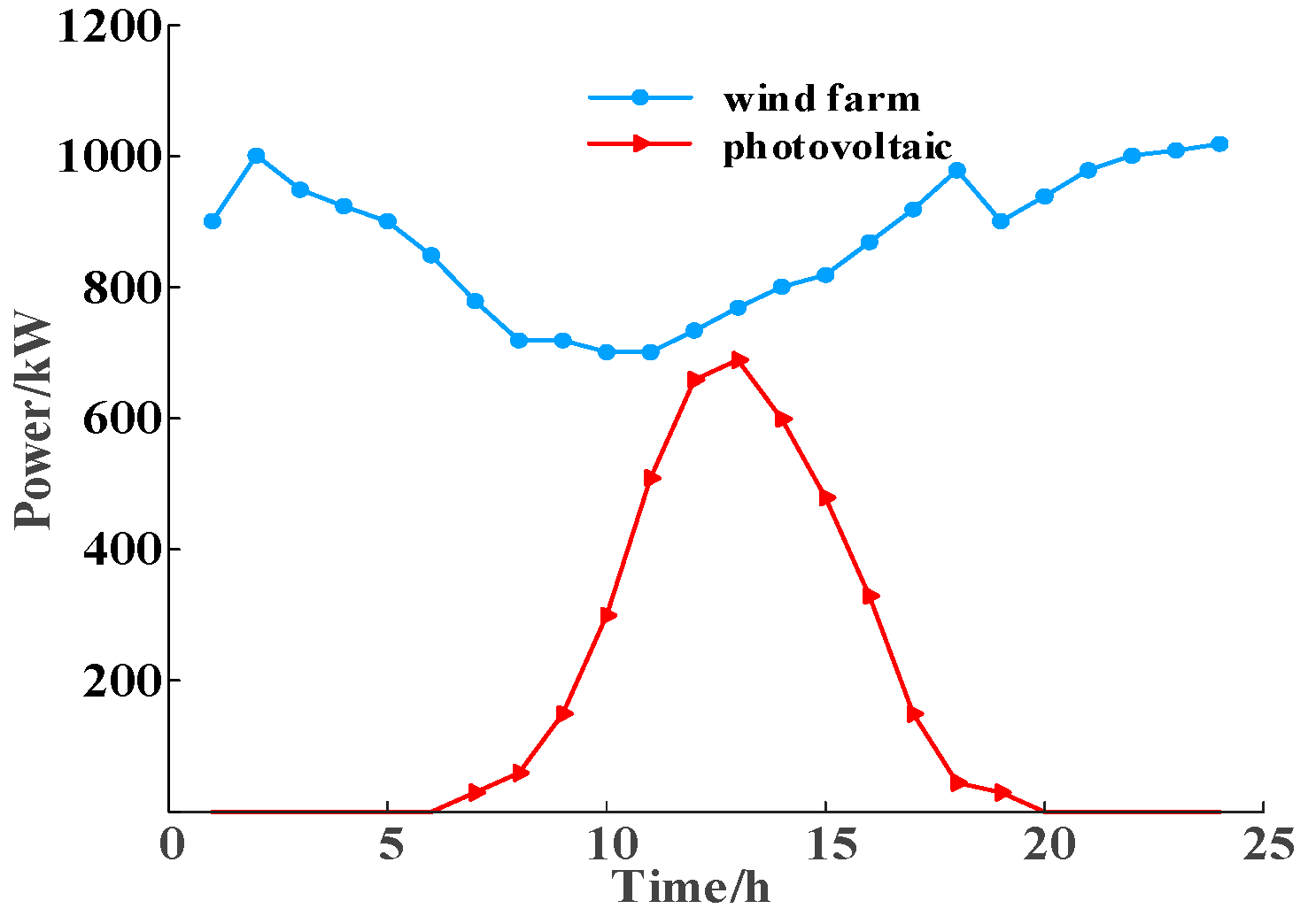
Figure 4.
The forecasted values of wind and solar power.
As illustrated in Figure 4, the power generation from wind energy exceeds that of photovoltaic sources in 24 h. Accurate forecasting of wind and solar power output enables the power system to proactively plan and adapt its operational strategies. This includes optimizing generator configurations and the charge–discharge protocols of energy storage systems, thereby ensuring the stability and reliability of electricity supply. Such predictive data facilitates the maximization of renewable energy utilization and mitigates potential inefficiencies arising from unforeseen weather fluctuations.
5.2. Analysis of the Optimization Scheduling Results for Different Schemes
To assess the influence of the established dynamic model on the gas-hydrogen blending units and system scheduling, the hydrogen blending ratios of CHP and GB are both set at 0.1, and four scenarios are delineated: in Scenario 1, no P2G-CCS coupling equipment is integrated, and the gas–thermal dynamic characteristics are not taken into consideration; in Scenario 2, the P2G-CCS coupling equipment is integrated, but the gas–thermal dynamic characteristics are not considered; in Scenario 3, the gas–thermal dynamic characteristics are accounted for, yet no P2G-CCS coupling equipment is added; and in Scenario 4, the P2G-CCS coupling equipment is integrated, and the gas–thermal dynamic characteristics are taken into account. The scheduling results and unit outputs under different scenarios are respectively presented in Table 2 and Table 3.
Table 2.
Comparison of scheduling results in different scenarios.
Table 3.
Unit output results under different scenarios.
By contrasting Scenario 1 with Scenario 2, the total system cost is reduced by 493.31 dollars. Through the carbon capture equipment, the CO2 generated by the units is collected, the output of the diesel units is decreased, the actual carbon emissions are lower than the carbon quota, and carbon trading benefits are realized. Some of the fuels for CHP and GB are provided by the methanation process, reducing the cost of gas purchase. The electricity consumed by P2G-CCS is supplied by wind and solar power, enhancing the accommodation of wind and solar power, and reducing the penalty cost of new energy. After the addition of the P2G-CCS coupling equipment, the operation and maintenance costs of the units increase.
When comparing Scenario 2 with Scenario 3, the total system cost is reduced by 109.54 dollars. This is because the dynamic characteristics of the gas and heat networks allow energy to be temporarily stored in the pipelines in the form of pipeline storage, and supply gas turbines for peak shaving during the peak period of electrical load. While meeting the electrical load demand, the pipeline storage significantly reduces the output costs of gas and heat sources provided by wind, solar and diesel units. With the increase in the accommodation of wind and solar power, the output of diesel units rises and the coal consumption cost increases.
In contrast to the steady-state circumstances of Scenario 3, the total system cost of Scenario 4 is reduced by 151.29 dollars. Concurrently, taking into consideration the dynamic features of the gas–thermal network can maximize the accommodation capability of renewable energy and enhance the operational flexibility and economic performance of the multi-energy coupling system.
CCS technology captures the carbon dioxide emitted by power generation units and supplies it to P2G systems, thereby reducing both the cost of purchasing natural gas and the carbon emissions from these units. The integration of P2G with CCS not only decreases the system’s overall carbon dioxide emissions and operational costs but also enhances the integration capacity of renewable energy sources. According to Table 3, Scenario 1 exhibits the highest level of carbon emissions. In comparison to Scenario 1, Scenario 2 demonstrates a reduction in carbon emissions. Furthermore, Scenario 4 shows a decrease in carbon emissions due to the incorporation of dynamic factors and control strategies.
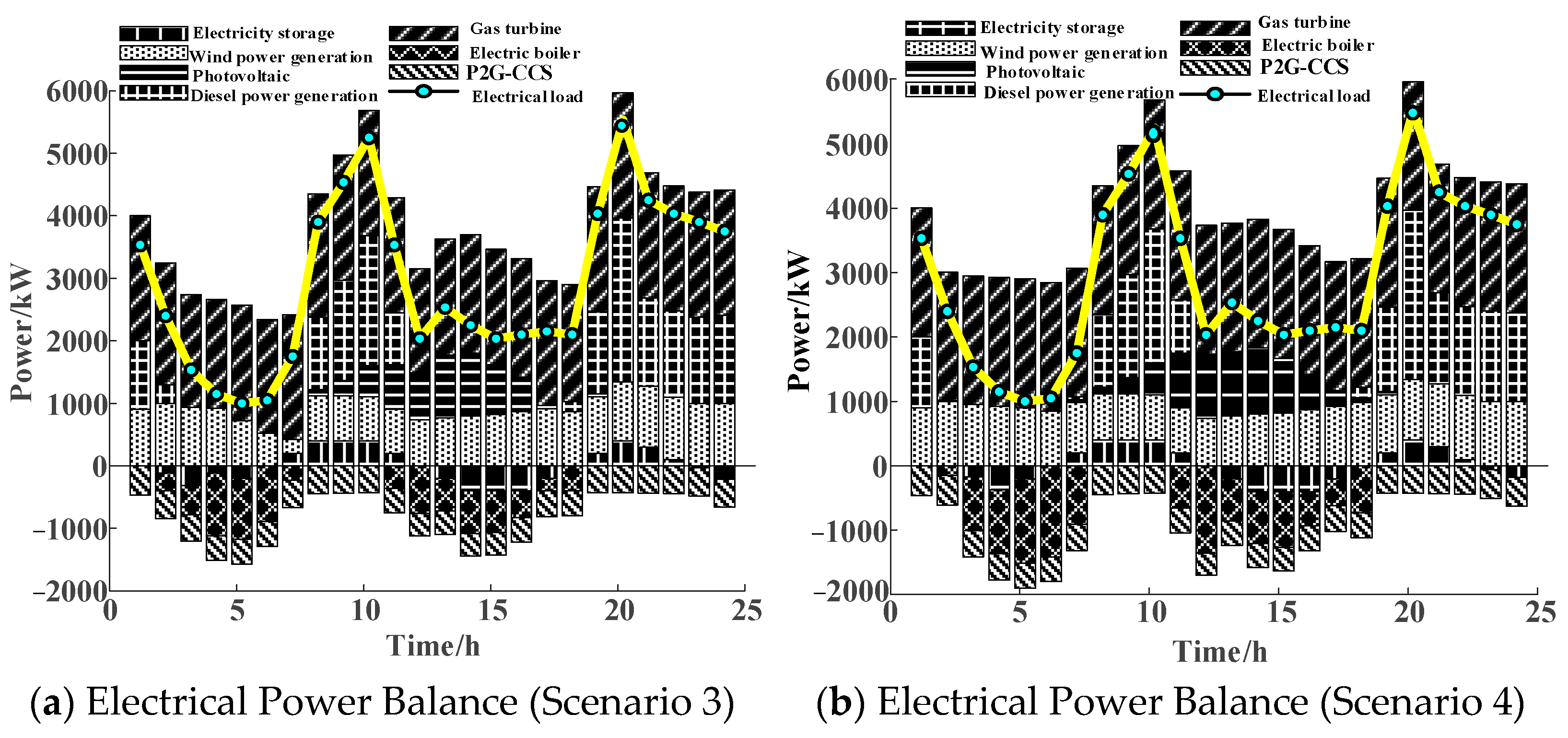
The power balance of the system in Scenario 3 and Scenario 4, respectively, is presented in Figure 5a,b. Taking into consideration the dynamic characteristics of the gas network and the heat network, the output of the diesel-generating unit declines at 01:00, while the output of the wind power generation unit rises at 07:00. In light of the relatively low demand for electrical load during the low electricity consumption period, the power supply requirements of the system can be fulfilled by the CHP and the wind-solar power units. When in the peak electricity consumption period, the output of the diesel-generating unit increases. At this point, the electrical energy is utilized for load supply, the power consumption of the electric boiler is zero, and the heat load is satisfied by the CHP and the GB. Due to the influence of the carbon trading strategy during dispatching, accordingly, in order to reduce carbon emissions, the heat output of the CHP decreases, and the electrical output of the CHP reduces in accordance with the heat-determined electricity strategy.
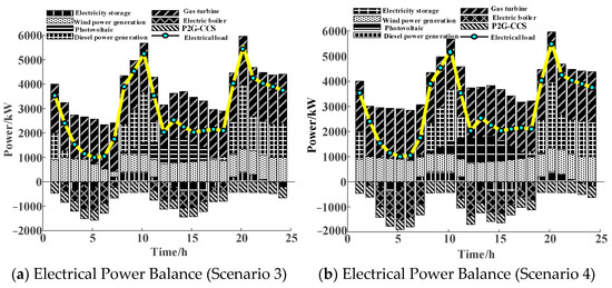
Figure 5.
Electrical power balance in Scenarios 3 and 4.
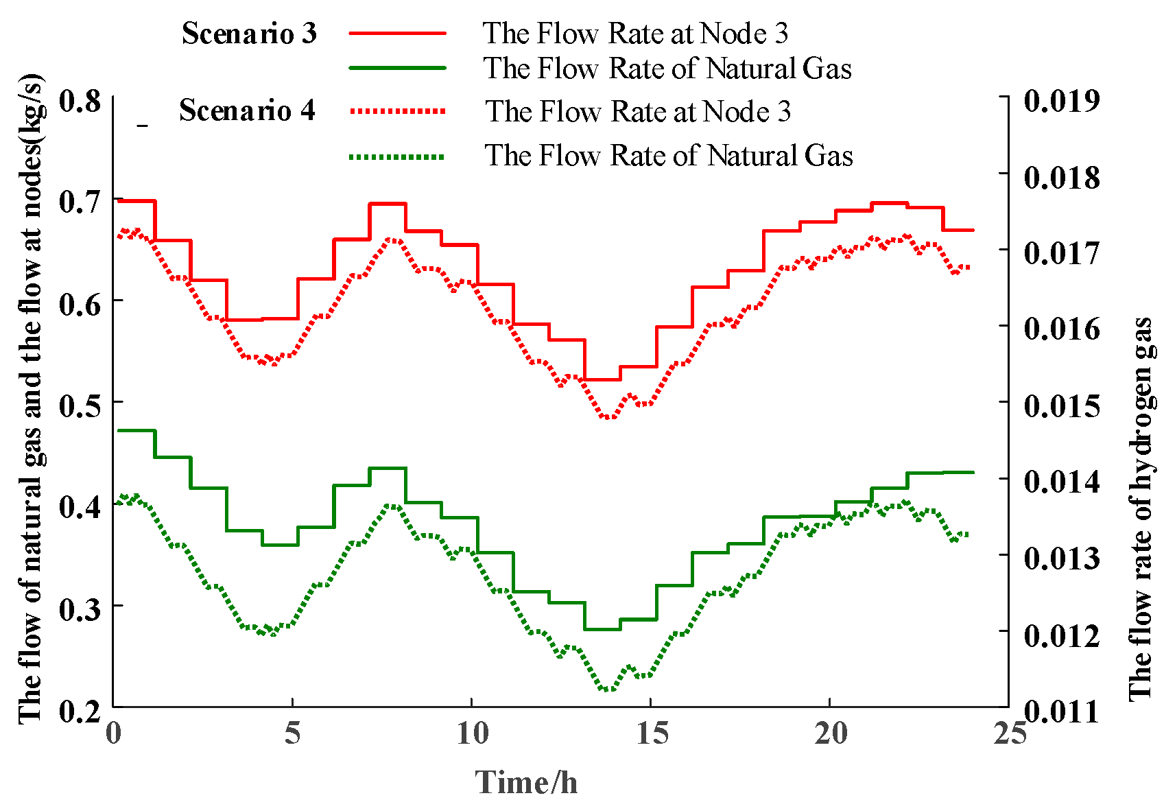
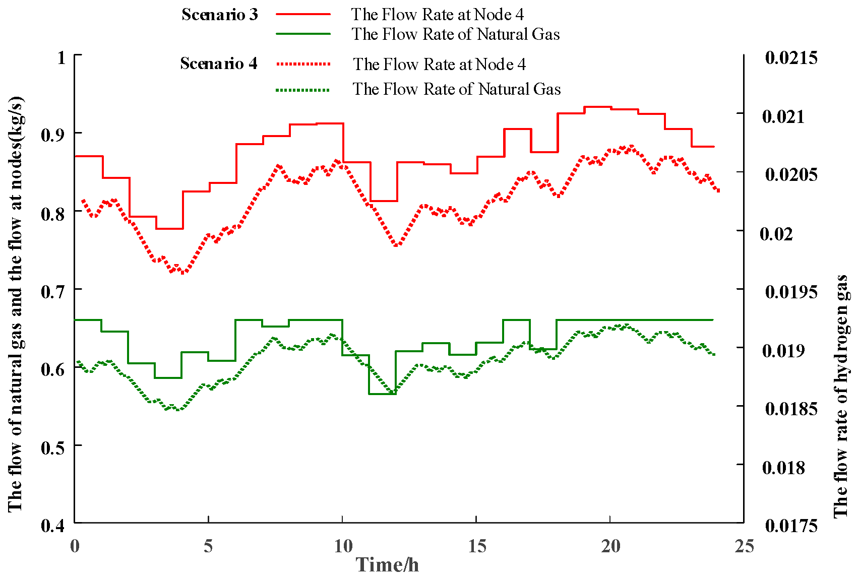
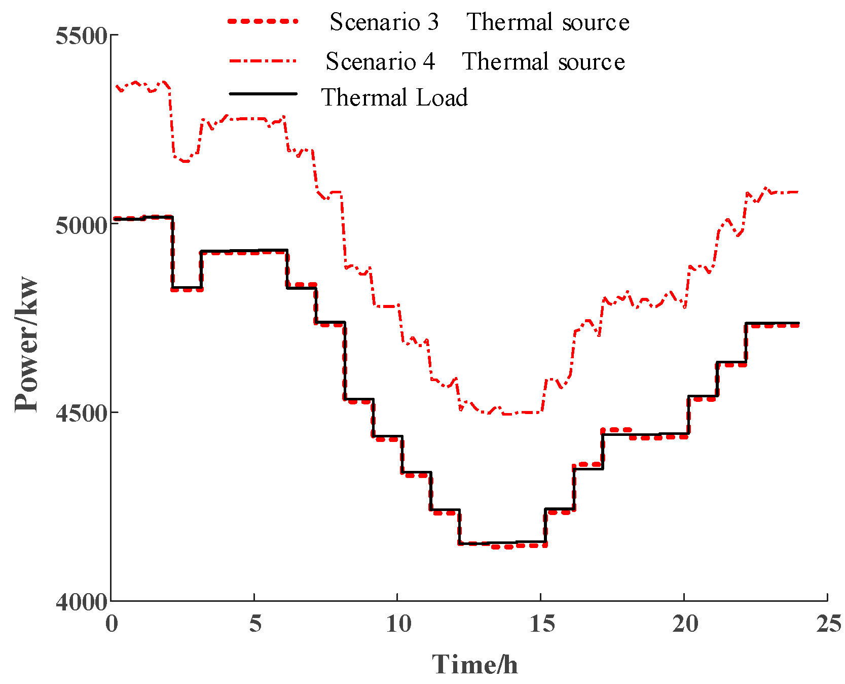
The natural gas consumption of CHP units and GB, as well as the gas flow through the network nodes, are illustrated in Figure 6 and Figure 7, respectively. The heat source output is shown in Figure 8. Compared to Scenario 3, Scenario 4 exhibits a reduction in natural gas flow. This decrease can be attributed to the consideration of dynamic characteristics: when load demand increases, the system leverages the storage capacity of the gas network to reduce gas purchases; conversely, when load demand decreases, the units meet the demand by consuming natural gas, leading to reduced pipeline flow and more stable node flow fluctuations. Considering the thermal losses inherent in the heat distribution network, Scenario 4 requires increased heat source output, which clearly reflects the changes in natural gas flow within the pipeline. Given that CHP units provide both electrical and thermal energy, GB is primarily used for heating to minimize electricity consumption and gas procurement costs, resulting in higher natural gas consumption.
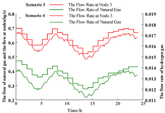
Figure 6.
The consumption of natural gas by gas turbines.
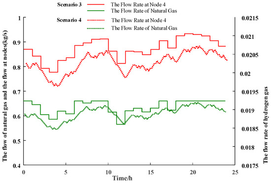
Figure 7.
The consumption of natural gas by gas boilers.
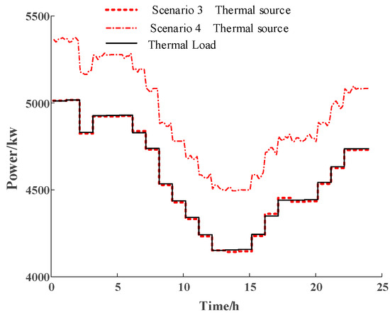
Figure 8.
The output of the heat source.
5.3. Analysis of Algorithm Optimization Outcomes
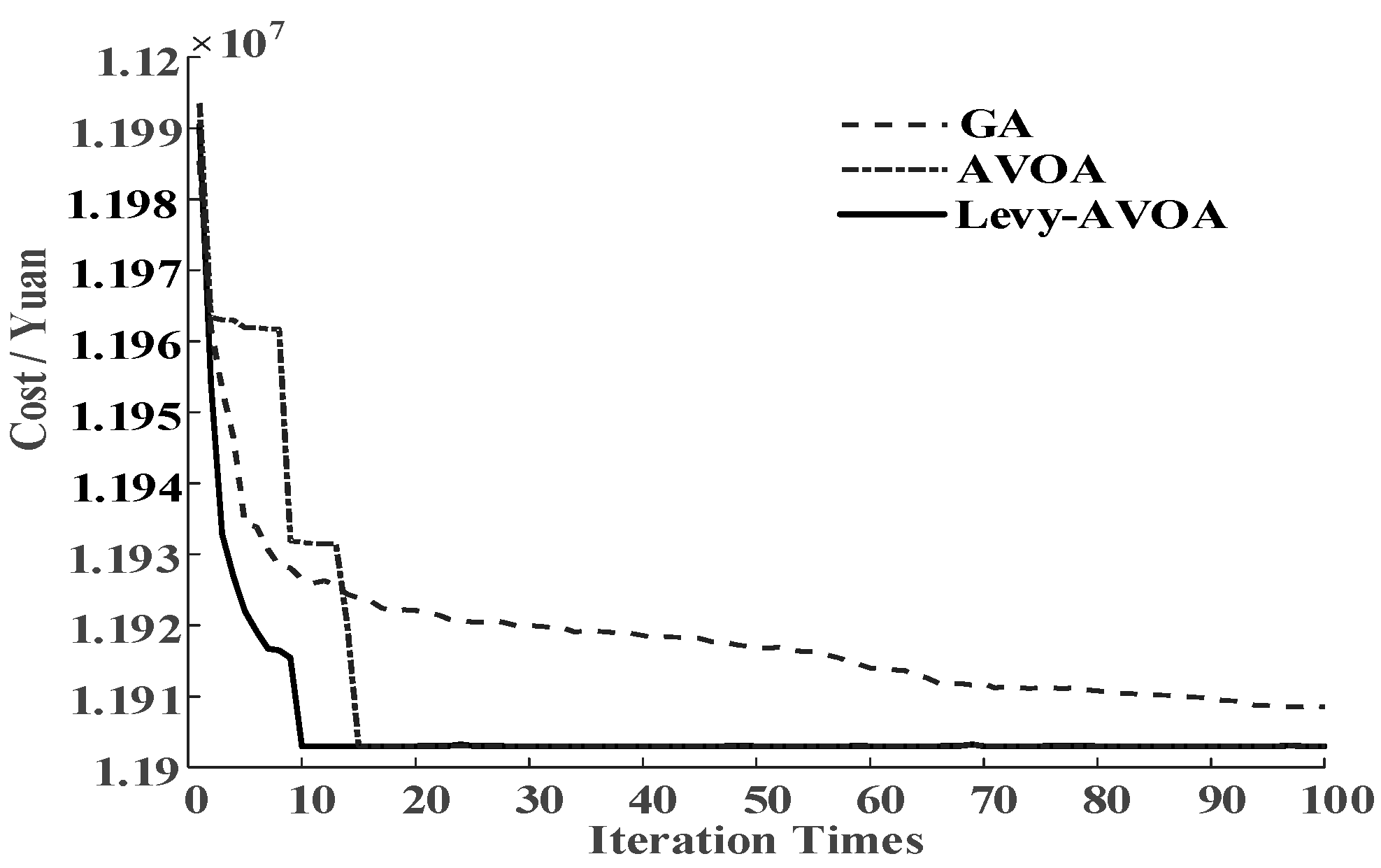
Concerning the convergence effect of the Levy-AVOA algorithm in problem-solving, this paper makes a comparison with the AVOA algorithm and the genetic algorithm (GA) in this respect. The comparison results are presented in Figure 9.
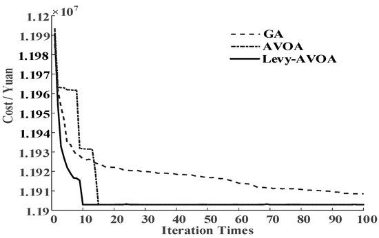
Figure 9.
Comparison of the effects of algorithms.
It can be discerned from the figure that the convergence speed of the Levy-AVOA algorithm surpasses that of other algorithms. Among them, the AVOA algorithm necessitates the assignment of an initial point and possesses relatively high randomness. The GA algorithm exhibits a relatively rapid convergence speed initially, but the convergence speed decelerates as it progresses. The results obtained by employing the Levy-AVOA algorithm can minimize the total operating cost of the microgrid on the premise of meeting the power supply demand, thereby attaining the enhancement of economic benefits.
6. Conclusions
This paper puts forward an optimal microgrid dispatch model, taking into account the dynamic characteristics of the gas–thermal network and the P2G-CCS coupling system. Through the simulation analysis of the electric–gas–thermal network system, the following conclusions are reached:
- (1)
- Through modeling the dynamic characteristics of the natural gas network and the heat network, it is anticipated to enhance the storage capacity inherent in the gas and heat transmission process, and by integrating the flexible energy storage and heat release capabilities of each unit, the level of complementarity and mutual support of the multi-energy coupling system has been further elevated, and the accommodation level of renewable energy has been enhanced.
- (2)
- P2G-CCS exhibits a strong driving force during operation. The combination of the dynamic characteristics of gas and heat and P2G-CCS for joint optimization configuration is conducive to increasing the consumption of wind power and enhancing the economic benefits and energy efficiency utilization ratio of the system.
- (3)
- Compared with the classical heuristic algorithms, the proposed Levy-AVOA algorithm, based on the improved AVOA algorithm, which refers to the Levy flight strategy, is verified through simulation to have a rapid convergence rate and high precision when solving multi-dimensional and nonlinear constraint problems. It is more applicable to solving nonlinear optimization problems.
Author Contributions
F.W. and Z.T. conceived the idea and designed the research, analyzed and interpreted the data, and wrote the paper. All authors have read and agreed to the published version of the manuscript.
Funding
This research received no external funding.
Data Availability Statement
Data are contained within the article.
Conflicts of Interest
The authors declare that they have no known competing financial interests or personal relationships that could have appeared to influence the work reported in this paper.
References
- Li, P.; Yang, M.; Wu, Q. Confidence interval based distributionally robust real-time economic dispatch approach considering wind power accommodation risk. IEEE Trans. Sustain. Energy 2021, 12, 58–69. [Google Scholar] [CrossRef]
- Shi, J.; Wang, L.; Lee, W. Hybrid Energy Storage System (HESS) optimization enabling very short-term wind power generation scheduling based on output feature extraction. Appl. Energy 2019, 256, 113915. [Google Scholar] [CrossRef]
- Zhang, Y.; Zhang, T.; Guo, B. Multi-objective dispatch of a microgrid with battery energy storage system based on model predictive control. Adv. Mater. Res. 2014, 1070–1072, 1384–1390. [Google Scholar] [CrossRef]
- Levihn, F. CHP and heat pumps to balance renewable power production: Lessons from the district heating network in Stockholm. Energy 2017, 137, 670–678. [Google Scholar] [CrossRef]
- Wang, Y.; Zhang, N.; Kang, C. Standardized matrix modeling of multiple energy systems. IEEE Trans. Smart Grid 2019, 10, 257–270. [Google Scholar] [CrossRef]
- Qadrdan, M.; Abeysekera, M.; Chaudry, M. Role of power-to-gas in an integrated gas and electricity system in Great Britain. Int. J. Hydrogen Energy 2015, 40, 5763–5775. [Google Scholar] [CrossRef]
- Shao, C.; Ding, Y.; Wang, J. Modeling and integration of flexible demand in heat and electricity integrated energy system. IEEE Trans. Sustain. Energy 2018, 9, 361–370. [Google Scholar] [CrossRef]
- Li, Z.; Wu, W.; Shahidehpour, M. Combined heat and power dispatch considering pipeline energy storage of district heating network. IEEE Trans. Sustain. Energy 2016, 7, 12–22. [Google Scholar] [CrossRef]
- Meng, Q.; Guan, S.; Jia, N. An improved sequential energy flow analysis method based on multiple balance nodes in gas-electricity interconnection systems. IEEE Access 2019, 6, 95487–95495. [Google Scholar] [CrossRef]
- Zhang, H.; Cheng, Z.; Jia, R. Economic optimization of electric-gas integrated energy system considering dynamic characteristics of natural gas. Power Syst. Technol. 2021, 45, 1304–1311. [Google Scholar]
- Lin, Y.; Shao, Z.; Chen, F. Distributed low-carbon economic scheduling of integrated electricity and gas system based on gas network division. Power Syst. Technol. 2023, 47, 2639–2645. [Google Scholar]
- Mei, J.; Wei, Z.; Zhang, Y. Dynamic optimal dispatch with multiple time scale in integrated power and gas energy systems. Autom. Electr. Power Syst. 2018, 42, 36–42. [Google Scholar]
- Yang, J.; Zhang, N.; Kang, C. Effect of natural gas flow dynamics in robust generation scheduling under wind uncertainty. IEEE Trans. Power Syst. 2017, 33, 2087–2097. [Google Scholar] [CrossRef]
- Wang, K.; Liang, Y.; Jia, R. Two-stage Optimal Scheduling of Nash Negotiation-based Integrated Energy Multi-microgrids With Hydrogen-doped Gas Under Uncertain Environment. Power Syst. Technol. 2023, 47, 3141–3159. [Google Scholar]
- Gao, Y.; Ren, Z.; Jiang, Y. Analysis method of committed carbon emission operational region for electricity-hydrogen coupling system. Electr. Power Autom. Equip. 2023, 43, 29–36. [Google Scholar]
- Chen, D.; Liu, F.; Liu, S. optimization of virtual power plant scheduling coupling with P2G-CCS and doped with gas hydrogen based on stepped carbon trading. Power Syst. Technol. 2022, 46, 2042–2054. [Google Scholar]
- Wu, H.; Zhuang, H.; Zhang, W. Optimal allocation of microgrid considering economic dispatch based on hybrid weighted bilevel planning method and algorithm improvement. Int. J. Electr. Power Energy Syst. 2016, 75, 28–37. [Google Scholar] [CrossRef]
- Trivedi, N.; Jangir, P.; Bhoye, M. An economic load dispatch and multiple environmental dispatch problem solution with microgrids using interior search algorithm. Neural Comput. Appl. 2018, 30, 2173–2189. [Google Scholar] [CrossRef]
- Wang, Q.; Li, K.; Chen, L. Optimization allocation of microgrid capacity based on chaotic multi-objective quantum genetic algorithm. Appl. Mech. Mater. 2011, 22, 71–78. [Google Scholar] [CrossRef]
- Abdollahzadeh, B.; Gharehchopogh, S.; Mirjalili, S. African vultures optimization algorithm: A new nature-inspired metaheuristic algorithm for global optimization problems. Comput. Ind. Eng. 2021, 158, 107408. [Google Scholar] [CrossRef]
- Kumar, C.; Mary, M. Parameter estimation of three-diode solar photovoltaic model using an Improved-African Vulture optimization algorithm with Newton-Raphson method. J. Comput. Electron. 2021, 20, 2563–2593. [Google Scholar] [CrossRef]
- Kumar, P.; Das, C.; Soren, N. Tilt Integral Sliding Mode Control Approach for Real-Time Parameter Variation-Based Frequency Control of Hybrid Power System Using Improved African Vulture Optimization. Arab. J. Sci. Eng. 2024, 49, 15849–15862. [Google Scholar] [CrossRef]
- Fang, J.; Zeng, Q.; Ai, X. Dynamic optimal energy flow in the integrated natural gas and electrical power systems. IEEE Trans. Sustain. Energy 2018, 9, 188–198. [Google Scholar] [CrossRef]
- Schiebahn, S.; Grube, T.; Robinius, M. Power to gas: Technological overview, systems analysis and economic assessment for a case study in Germany. Int. J. Hydrogen Energy 2015, 40, 4285–4294. [Google Scholar] [CrossRef]
- Thapar, V.; Agnihotri, G.; Sethi, K. Critical analysis of methods for mathematical modelling of wind turbines. Renew. Energy 2011, 36, 3166–3177. [Google Scholar] [CrossRef]
- Zhang, Y.; Sun, P.; Ji, X. Dynamic Economic Dispatch for Integrated Energy System Based on Parallel Multi-Dimensional Approximate Dynamic Programming. Autom. Electr. Power Syst. 2023, 47, 60–68. [Google Scholar]
- Amirsadri, S.; Mousavirad, J.; Ebrahimpourkomleh, H. A Levy flight-based grey wolf optimizer combined with back-propagation algorithm for neural network training. Neural Comput. Appl. 2018, 30, 3707–3720. [Google Scholar] [CrossRef]
- Chechkin, V.; Metzler, R.; Klafter, J. Introduction to the theory of Levy flights. In Anomalous Transport: Foundations and Applications; John Wiley Sons: Weinheim, Germany, 2008; pp. 129–162. [Google Scholar]
- Tao, J.; Hong, D.; Lin, B. Optimal energy flow and nodal energy pricing in carbon emission- embedded integrated energy systems. CSEE J. Power Energy Syst. 2018, 4, 179–187. [Google Scholar]
Disclaimer/Publisher’s Note: The statements, opinions and data contained in all publications are solely those of the individual author(s) and contributor(s) and not of MDPI and/or the editor(s). MDPI and/or the editor(s) disclaim responsibility for any injury to people or property resulting from any ideas, methods, instructions or products referred to in the content. |
© 2025 by the authors. Licensee MDPI, Basel, Switzerland. This article is an open access article distributed under the terms and conditions of the Creative Commons Attribution (CC BY) license (https://creativecommons.org/licenses/by/4.0/).