Entropy Generation Modeling in Dynamic Local Thermal Non-Equilibrium Systems Using Neural Networks

Abstract

The study of entropy generation in thermal non-equilibrium (TNE) states has significant implications for optimizing thermal management systems and understanding heat transfer mechanisms in permeable media. This study investigates the entropy properties in a thermal non-equilibrium (TNE) state within double-lid-driven enclosures filled with a permeable medium. Unlike the temperature equilibrium state, the entropy approach is described by two equations: one for the irreversibility of the mixture phase and one for the irreversibility of the medium phase. High mixed convection is considered due to the motion of the non-facing edges (left-side and upper edges). Four cases based on the direction of motion are examined: Case 1, where the left-side and top edges move in the negative and positive directions of the Y- and X-axes, respectively; Case 2, where the upper and left-side edges move in the negative and positive directions of the X- and Y-axes, respectively; and Cases 3 and 4, where the edges move in the positive and negative directions of the respective axes. Heat generation within the flow domain is considered for both the suspension and medium phases. The governing system is solved numerically using finite volume techniques with the SIMPLER algorithm. The obtained data are used to predict key quantities, such as the heat transfer rate, under the influence of major factors using an effective artificial neural network (ANN) analysis. The main findings show that the solid phase entropy is higher in Case 3 compared to the other cases. Additionally, Case 2 results in a minimum solid phase Nusselt coefficient at the center of the active boundary.

1. Introduction

The modeling of flow behavior in permeable media using volume-averaging of the continuity and momentum formulations leads to the characterization of Darcian flow. This type of flow describes fluid transmission through media in terms of viscous resistance. When the solid, fluid, or walls exhibit significant viscous resistance, a mixed mode of flow occurs, resulting in a non-Darcian flow. In a related context, porous media involved in various physical, chemical, and biological processes have solid and fluid phases. The solid matrix of such media possesses certain morphological and chemical properties. These properties make such media different from the homogeneous and isotropic continuum media. Such considerations, therefore, are accounted for to simulate the transport processes at the microscale level, studied in terms of theoretical models, characterized via microscale methods, or seen in terms of technologically protrusive parameters. Furthermore, suspension flow and heat transport processes in natural and renewable porous media or tissue engineering are the core essences of a variety of natural phenomena and biotechnologies. Such natural and renewable porous media are typically adaptively populating and conducting with a mixed mode of flow. The fluid motion and heat transport through permeable materials have been the subject of extensive research in recent decades, due to their many engineering and scientific applications. Some of these applications are the nuclear industry, storage and exchange of thermal energy, packed-bed heat exchangers, geothermal reservoirs and aquifers, catalytic converters, air pollution control, biological systems, thermal insulation of buildings, electron cooling, industrial processes, quality of food, indoor air quality studies, cooling of electronics, automobile thermal comfort, rehabilitation of buildings, solar heating and cooling, fuel cells, etc., for further details see [1,2,3,4,5].

Also, the effects of the Rayleigh number, which is linked to the thermal buoyancy of the nanofluid within the permeable medium, are found to be similar to those of the nanoparticle concentrations and the energy conductivity ratio of the nanoliquid. Higher Rayleigh numbers indicate stronger buoyancy forces, enhancing convective heat transport. It was stated that for nearly the highest porosities, heat transport is enhanced by the inclusion of nanoparticles because of higher thermal conductivity properties. This enhancement is more pronounced at higher nanoparticle concentrations, as the aforementioned property of the nanoliquid increases, improving the overall heat transport values [6,7]. Contrarily, the Nusselt coefficient decreased with the insertion of copper nano-elements in some studies due to the increased pressure drop within the slot. This pressure drop results from the higher density and lower thermal conductivity of copper compared to other materials like clay, which was used in the modeling of the nanoparticles [8]. The balance between the enhanced thermal conductivity and the reduced viscosity plays an important role in determining the overall heat transport efficiency. In the same context, thermophoresis drives nanoparticles from hot to cold regions, promoting a uniform distribution of the temperature and improving heat transport. These mechanisms facilitate the introduction of nanoparticles into the hot fluid boundary layer, increasing the fluid’s heat transfer capability [9]. To study these effects, researchers examined the free convective flow of water–silver nanoliquid in a regular chamber filled with a permeable medium. The cavity’s left-side edge is heated, while other boundaries are adiabatic. This setup helps analyze the influence of parameters like the Rayleigh coefficient, nanoparticle concentration, and thermal conductivity on heat transport characteristics [10,11]. In an investigation presented by Farhad et al. [12], a square geometry was utilized to examine the forced flows of a Cu–water nanoliquid within a regular chamber. The cavity featured a lid that moved regularly along the non-inclined plane, while the remaining boundaries remained stationary. Natural convection was given by heating the left-side edge to higher isotherms compared to the right-side edge. Mohsen et al. [13] investigate the distribution of the temperature, Nusselt coefficient, and entropy rates in a chamber having parts that are filled by a permeable medium under LTNE conditions. The lower wall has a constant heat flux, while the upper wall is adiabatic. Analytical solutions for the isotherms and velocity fields are obtained, and the Nusselt coefficient together with irreversibility rates are plotted. The bifurcation situation in the isotherms and Nusselt coefficient, along with a new finding in entropy generation rate, are reported. The study discusses the impact of parameters like porous thickness and Peclet number on fluid dynamics and heat transfer, with implications for both industry and scientific research. Kim and Hyun [14] propose a novel technique for examining the convective case in heat-based devices, treating them as fluid-saturated porous media and using an averaging technique to analytically determine unknown coefficients. This approach provides closed-form solutions for flow and isotherm distributions, supporting the thermal design and optimization of internally finned tubes and microchannel heat sinks.

Traditional flow and heat simulations often overlook the intricacies of local thermal non-equilibrium (LTNE) phenomena within porous media, resulting in a significant gap in understanding. In recent studies, the focus has shifted towards bridging this gap by incorporating LTNE effects into porous media models. This entails moving beyond the simplistic mesa flow and piecewise uniform heating mechanisms of single plumes. At the macroscopic level, fluid heated by porous media exhibits complex temperature distributions, deviating from the idealized homogeneous layer assumed in hydraulic/mechanical analogies. The interface heat flux temperature difference is reconciled to a more nuanced understanding, considering factors such as local thermal conductivity variations and curvature effects, rather than relying solely on predefined layer thicknesses or empirical compressed layers [15,16]. Additionally, efforts to validate these findings through prototype fabrication and real-world applications are essential for advancing our understanding and utilization of LTNE phenomena in porous media systems [17]. Whitaker [18] presents the method of volume averaging as a rigorous foundation for analyzing multiphase systems, providing spatially smoothed equations and a way to predict effective transport coefficients. This text, based on a long-taught graduate course, includes theoretical and practical problems, attracting participants from diverse scientific and engineering disciplines. Parhizi et al. [19] present a local thermal non-equilibrium (LTNE) state for fully developed motion in a permeable medium-filled channel, where the Biot number ($Bi$) changes across the channel. This model, which generalizes previous constant $Bi$ models, shows how variable $Bi$ influences fluid and solid temperature profiles, correlating spatial variations in $Bi$ with temperature distributions. The analysis also focused on the role of thermal conductivity and heat generation rates on the Nusselt coefficient ($Nu$). Gandomkar and Gray [20] conducted a study on the importance of local thermal non-equilibrium (LTNE) in the permeable zone, highlighting that heat transport between the liquid and solid phases cannot achieve equilibrium due to differing thermal diffusion properties. The study employs the Laplace method and Stehfest approach to derive an exact solution, which is then applied to a cylindrical hole through a permeable area, providing detailed transient temperature profiles and improvements over existing LTNE models. Badruddin [21] presents a new method for solving energy equations under thermal non-equilibrium conditions in a permeable regular domain, accurately predicting both thermal equilibrium and non-equilibrium states. This method, applied to a cavity with a heating strip, reveals that heat transport is significantly higher in the case of the strip being near the lower-temperature surface, with notable variations in the Nusselt number across the strip. Further research is required to understand the implications of LTNE in porous media across different scales and configurations.

The study of thermal and fluid flow behaviors under local thermal non-equilibrium (LTNE) conditions has garnered significant attention due to its importance in practical applications such as thermal energy systems, porous media flows, and advanced cooling technologies. The LTNE model considers the temperature difference between the solid and fluid phases, offering a more accurate description of transport phenomena in porous media (Ahmed et al. [22]). Additionally, entropy generation, a measure of thermodynamic irreversibility, serves as a critical parameter for optimizing energy systems by minimizing energy losses and improving efficiency (Bejan [23]).

Recent investigations into mixed convection flow in porous enclosures have highlighted the interplay between buoyancy and forced flow mechanisms. These studies have provided valuable insights into heat transfer enhancement, flow stability, and thermal management in enclosures with porous media [24,25]. However, while the literature comprehensively addresses many aspects of mixed convection and LTNE modeling, there remains a specific gap in understanding entropy generation in double-lid-driven porous enclosures under LTNE conditions. Prior works, such as those by Barletta et al. [26] and Rashidi et al. [27], have not sufficiently explored the combined effects of lid-driven motion, LTNE, and entropy generation in such configurations.

The novelty of this study lies in its comprehensive investigation of entropy properties within double-lid-driven enclosures filled with a permeable medium under a thermal non-equilibrium (TNE) state, which is rarely explored in the literature. This paper contributes to illustrating the dual entropy framework, unlike conventional studies assuming thermal equilibrium. This research employs two separate entropy equations: one for the mixture phase and another for the medium phase. This dual approach provides a more accurate representation of entropy generation in TNE conditions, offering deeper insights into thermodynamic irreversibility in porous media.

Furthermore, this study explores four unique cases of lid motion, involving non-facing edges moving in different directions. This nuanced analysis captures the impact of lid motion on mixed convection, heat transfer, and entropy generation, offering a detailed understanding of how boundary-driven flows influence thermodynamic properties.

By incorporating heat generation effects in both the suspension and medium phases, this study broadens its applicability to real-world scenarios, such as energy systems, chemical reactors, and biological processes where internal heat generation plays a critical role. Also, this research combines finite volume techniques using the SIMPLER algorithm with artificial neural network (ANN) analysis. This hybrid methodology not only ensures robust numerical solutions but also provides predictive capabilities for key quantities like heat transfer rates under varying conditions.

Our results give new insights into Entropy Behavior, such as Case 3 exhibiting the highest solid phase entropy and Case 2 yielding the minimum Nusselt coefficient at the center of the active boundary. These insights are essential for optimizing thermal and flow characteristics in engineering applications.

This study seeks to address the gap in the literature by investigating entropy generation characteristics in mixed convection flows within double-lid-driven enclosures. The analysis includes LTNE effects and considers multiple lid motion scenarios to evaluate their influence on heat transfer and entropy generation. Unlike previous studies, this research separately analyzes solid phase and fluid phase entropy generation and employs advanced numerical techniques alongside artificial neural network (ANN) modeling for predicting key quantities. The novelty of this study lies in its detailed focus on high mixed convection conditions and its exploration of the thermodynamic and thermal behaviors of such complex systems.

Considering a survey of the previous literature, it can be observed that the irreversibility in the case of permeable media was introduced in the local thermal equilibrium model, and no studies of the irreversibility investigation in the case of LTNEM were found. Therefore, the major objective of this study is to investigate the mixed convective flow in a double lid-driven enclosure occupied by a permeable medium using the two-energy equation formula. The entropy property for both solid and liquid phases for several situations based on the direction of moving edges is introduced and analyzed. The governing PDE system is converted to a non-dimensional form, which is treated utilizing the finite volume scheme.

This paper is organized as follows: Section 2 outlines the problem assumptions and governing equations. Section 3 provides the details of the numerical solution and validation of the results. Section 4 focuses on the discussion of the numerical results and Section 5 presents and discusses the ANN results. Finally, Section 6 summarizes the findings and concludes this study.

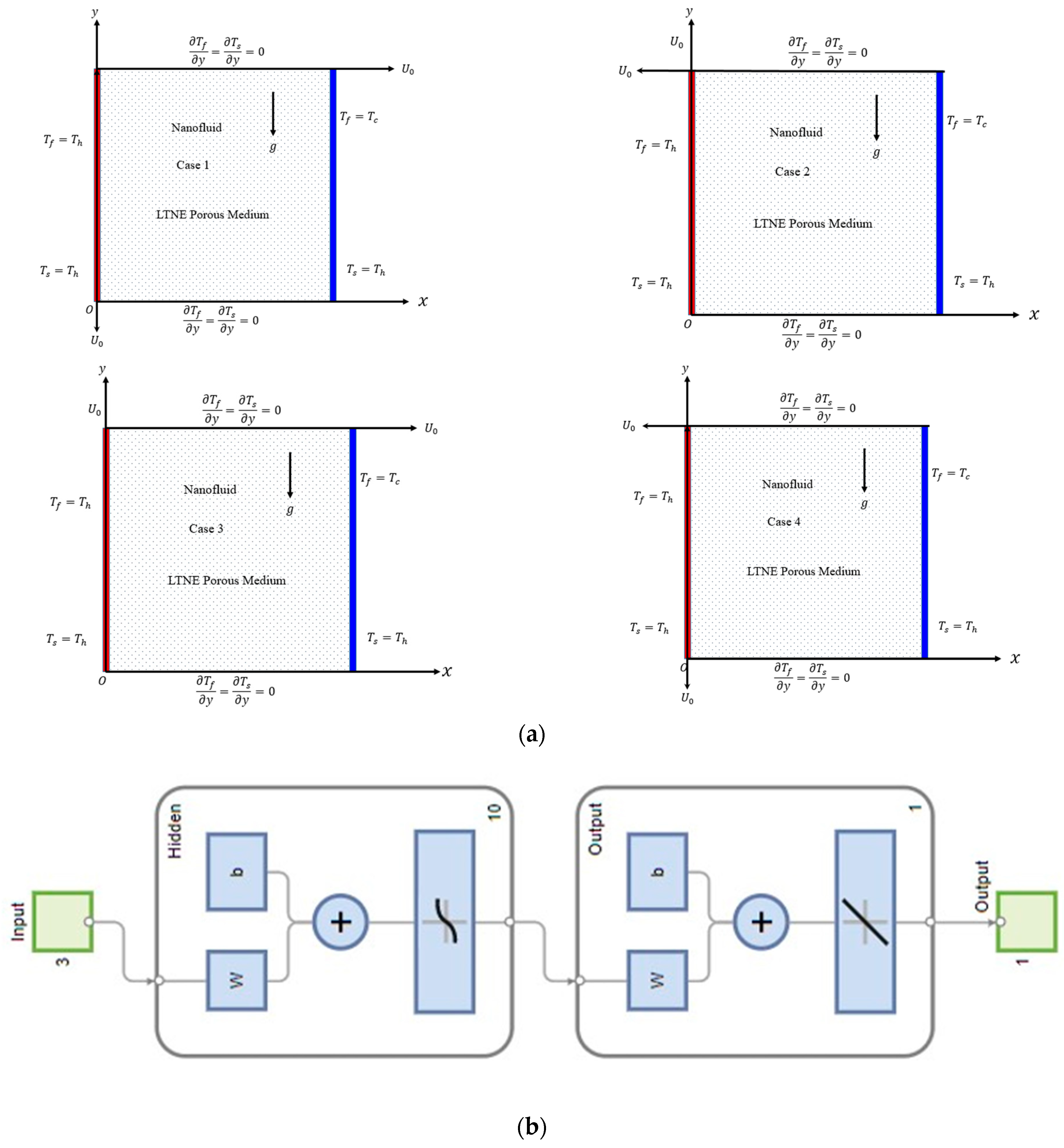
2. Formulation

The geometry of the problem and the neural network architecture for the present model are depicted in Figure 1a,b, respectively. The computational domain consists of a double-lid-driven enclosure filled with a porous medium. The left- and right-side walls of the enclosure maintain constant temperature distributions, $T_h \mathrm{and} T_c$($T_h\gg T_c$), respectively, while the upper and lower edges are thermally insulated. The top and left-side edges move with a uniform velocity, $U_0$, and several scenarios are considered based on the direction of their motion. These scenarios include the following:

• Case 1: The left-side edge moves in the negative direction of the Y-axis, and the top edge moves in the positive direction of the X-axis ($U_{Y=1}=1, V_{X=0}=-1$).
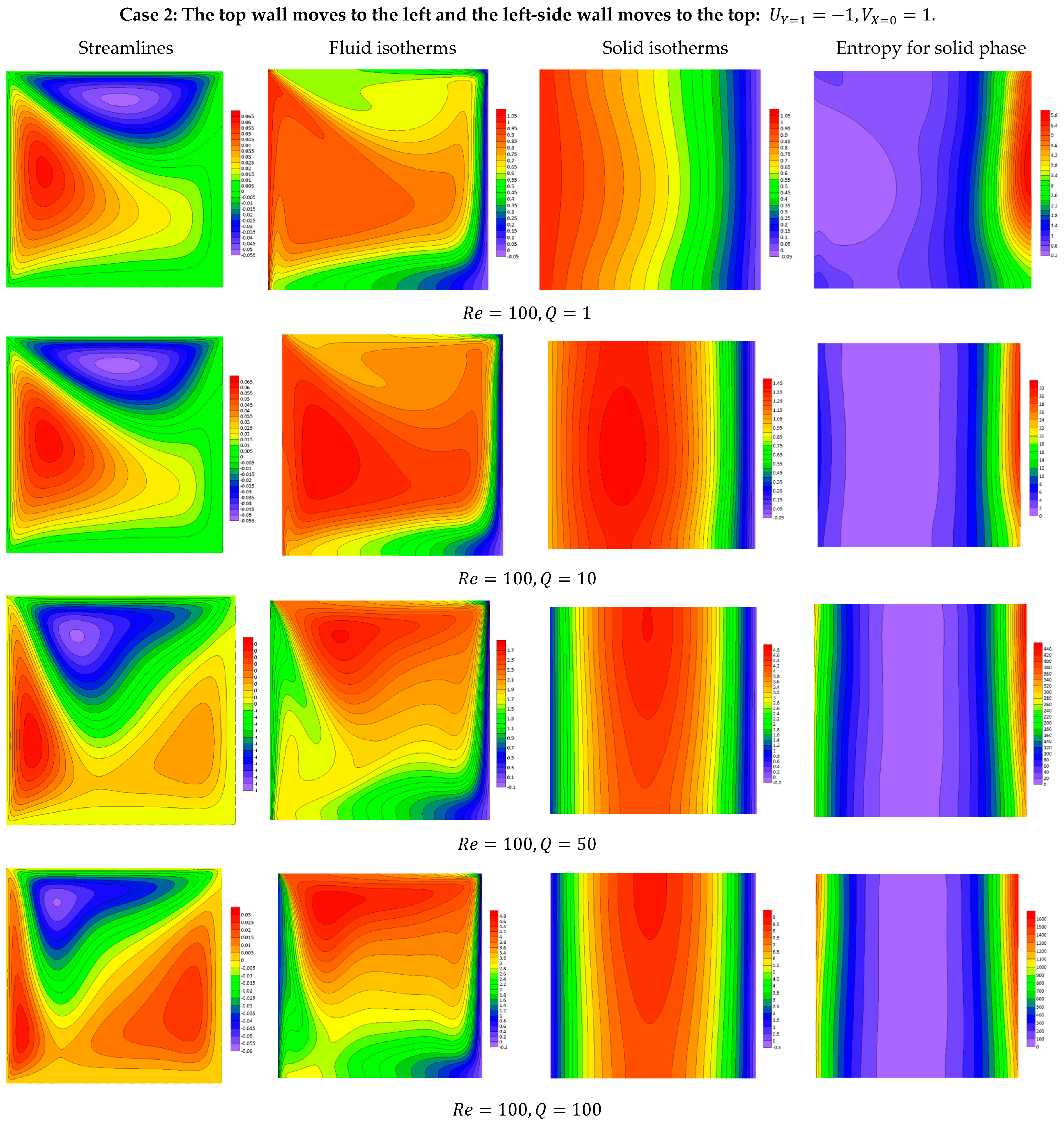
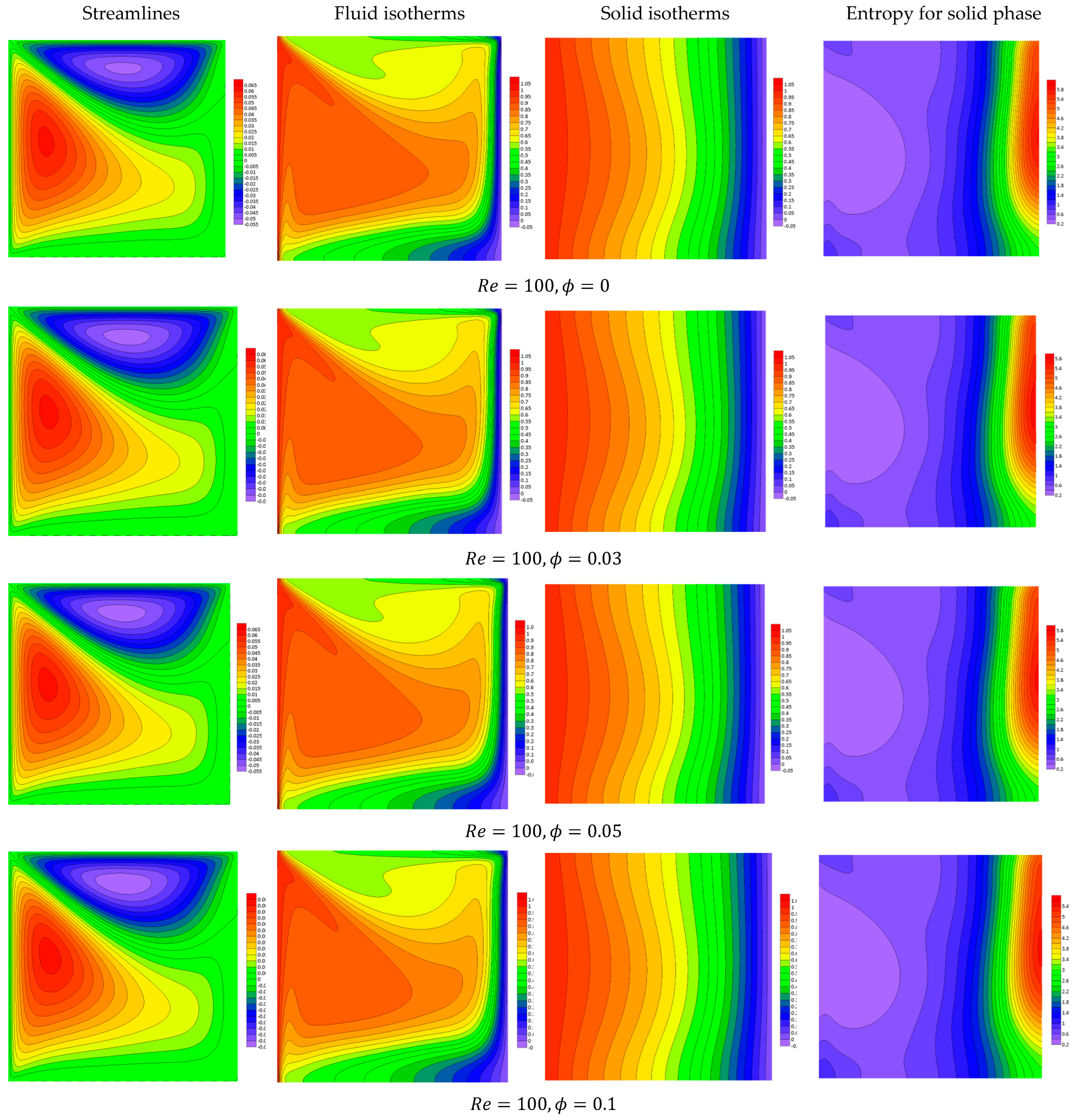
• Case 2: The left-side edge moves in the positive direction of the Y-axis, and the top edge moves in the negative direction of the X-axis ($U_{Y=1}=-1, V_{X=0}=1$).
• Case 3: Both edges move in the positive direction of their respective axes ($U_{Y=1}=1, V_{X=0}=1)$.
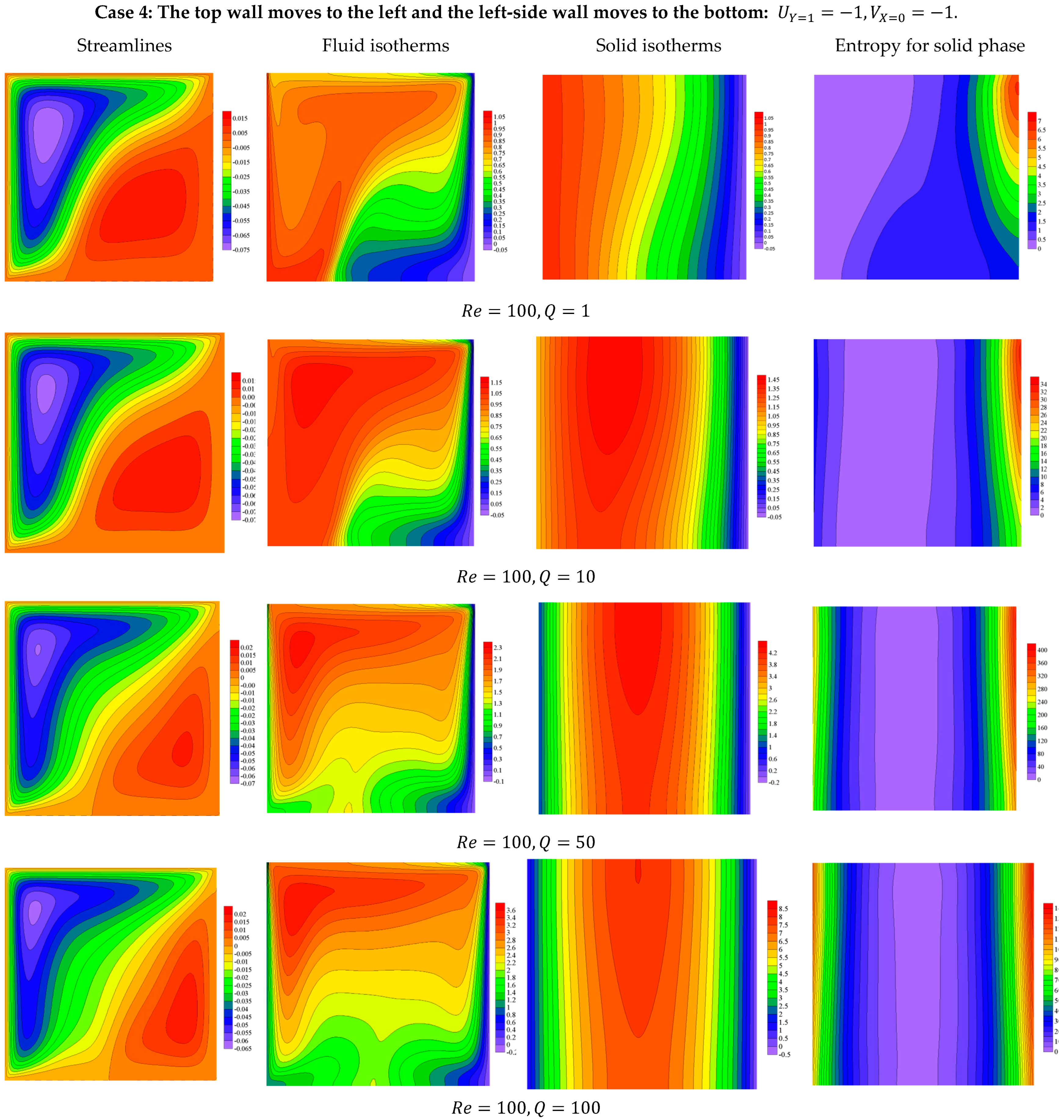
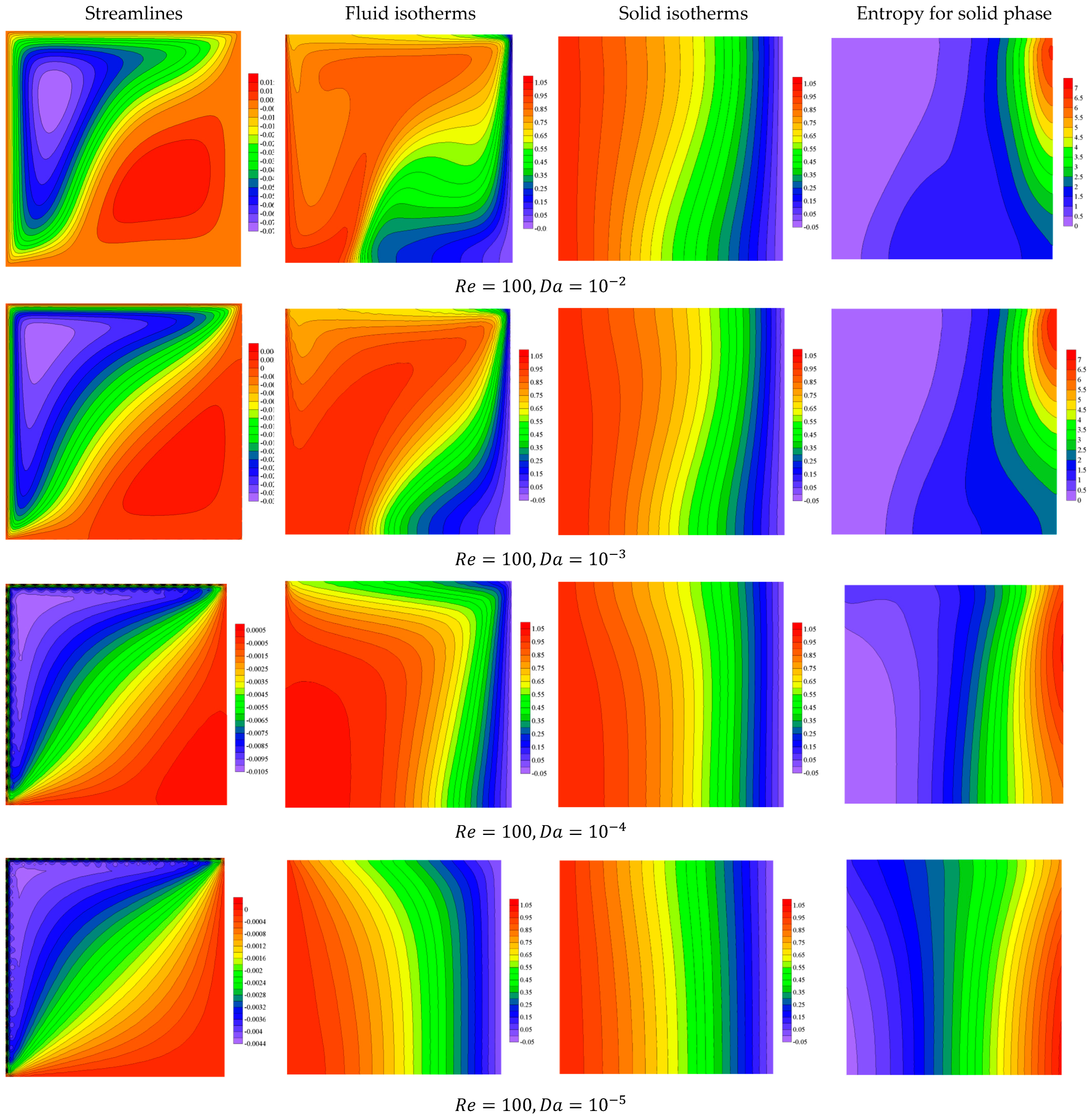
• Case 4: Both edges move in the negative direction of their respective axes ($U_{Y=1}=-1, V_{X=0}=-1)$.

Table 1. The thermophysical properties of the base fluid and nanoparticles.

Property	${\mathit{C}}_{\mathit{p}} \left(\frac{\mathbf{J}}{\mathbf{K}\mathbf{g}}\mathbf{K}\right)$	$\mathit{\rho } \left(\frac{\mathbf{K}\mathbf{g}}{{\mathbf{m}}^3}\right)$	$\mathit{k} \left(\frac{\mathbf{W}}{\mathbf{m}}\mathbf{K}\right)$	$\mathit{\beta } \left(\frac{1}{\mathbf{K}}\right)$
Water	4179	997.1	0.6	$2.1\times {10}^{-4}$
Copper	383	8954	400	$1.67\times {10}^{-5}$

summarizes the thermophysical properties of the host fluid (water) and the nanoparticles (copper) used in this study.

To accurately describe the mathematical formulation of the problem, the following hypotheses are introduced:

• The flow is laminar and steady.
• The density of the nanofluid is constant.
• Water serves as the host liquid and copper is used as the nanoparticle additive.
• The porous medium within the enclosure creates a thermal non-equilibrium (TNE) state, where a temperature difference exists between the fluid and the medium.

The equations used to test the aforementioned hypothesis are expressed as follows [28,29]:

$${\displaystyle \frac{\partial u}{\partial x}}+{\displaystyle \frac{\partial v}{\partial y}}=0$$

(1)

$${\displaystyle \frac{{\rho }_{nf}}{{\epsilon }^2}}\left[u{\displaystyle \frac{\partial u}{\partial x}}+v{\displaystyle \frac{\partial u}{\partial y}}\right]={\displaystyle \frac{{\mu }_{nf}}{\epsilon }}\left[-{\displaystyle \frac{\epsilon u}{K}}+{\displaystyle \frac{{\partial }^{2}u}{\partial x^2}}+{\displaystyle \frac{{\partial }^{2}u}{\partial y^2}}\right]-{\displaystyle \frac{\partial p}{\partial x}}$$

(2)

$${\displaystyle \frac{{\rho }_{nf}}{{\epsilon }^2}}\left[u{\displaystyle \frac{\partial v}{\partial x}}+v{\displaystyle \frac{\partial v}{\partial y}}\right]={\displaystyle \frac{{\mu }_{nf}}{\epsilon }}\left[-{\displaystyle \frac{\epsilon v}{K}}+{\displaystyle \frac{{\partial }^{2}v}{\partial x^2}}+{\displaystyle \frac{{\partial }^{2}v}{\partial y^2}}\right]-{\displaystyle \frac{\partial p}{\partial y}}+g(T_f-T_c)\left[\varphi {\rho }_{s,0}{\beta }_s+(1-\varphi ){\rho }_{f,0}{\beta }_f\right]$$

(3)

$${\left(\rho C_p\right)}_{nf}\left[u{\displaystyle \frac{\partial T_f}{\partial x}}+v{\displaystyle \frac{\partial T_f}{\partial y}}\right]=\epsilon k_{eff}\left[{\displaystyle \frac{{\partial }^2{T}_f}{\partial x^2}}+{\displaystyle \frac{{\partial }^2{T}_f}{\partial y^2}}\right]+h_{fs}\left[T_s-T_f\right]+\epsilon Q_0$$

(4)

$$\left(1-\epsilon \right)k_s\left[{\displaystyle \frac{{\partial }^2{T}_s}{\partial x^2}}+{\displaystyle \frac{{\partial }^2{T}_s}{\partial y^2}}\right]+h_{fs}\left[T_f-T_s\right]+\left(1-\epsilon \right)Q_0=0$$

(5)

$$\begin{array}{l}{s}_f={\displaystyle \frac{k_{eff}}{T_m^2}}\left[{\left({\displaystyle \frac{\partial T_f}{\partial x}}\right)}^2+{\left({\displaystyle \frac{\partial T_f}{\partial y}}\right)}^2\right]+{\displaystyle \frac{h_{fs}}{T_m^2}}{\left[T_s-T_f\right]}^2\\ +{\displaystyle \frac{{\mu }_{nf}}{T_m}}\left[{\displaystyle \frac{(u^2+v^2)}{K}}+2{\left({\displaystyle \frac{\partial u}{\partial x}}\right)}^2+2{\left({\displaystyle \frac{\partial v}{\partial y}}\right)}^2+{\left({\displaystyle \frac{\partial v}{\partial x}}+{\displaystyle \frac{\partial u}{\partial y}}\right)}^2\right]\end{array}$$

(6)

$$s_s={\displaystyle \frac{k_s}{T_m^2}}\left[{\left({\displaystyle \frac{\partial T_s}{\partial x}}\right)}^2+{\left({\displaystyle \frac{\partial T_s}{\partial y}}\right)}^2\right]+{\displaystyle \frac{h_{fs}}{T_m^2}}{\left[T_s-T_f\right]}^2$$

(7)

In the previous formulations, Equation (1) represents the continuity equation, while Equations (2) and (3) represent the momentum equations in the X- and Y-axes, respectively. The energy transport in the present system is modeled using two heat equations: one for the fluid phase (Equation (4)) and another for the solid phase (Equation (5)). Additionally, Equation (6) represents the entropy generation for the liquid phase, and Equation (7) represents the entropy generation for the medium phase. Also, $\epsilon$ is the porosity, $K$ is the permeability, $h_{fs}$ is a coefficient of the heat transfer, $Q_0$ is the heat generation, and the subscripts $f$ and $s$ refer to the liquid and medium phases. Since the water and copper nanoparticles are the components of the nanofluids, then the suitable correlations for the thermophysical properties are as follows:

$${\rho }_{nf,0}=\left(1-\varphi \right){\rho }_{f,0}+\varphi {\rho }_{s,0}$$

(8a)

$${\left(\rho C_p\right)}_{nf}=\left(1-\varphi \right){\left(\rho C_p\right)}_f+\varphi {\left(\rho C_p\right)}_s$$

(8b)

$${\displaystyle \frac{k_{eff}}{k_f}}=1+{\displaystyle \frac{k_p{A}_p}{k_f{A}_f}}+C{k}_{p}Pe{\displaystyle \frac{A_p}{k_f{A}_f}}$$

(8c)

$${\displaystyle \frac{A_p}{A_f}}={\displaystyle \frac{d_p}{d_f}}{\displaystyle \frac{\varphi }{1-\varphi }}$$

(8d)

$$Pe={\displaystyle \frac{u_p{d}_p}{{\alpha }_f}}$$

(8e)

$$u_p={\displaystyle \frac{2k_{p}T}{\pi {\mu }_f{d}_p^2}}$$

(8f)

$${\mu }_{nf}{\displaystyle \frac{{\mu }_f}{{\left(1-\varphi \right)}^{2.5}}}$$

(8g)

In the aforementioned correlations, $k_p$ is the Boltzmann parameter, $u_p$ is the Brownian motion velocity, and $d_p$ and $d_f$ are the diameters of the solid and fluid particles ($d_p=100 \mathrm{nm}, d_f=2 \AA )$.

The introduced dimensionless variables are as follows:

$${\theta }_s={\displaystyle \frac{T_s-T_c}{T_h-T_c}}, {\theta }_f={\displaystyle \frac{T_f-T_c}{T_h-T_c}}, Y={\displaystyle \frac{y}{H}}, X={\displaystyle \frac{x}{H}}, V={\displaystyle \frac{v}{U_0}}, U={\displaystyle \frac{u}{U_0}}, T_m={\displaystyle \frac{T_h+T_c}{2}}, P={\displaystyle \frac{p}{{\rho }_{nf}{U}_0^2}}$$

(9)

The following non-dimensional system is obtained based on the previous equations:

$${\displaystyle \frac{\partial U}{\partial X}}+{\displaystyle \frac{\partial V}{\partial Y}}=0$$

(10)

$${\displaystyle \frac{1}{{\epsilon }^2}}\left[U{\displaystyle \frac{\partial U}{\partial X}}+V{\displaystyle \frac{\partial U}{\partial Y}}\right]={\displaystyle \frac{1}{\epsilon }}{\displaystyle \frac{1}{Re}}{\displaystyle \frac{{\rho }_f}{{\rho }_{nf}}}{\displaystyle \frac{1}{{\left(1-\varphi \right)}^{2.5}}}\left[-{\displaystyle \frac{\epsilon U}{Da}}+{\displaystyle \frac{{\partial }^{2}U}{\partial X^2}}+{\displaystyle \frac{{\partial }^{2}U}{\partial Y^2}}\right]-{\displaystyle \frac{\partial P}{\partial X}}$$

(11)

$${\displaystyle \frac{1}{{\epsilon }^2}}\left[U{\displaystyle \frac{\partial V}{\partial X}}+V{\displaystyle \frac{\partial V}{\partial Y}}\right]={\displaystyle \frac{1}{\epsilon }}{\displaystyle \frac{1}{Re}}{\displaystyle \frac{{\rho }_f}{{\rho }_{nf}}}{\displaystyle \frac{1}{{\left(1-\varphi \right)}^{2.5}}}\left[-{\displaystyle \frac{\epsilon V}{Da}}+{\displaystyle \frac{{\partial }^{2}V}{\partial X^2}}+{\displaystyle \frac{{\partial }^{2}V}{\partial Y^2}}\right]-{\displaystyle \frac{\partial P}{\partial Y}}+{\displaystyle \frac{Ra}{{Re}^{2}Pr}}{\displaystyle \frac{{\rho }_{f,0}}{{\rho }_{nf,0}}}\left(1-\varphi +\varphi {\displaystyle \frac{{\rho }_s{\beta }_s}{{\rho }_f{\beta }_f}}\right){\theta }_f$$

(12)

$$U{\displaystyle \frac{\partial {\theta }_f}{\partial X}}+V{\displaystyle \frac{\partial {\theta }_f}{\partial Y}}=\epsilon {\displaystyle \frac{k_{nf}}{k_f}}{\displaystyle \frac{{\left(\rho C_p\right)}_f}{{\left(\rho C_p\right)}_{nf}}}{\displaystyle \frac{1}{Re}}{\displaystyle \frac{1}{Pr}}\left[{\displaystyle \frac{{\partial }^2{\theta }_f}{\partial X^2}}+{\displaystyle \frac{{\partial }^2{\theta }_f}{\partial Y^2}}\right]+{\displaystyle \frac{Hs}{Re Pr}}{\displaystyle \frac{{\left(\rho C_p\right)}_f}{{\left(\rho C_p\right)}_{nf}}}\left[{\theta }_s-{\theta }_f\right]+{\displaystyle \frac{\epsilon }{Re Pr}}{\displaystyle \frac{{\left(\rho C_p\right)}_f}{{\left(\rho C_p\right)}_{nf}}}Q$$

(13)

$$\left[{\displaystyle \frac{{\partial }^2{\theta }_s}{\partial X^2}}+{\displaystyle \frac{{\partial }^2{\theta }_s}{\partial Y^2}}\right]+{\displaystyle \frac{Hs}{1-\epsilon }}{k}_{ratio}\left[{\theta }_f-{\theta }_s\right]+k_{ratio}Q=0$$

(14)

The subjected boundary conditions are also transformed to the dimensionless form as follows:

Through the left-side edge:

$$U=0, V=\pm 1, {\theta }_f={\theta }_s=1$$

(15a)

Through the right-side edge:

$$U=0, V=0, {\theta }_f={\theta }_s=0$$

(15b)

Through the upper edge:

$$V=0,U=\pm 1, {\displaystyle \frac{\partial {\theta }_f}{\partial Y}}={\displaystyle \frac{\partial {\theta }_s}{\partial Y}}=0$$

(15c)

Through the lower edge:

$$V=0,U=0, {\displaystyle \frac{\partial {\theta }_f}{\partial Y}}={\displaystyle \frac{\partial {\theta }_s}{\partial Y}}=0$$

(15d)

Also, the dimensionless entropy equations are given as follows:

$$S_F=s_f.{\displaystyle \frac{T_m^2{H}^2}{k_f{(∆T)}^2}}={\displaystyle \frac{k_{nf}}{k_f}}\left[{\left({\displaystyle \frac{\partial {\theta }_f}{\partial X}}\right)}^2+{\left({\displaystyle \frac{\partial {\theta }_f}{\partial Y}}\right)}^2\right]+Hs{\left[{\theta }_s-{\theta }_f\right]}^2+{\lambda }_1{\displaystyle \frac{{\mu }_{nf}}{{\mu }_f}}\left[{\displaystyle \frac{(U+V^2)}{Da}}+2{\left({\displaystyle \frac{\partial U}{\partial X}}\right)}^2+2{\left({\displaystyle \frac{\partial V}{\partial Y}}\right)}^2+{\left({\displaystyle \frac{\partial V}{\partial X}}+{\displaystyle \frac{\partial U}{\partial Y}}\right)}^2\right]$$

(16)

$$S_S=s_s.{\displaystyle \frac{T_m^2{H}^2}{k_f{(∆T)}^2}}={\displaystyle \frac{1}{k_{ratio}}}\left[{\left({\displaystyle \frac{\partial {\theta }_s}{\partial X}}\right)}^2+{\left({\displaystyle \frac{\partial {\theta }_s}{\partial Y}}\right)}^2\right]+Hs{\left[{\theta }_s-{\theta }_f\right]}^2$$

(17)

The previous equations contain important factors, which are defined as follows:

• $Re={\displaystyle \frac{H{U}_0}{{\nu }_f}}$ is the Reynolds coefficient.
• $Pr={\displaystyle \frac{{\nu }_f}{{\alpha }_f}}$ is the Prandtl coefficient.
• $Hs={\displaystyle \frac{H^2{h}_{fs}}{k_f}}$ is the heat transport parameter.
• $Q={\displaystyle \frac{Q_{0H^2}}{∆T{k}_f}}$ is the heat generation parameter.
• $k_{ratio}={\displaystyle \frac{k_f}{k_s}}$ is the temperature conductivity ratio.

During these investigations, there are two rates of heat transfer, namely, for the solid phase and for the liquid phase. These quantities are given as follows:

$${Nu}_f\left(Y\right)=-{\displaystyle \frac{k_{nf}}{k_f}}{{\displaystyle \frac{\partial {\theta }_f}{\partial X}}|}_{X=0, 1}$$

(18)

$${Nu}_s\left(Y\right)=-{{\displaystyle \frac{\partial {\theta }_s}{\partial X}}|}_{X=0, 1}$$

(19)

$${Nu}_{mf}={\int }_0^1{Nu}_f\left(Y\right)dY$$

(20)

$${Nu}_{ms}={\int }_0^1{Nu}_s\left(Y\right)dY$$

(21)

3. Numerical Solution

The governing equations for the problem are solved numerically using the finite volume method (FVM), which ensures the conservation of mass, momentum, and energy within each control volume. The computational domain is discretized into a structured Cartesian mesh, splitting the domain into a large number of small control volumes $\Omega$. In these treatments, Equations (10)–(12) are discretized, including advection and diffusive terms, as well as source terms as follows:

$${\oint }_S\mathit{V}·\mathit{n} dS=0$$

(22)

$$\begin{gathered} {\oint }_{S}P·ndS+{\displaystyle \frac{1}{{\epsilon }^2}}{\oint }_S\left(\mathit{V}\mathit{V}\right)·\mathit{n}dS-{\displaystyle \frac{1}{\epsilon }}{\displaystyle \frac{1}{Re}}{\displaystyle \frac{{\rho }_f}{{\rho }_{nf}}}{\displaystyle \frac{1}{{\left(1-\varphi \right)}^{2.5}}}{\oint }_S\left(\nabla V\right)·ndS+{\displaystyle \frac{1}{Re}}{\displaystyle \frac{{\rho }_f}{{\rho }_{nf}}}{\displaystyle \frac{1}{{\left(1-\varphi \right)}^{2.5}}}{\int }_{\Omega }\mathit{V}d\Omega +S_{\theta }{\int }_{\Omega }\mathit{V}d\Omega \\ -\chi {\displaystyle \frac{Ra}{{Re}^{2}Pr}}{\displaystyle \frac{{\rho }_{f,0}}{{\rho }_{nf,0}}}\left(1-\varphi +\varphi {\displaystyle \frac{{\rho }_s{\beta }_s}{{\rho }_f{\beta }_f}}\right){\int }_{\Omega }\theta d\Omega =0 \end{gathered}$$

(23)

where $\mathit{V}$ refers to the velocity vector and $\chi$ is a parameter, where $\chi =0$ for $U$-equations and $\chi =1$ for $V$-equations, with convergence conditions of the order of ${10}^{-6}$.

The resultant system of equations is iteratively solved using the Alternating Direction Implicit (ADI) method, which enhances computational efficiency and stability. The SIMPLER algorithm is employed to couple velocity and pressure corrections, iteratively solving the momentum and continuity equations. The boundary conditions include constant temperature distributions (${\mathit{T}}_{\mathit{h}} \mathrm{a}\mathrm{n}\mathrm{d} {\mathit{T}}_{\mathit{c}})$ on the left- and right-side walls, insulated conditions on the upper and lower edges, and uniform velocity ${\mathit{U}}_0$ on the moving walls.

Table 2. The values of the main Nusselt coefficients in the absence of LTNEM and $Da\to \infty$, $Gr=100, \varphi =0$.

$$\mathit{R}\mathit{e}$$	100	400	1000
Iwatsu et al. [30]	1.94	3.84	6.33
Khanafer and Chamkha [31]	2.01	3.91	6.33
Present study	1.93	3.91	6.31

presents the accuracy test of the proposed technique, where comparisons with previously published data are performed under specific conditions: the absence of local thermal non-equilibrium (LTNEM), $\mathit{D}\mathit{a}\to \mathit{\infty }$, $\mathit{G}\mathit{r}=100, \mathrm{a}\mathrm{n}\mathrm{d} \mathit{\varphi }=0$. These results demonstrate the reliability of the method by showing excellent agreement with prior studies.

The solution procedure involves initializing all variables, iteratively solving the discretized equations using the ADI method, and updating the field values until residuals are below a specified tolerance (${10}^{-6}$). This approach ensures accurate simulation of the flow and thermal behavior within the enclosure.

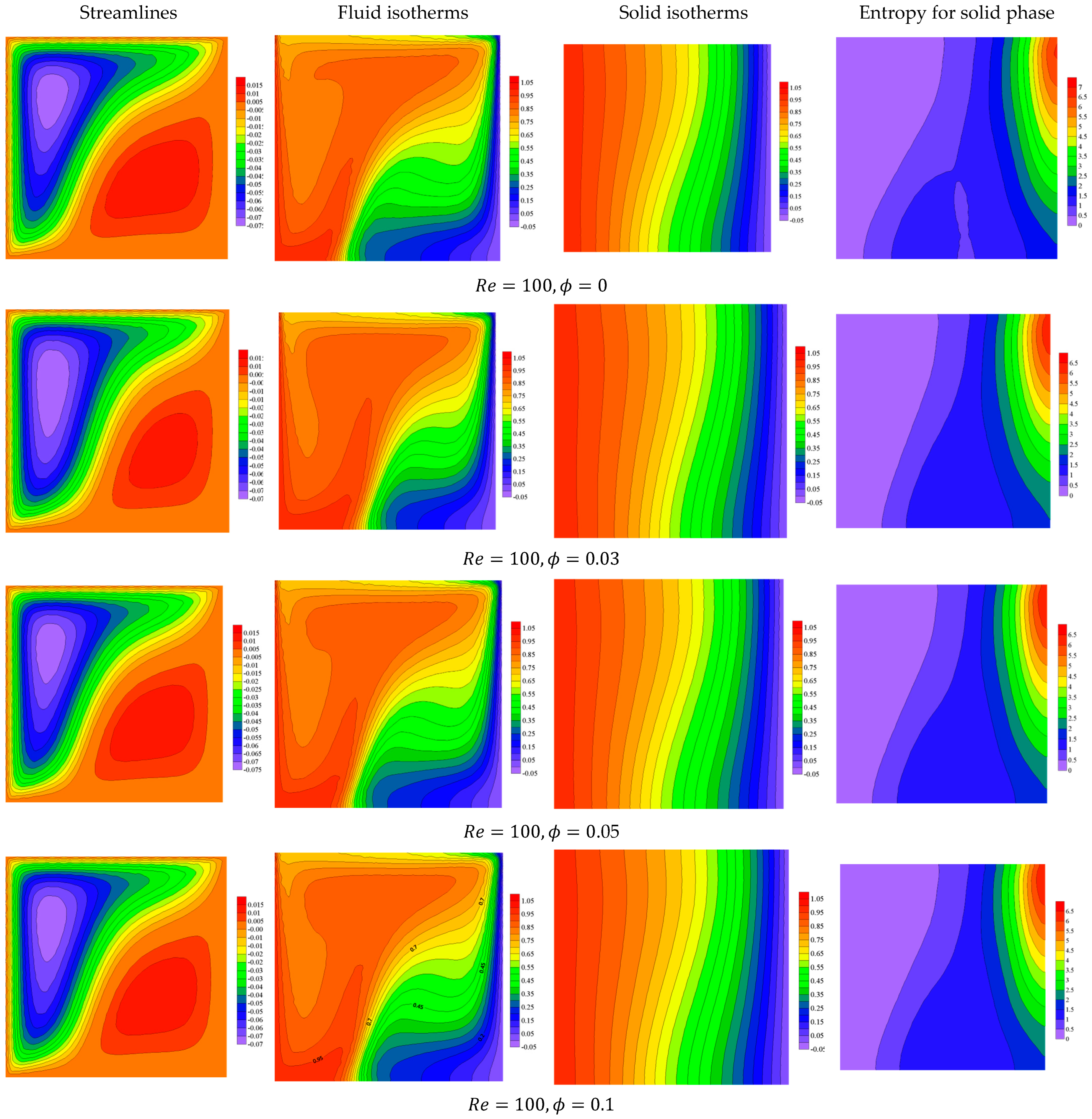
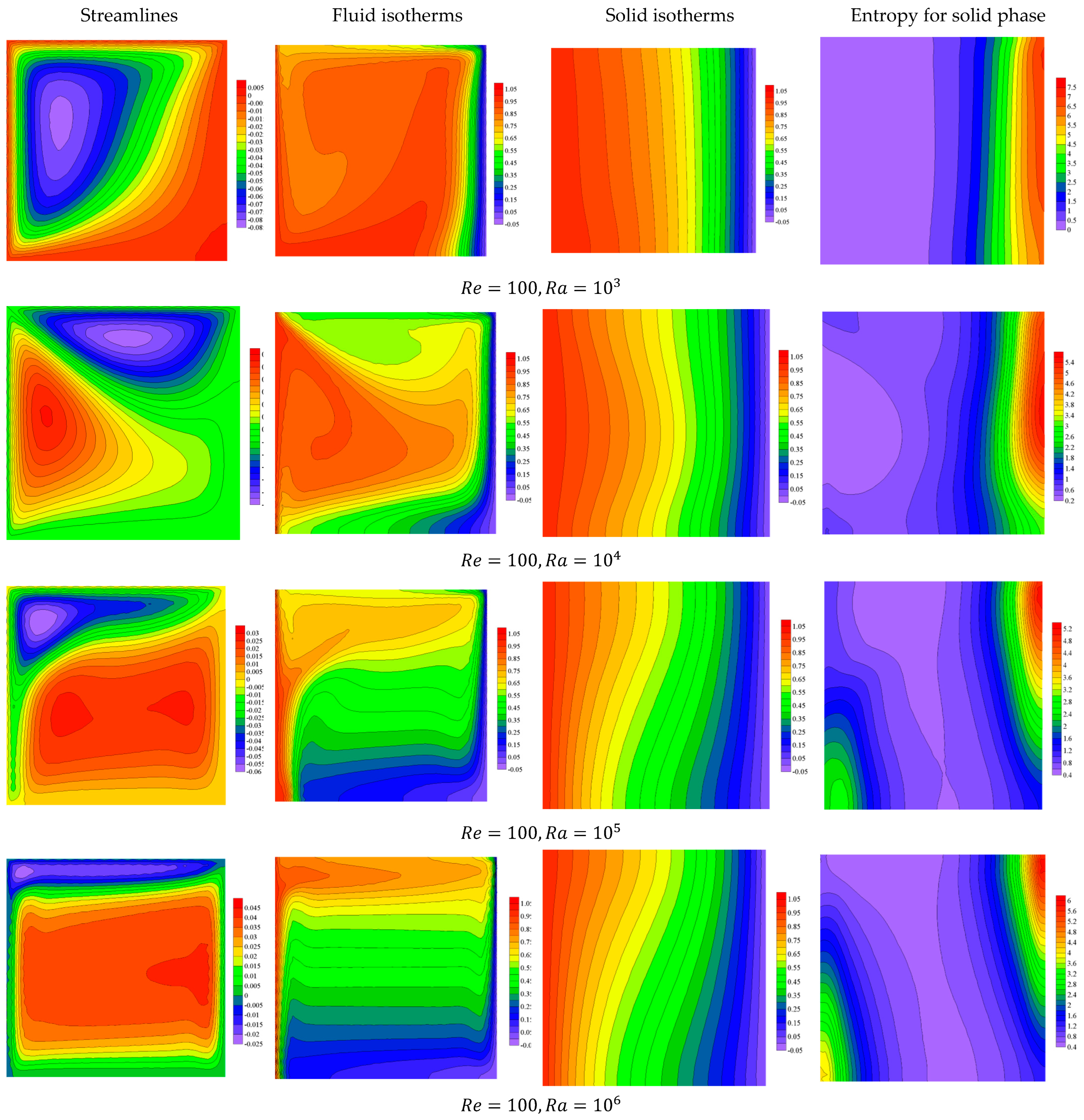
4. Results and Discussion

This division presents a discussion of the given outcomes. In this investigation, the results are presented for four cases, and the roles of the aforementioned parameters—the heat generation parameter $Q(1\le Q\le 100)$; the Darcy number $Da$ (${10}^{-5}\le Da\le {10}^{-2})$; the nanoparticle volume fraction $\varphi \left(0\%\le \varphi \le 5\%\right);$ the Rayleigh number $Ra ({10}^3\le Ra\le {10}^5)$ for the streamlines, fluid isotherms, and solid isotherms; the entropy for the solid phase; and the local Nusselt numbers for the liquid and medium phases—are studied.

Figure 2, Figure 3, Figure 4 and Figure 5 show features of the streamlines, fluid isotherms, solid isotherms, and the entropy for the solid phase for Case 1, where $U_{Y=1}=1, V_{X=0}=-1$, against the variations in $Q, Da, \varphi$, and $Ra$. These illustrations are performed as a referenced case, where $Re=100, Da=0.01, Q=1, H=1, \varphi =1\%, Ra={10}^3.$ It is remarkable that the flow shows a major anti-clockwise eddy due to the top wall movement and a minor clockwise eddy due to the left-side wall movement. Also, the convection mode is dominant on the fluid isotherms, while the conduction mode is dominant on the solid isotherms. Furthermore, the solid phase irreversibility is seen within the entire domain, but the isotherms gather near the cold wall (right-side edge of the domain). The results highlight the complex flow and thermal behavior in the system. The dominant anti-clockwise eddy driven by the top wall movement reflects the primary circulation, while a minor clockwise eddy near the left-side wall indicates localized recirculation. In the fluid region, heat transfer is primarily governed by convection, as indicated by the fluid isotherms, whereas in the solid region, conduction dominates due to the absence of fluid motion. The solid phase exhibits entropy generation across the domain due to temperature gradients, with irreversibility clustering near the cold wall (right-side edge), signifying high thermal gradients and localized energy losses. These findings provide valuable insights into optimizing heat transfer and minimizing entropy generation in similar systems. The findings also disclose that the rise in the heat generation coefficient, $Q$, causes an enhancement in the activity of the motion due to the improvement in the temperature differences. A good isotherms domain is obtained as $Q$ increases due to the additional heat generation within the domain. Further, the irreversibility due to the solid phase rises as $Q$ increases due to the rise in the temperature gradients. In the same context, the variation in the Darcy number values (from ${10}^{-2}$ to ${10}^{-5})$ causes the flow to diminish, and the forced convection becomes dominant. Also, both the fluid and medium isotherms and solid phase entropy reveal that the conduction case controls at the lower values of $Da$ compared to the convection mode. All these features are due to the decrease in the medium permeability as $Da$ is decreased. Regarding the variation in $\varphi$, the illustrations show that the flow becomes more viscous due to the increase in $\varphi$ and hence the mixed mode diminishes. Regarding the variations in the Rayleigh coefficient, the figures illustrate that the low values of $Ra$ indicate that the forced mode controls the flow domain, while the increasing value of Ra indicates that the buoyancy-driven flow is dominant.

For Case 2, where the top wall moves in the inverse direction of the $X$-axis and the left-side wall moves in the positive direction of the $Y$-axis ($U_{Y=1}=-1, V_{X=0}=1)$, the features of the streamlines and fluid/solid isotherms and the entropy property for the medium phase under the impacts of the governing parameters $Q, Da, \varphi ,$ and $Ra$ are depicted in Figure 6, Figure 7, Figure 8 and Figure 9. Here, the flow structures differ from the previous case, where the major anticlockwise eddy is seen near the left-side edge and the minor clockwise eddy is noted close to the top edge. Also, the most heated zone occurs near the left-side boundary, indicating a good convection area, while the irreversibility of the solid phase occurs near the right-side edge. Like the previous case, the increase in either $Q$ or the Rayleigh number $Ra$ causes an enhancement in the temperature difference, which results in an improvement in buoyancy force and natural convection mode. When both the heat generation parameter and the Rayleigh number are high, the following results are observed:

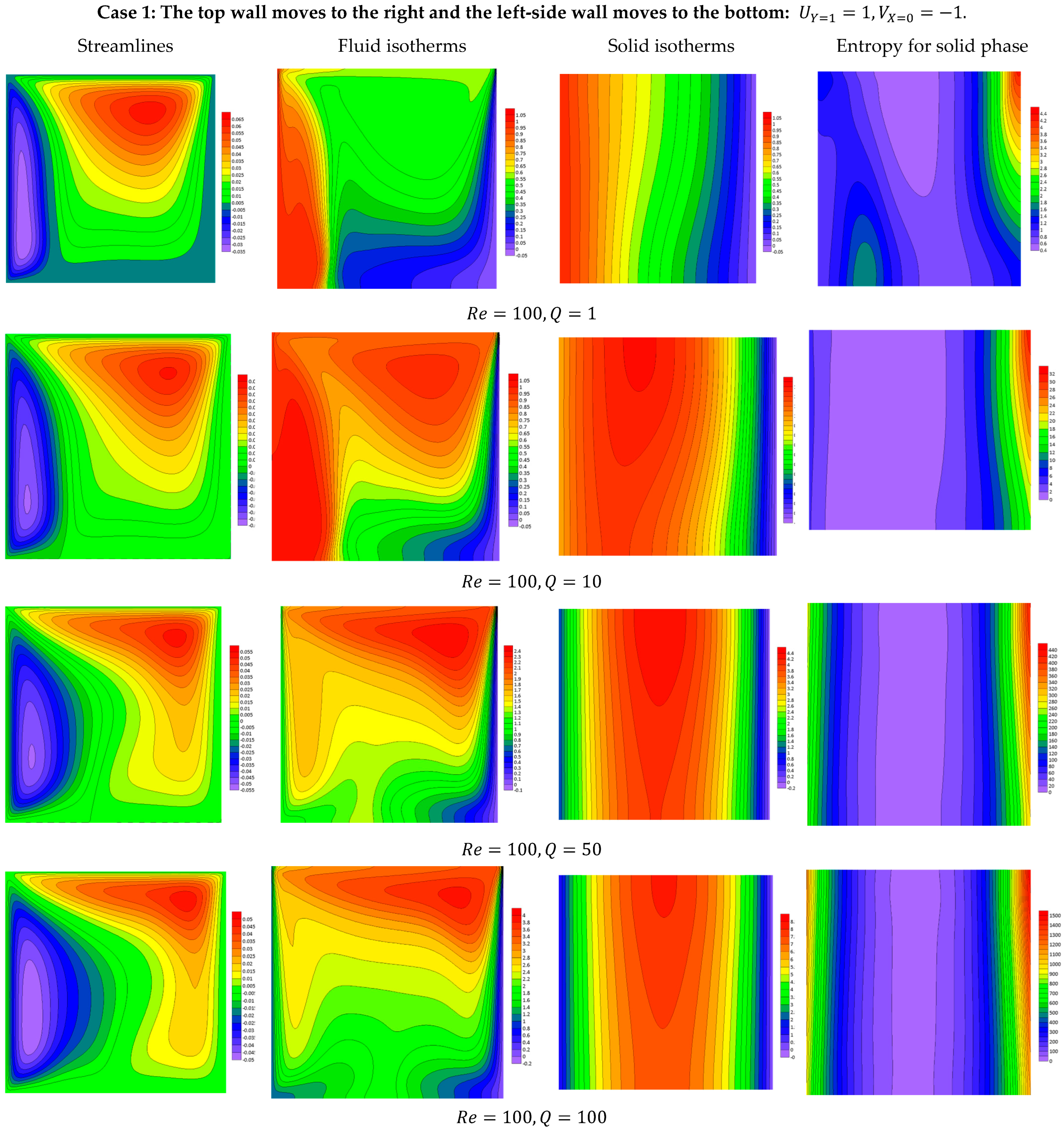
• The heat generation increases the driving temperature difference.
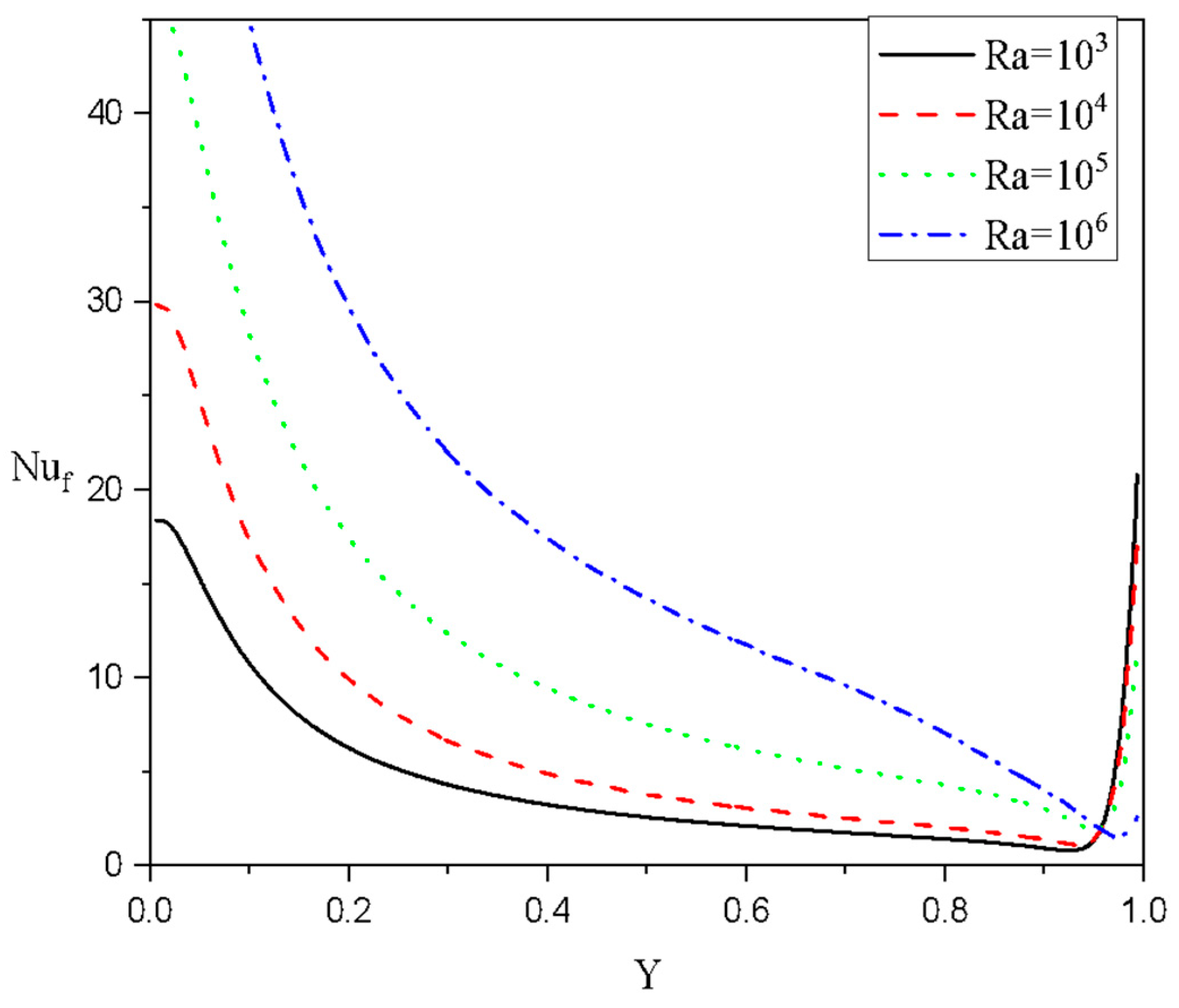
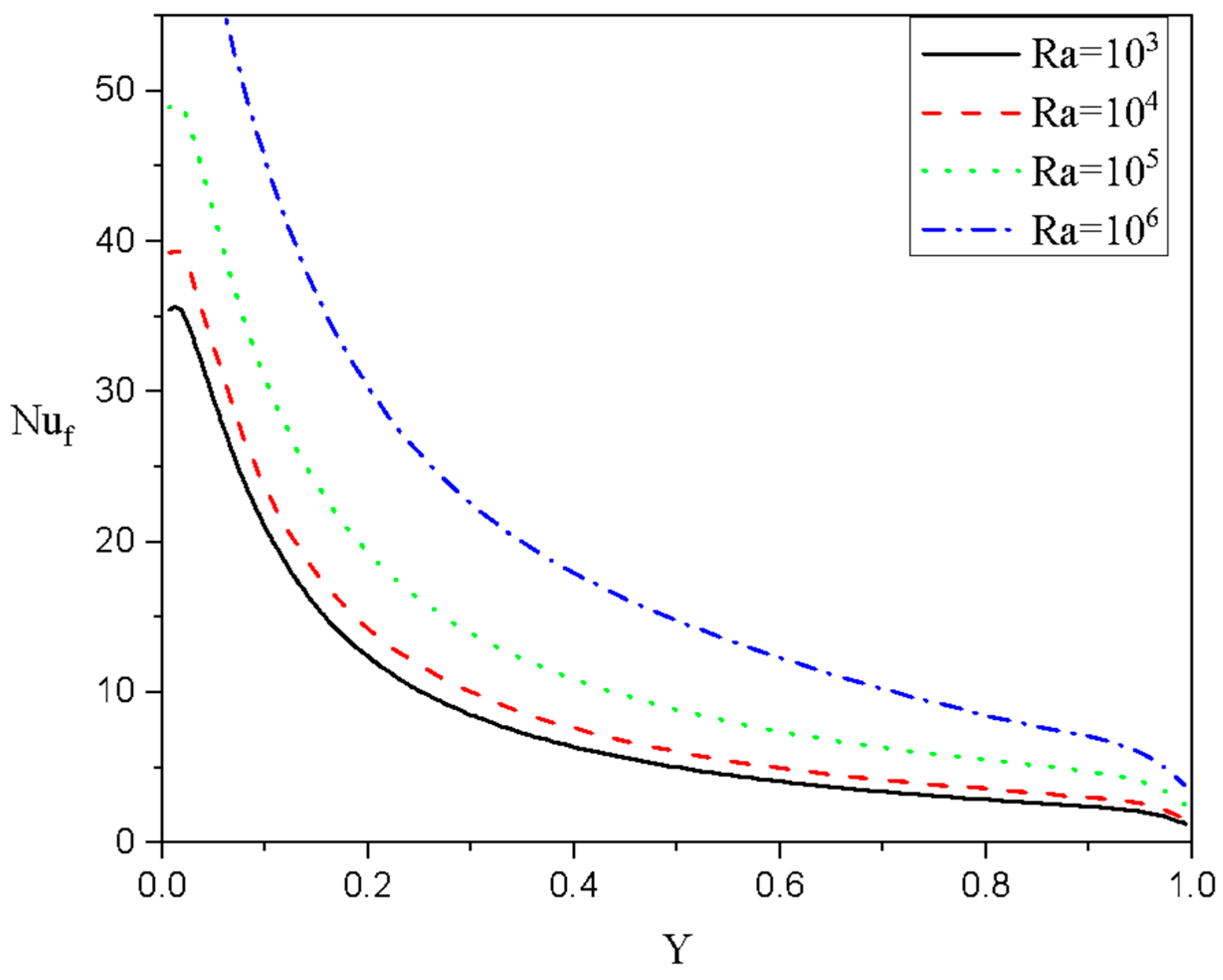
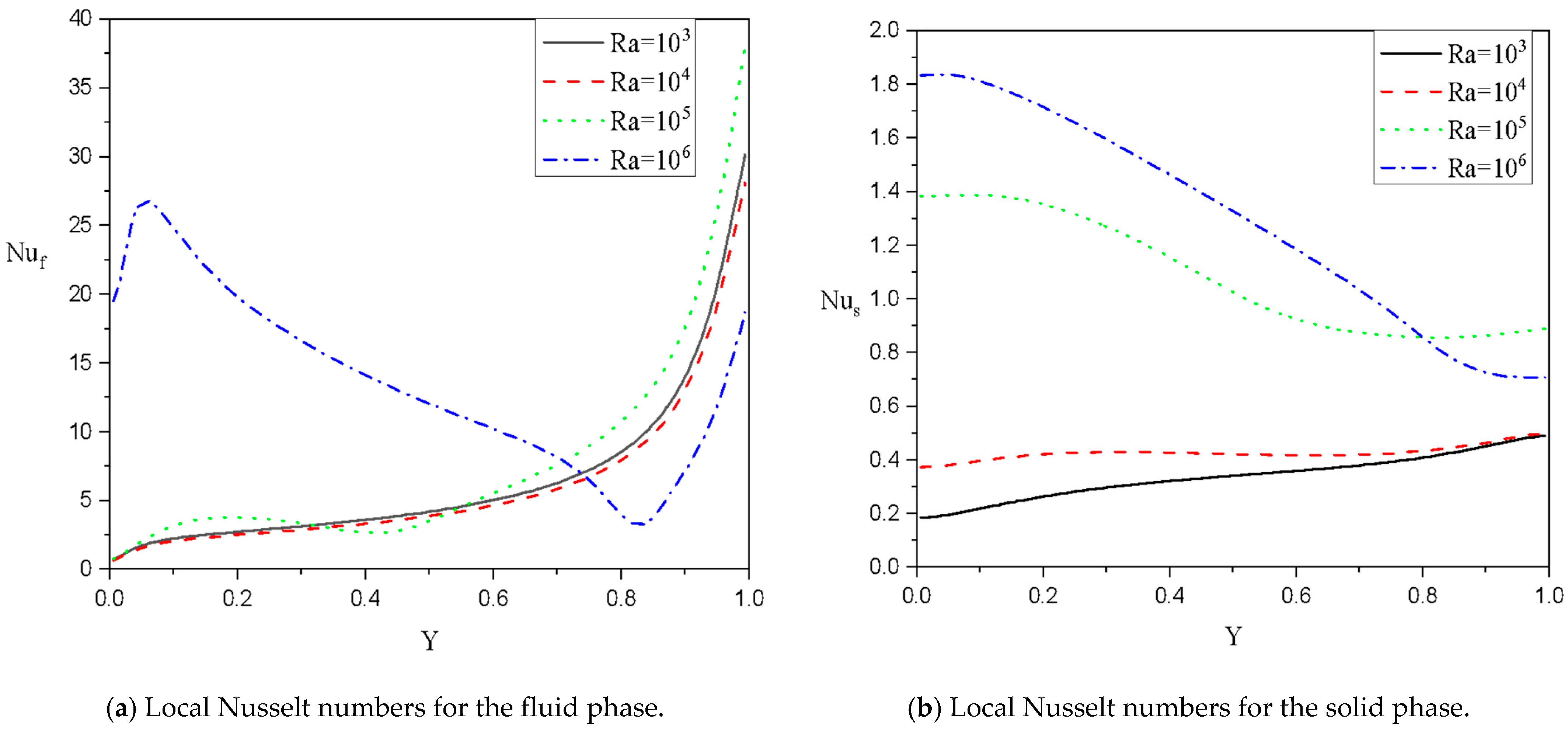
• The Rayleigh number amplifies the effect of buoyancy forces, resulting in a stronger, more dynamic convective flow.
• The system transitions from conduction-dominated to convection-dominated heat transfer, making the convective mode the primary mechanism of energy transport.

Also, the permeability of the medium diminishes as $Da$ increases and hence the flow is slowed down. Small variations in the flow and temperature features are seen as $\varphi$ increases due to the rise in the basic viscosity of the liquid.

Figure 10, Figure 11, Figure 12 and Figure 13 display the thermal fields and flow structures for variations in the governing parameter, i.e., heat generation parameter $Q$, Darcy number $Da$, nanoparticle volume fraction $\varphi$, and the Rayleigh number $Ra$ at $Re=100$. Here, the top and left-side walls are moving in the negative directions of the $X$- and $Y$-axes, respectively, and this case is termed Case 4. Due to the directions of the movements of the edges, a major forced eddy is formulated within the domain while a small anticlockwise eddy is noted near the bottom right-side corner of the chamber. Also, the temperature features are affected by the directions of the movements. Here, a large heated area is noted near the top left-side corner of the domain while a small cold zone is observed near the bottom right-side corner. The illustrations also show that the growth in heat generation coefficient enhances the natural convection and the irreversibility of the solid phase becomes higher. The flow structures are strongly affected by variations in $Da$. Here, the convection cell disappears and the forced flow controlling the domain as $Da$ decreases due to the obstruction of the medium elements. Additionally, the lower values of $Da$ cause a dominance of the conduction on the isotherms and the irreversibility of the medium phase distributes within the whole cavity. From the physical view, the behavior associated with a lower Darcy number (Da) reflects the impact of reduced permeability on heat and entropy transfer within the medium. A lower Da indicates that the porous medium significantly restricts fluid flow, effectively suppressing convection and making conduction the dominant mode of heat transfer. This results in more evenly spaced isotherms, which is characteristic of conduction-dominated heat transfer. Additionally, the irreversibility in the medium phase becomes more uniformly distributed throughout the cavity due to the limited fluid motion, as temperature gradients are the primary contributors to entropy generation in the absence of strong convective effects. This behavior underscores the critical role of permeability in influencing heat and energy dissipation mechanisms in a porous system. Interesting features for the flow and isotherms are seen within the chamber as the Rayleigh coefficient is varied. Here, the higher values of $Ra$ cause the convection cell to become enlarged and occupy the entire domain.

Figure 14 shows the local Nusselt values for the fluid phase along the active edge for several values of $Da$ at $Q=1, Hs=1, \varphi =1\%, Ra={10}^3, \lambda =0.0001$, and Case 1: $U_{Y=1}=1, V_{X=0}=-1.$ We can note that the lower values of $Da$ cause a gradual increase in ${Nu}_f$ due to the increase in the gradients of the fluid temperature. For the same case (Case 1: $U_{Y=1}=1, V_{X=0}=-1$), profiles of the fluid–Nusselt coefficient for several values of $Ra$ at $Re=100$ and $Da=0.01$ are presented in Figure 15. It is observed that ${Nu}_f$ increases with $Ra$ due to the growing convective situation while the higher values of $Ra$ ($Ra={10}^6)$ cause an extra increase, and thus the ${Nu}_f$ profile is reversed.

For Case 2: $U_{Y=1}=-1, V_{X=0}=1$, the behaviors of the local Nusselt numbers for the liquid ${Nu}_f$ and medium ${Nu}_s$ phases under the impact of the Darcy coefficient $Da$ are depicted in Figure 16. For these conditions, the maximum values of ${Nu}_f$ occur near the bottom wall while ${Nu}_s$ has a minimum value that occurs in the middle of the lower edge. We can note that the increase in $Da$ causes an improvement in gradients of the fluid temperature and hence ${Nu}_f$ is augmented. Also, near the bottom wall, ${Nu}_s$ enhances as $Da$ grows due to the dissipation effects. In a related context, Figure 17 shows the local Nusselt quantity along the heated wall for the fluid phase for several values of $Ra$ at $\varphi =1\%, Hs=1, Da=0.01, Q=1, \lambda =0.0001$ and Case 2: $U_{Y=1}=-1, V_{X=0}=1.$ It is noticeable that the temperature differences are improved as $Ra$ is altered, and hence the rate of heat transport is augmented.

Figure 18 displays the local Nusselt values along the heated boundary for the liquid and medium phases for various values of $Da$ at $Q=1, Hs=1, \varphi =1\%, Ra={10}^3, \lambda =0.0001$ and Case 3: $U_{Y=1}=1, V_{X=0}=1$. It is noted that ${Nu}_f$ gradually increases as $Da$ is enhanced, while only the lower part of the left-side edge ${Nu}_s$ is enhanced as Da is altered. By comparing ${Nu}_f$ and ${Nu}_s$ in this case and in the previous case ($U_{Y=1}=-1, V_{X=0}=1)$, we can note that the rate of the heat transport is higher in Case 3, where $U_{Y=1}=1, V_{X=0}=1$. Figure 19 shows the local Nusselt quantity in the heated part of the system for the fluid phase for several values of $Ra$ at $\varphi =1\%, Hs=1, Ra={10}^3, Q=1, \lambda =0.0001$ and Case 3: $U_{Y=1}=1, V_{X=0}=1.$ The figure shows a good enhancement in ${Nu}_f$ as $Ra$ is altered because of the thermal boundary layer’s thickness.

For Case 4, where $U_{Y=1}=-1, V_{X=0}=-1$, the impacts of $Da$ and $Ra$ on the Nusselt numbers for the liquid and medium phases ${(Nu}_f$, ${Nu}_s)$ are studied using Figure 20 and Figure 21. The illustrations revealed that both ${Nu}_f$ and ${Nu}_s$ take higher features as either $Da$ or $Ra$ increase.

These results provide valuable contributions to understanding the interplay between thermal and fluid dynamics in porous media. However, the applications of these findings could be further emphasized, particularly in the context of real-world engineering applications. For instance, discussing how the observed trends in entropy generation and heat transfer efficiency might inform the design of advanced thermal management systems, energy-efficient devices, or porous media heat exchangers would enhance this study’s applicability and relevance to industrial contexts.

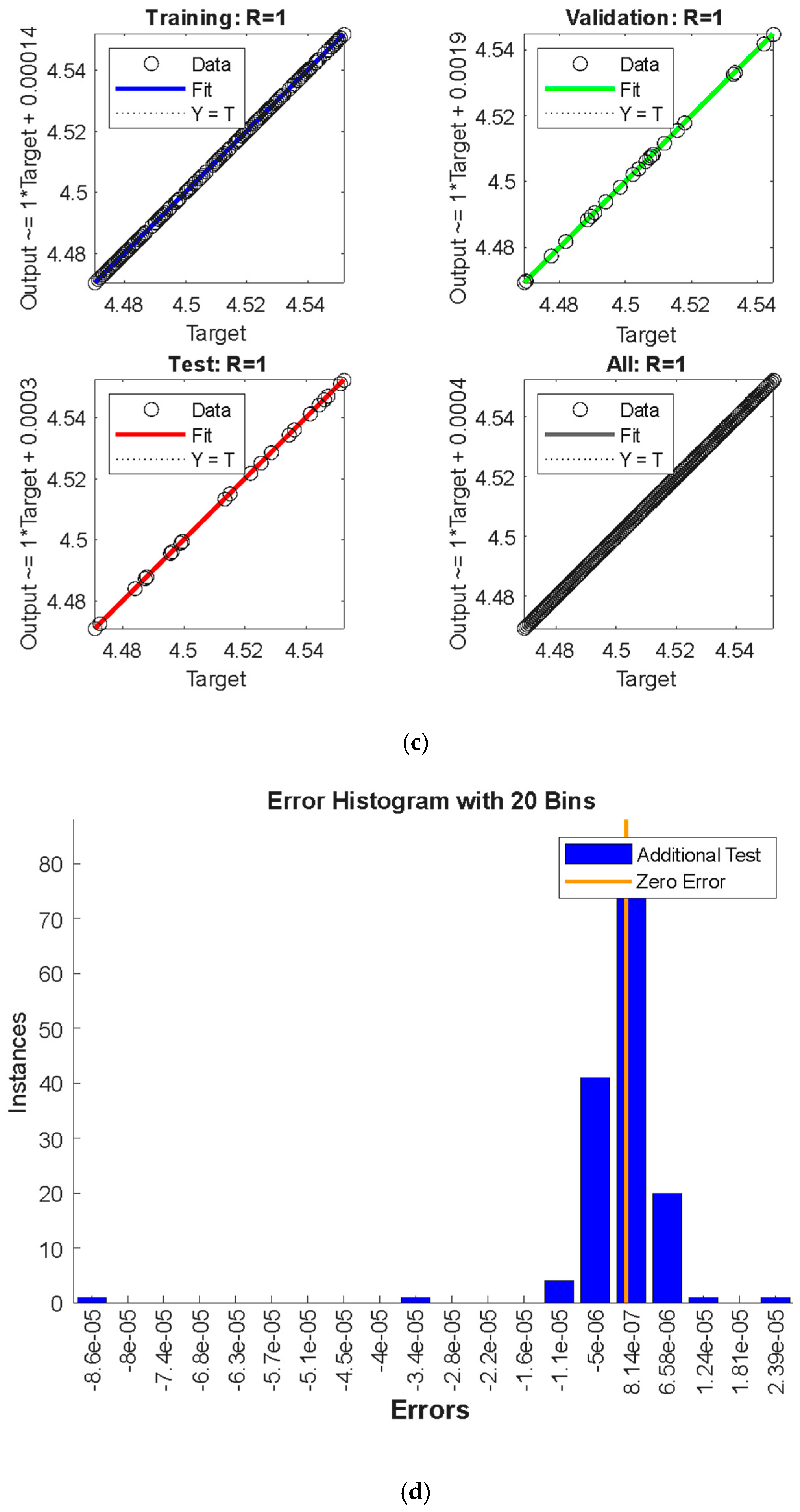
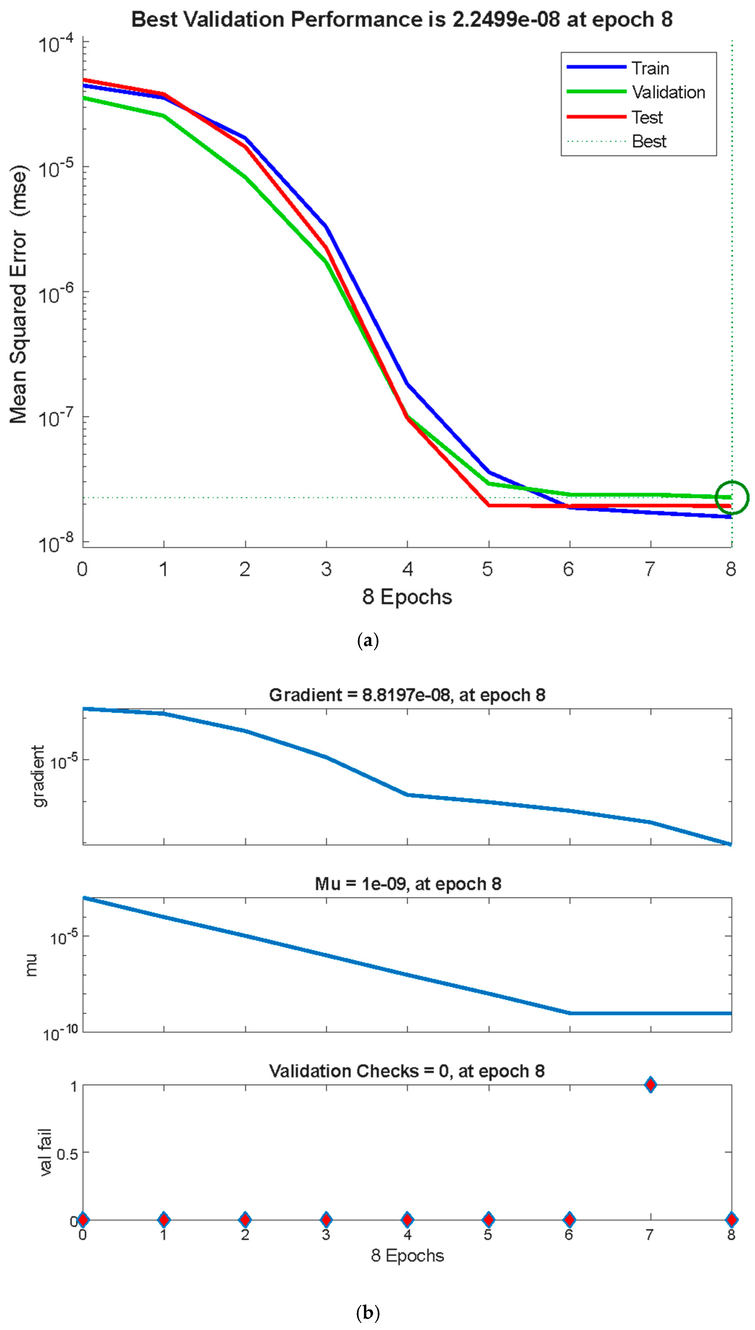
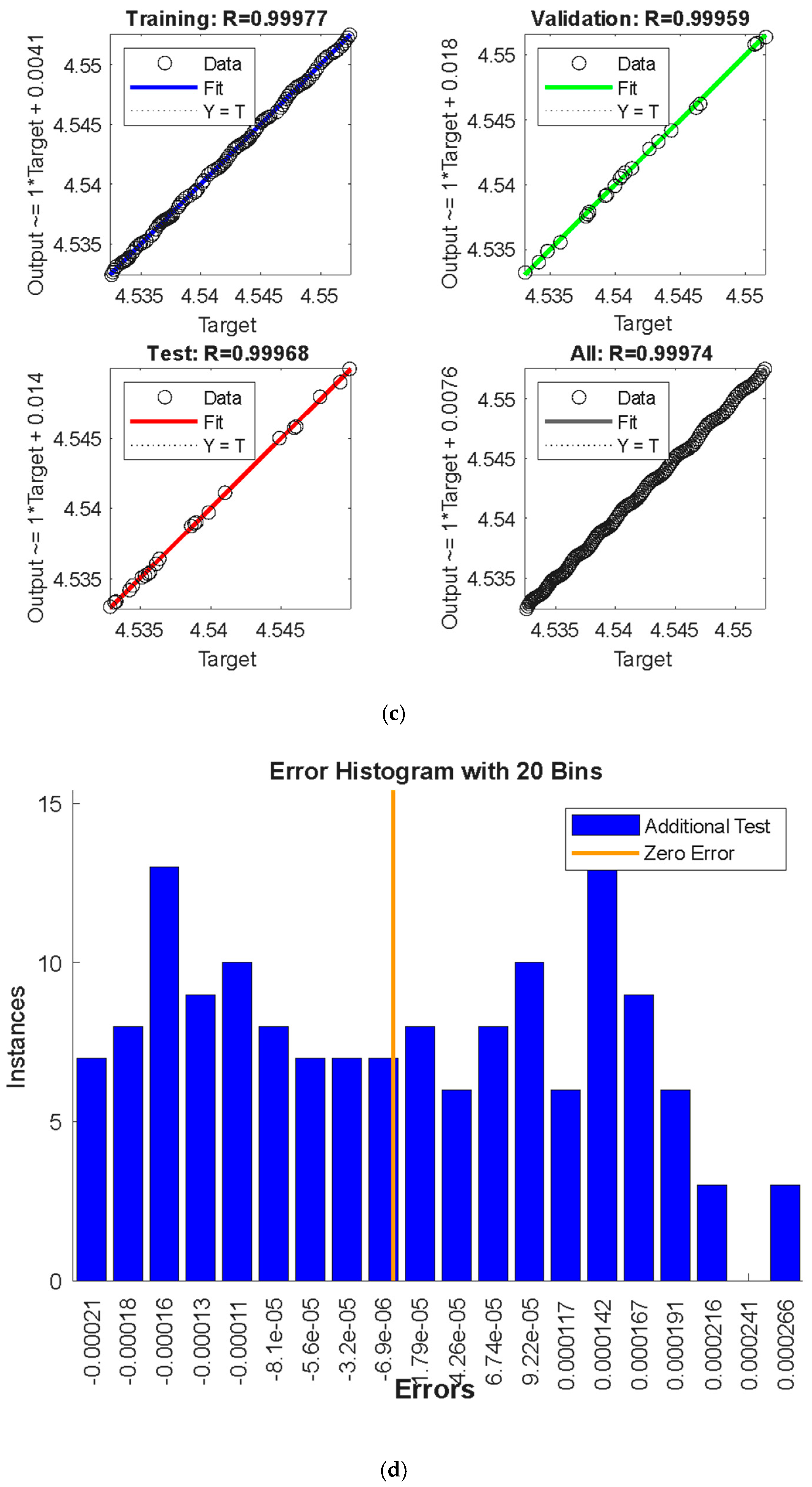
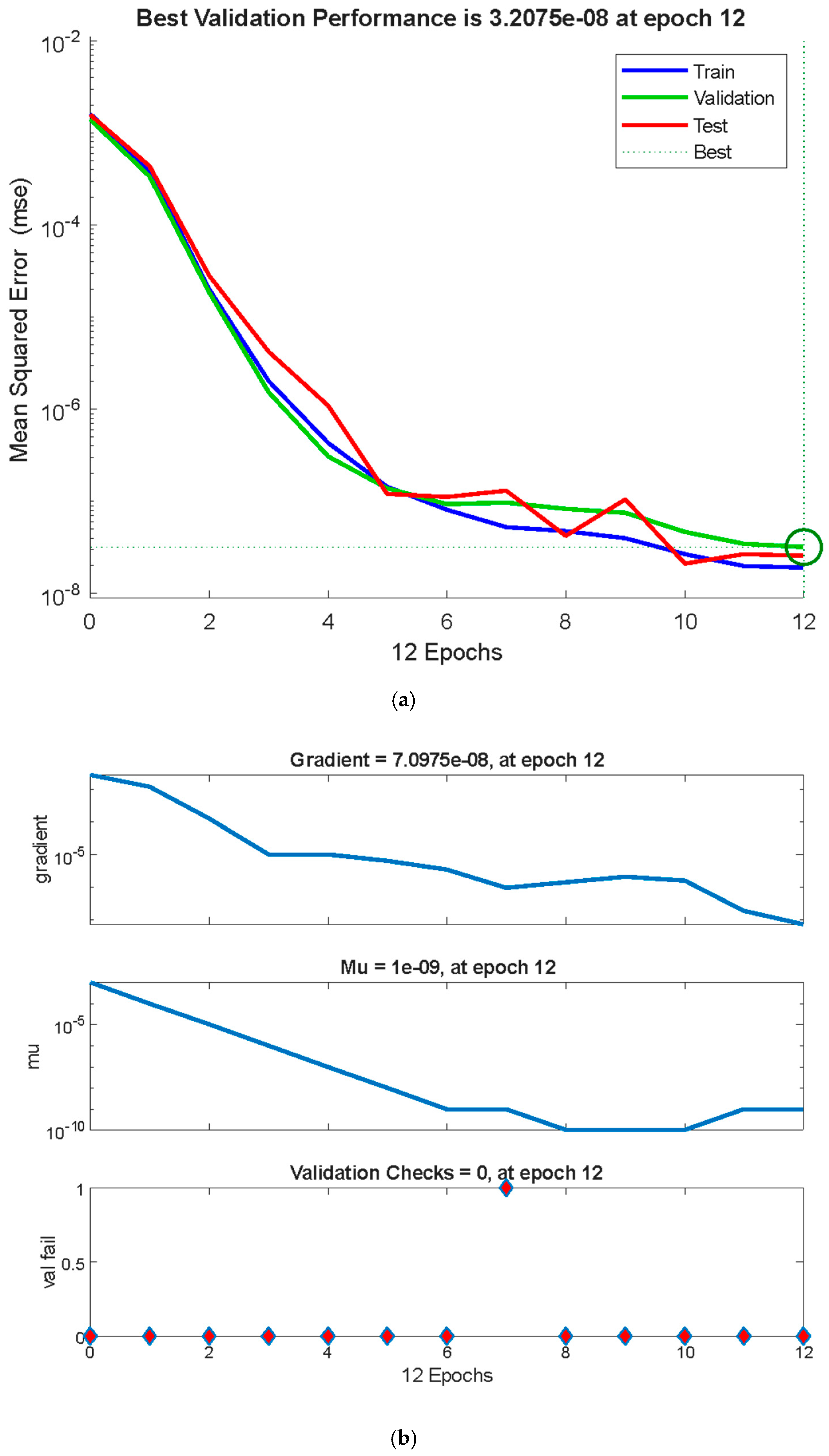
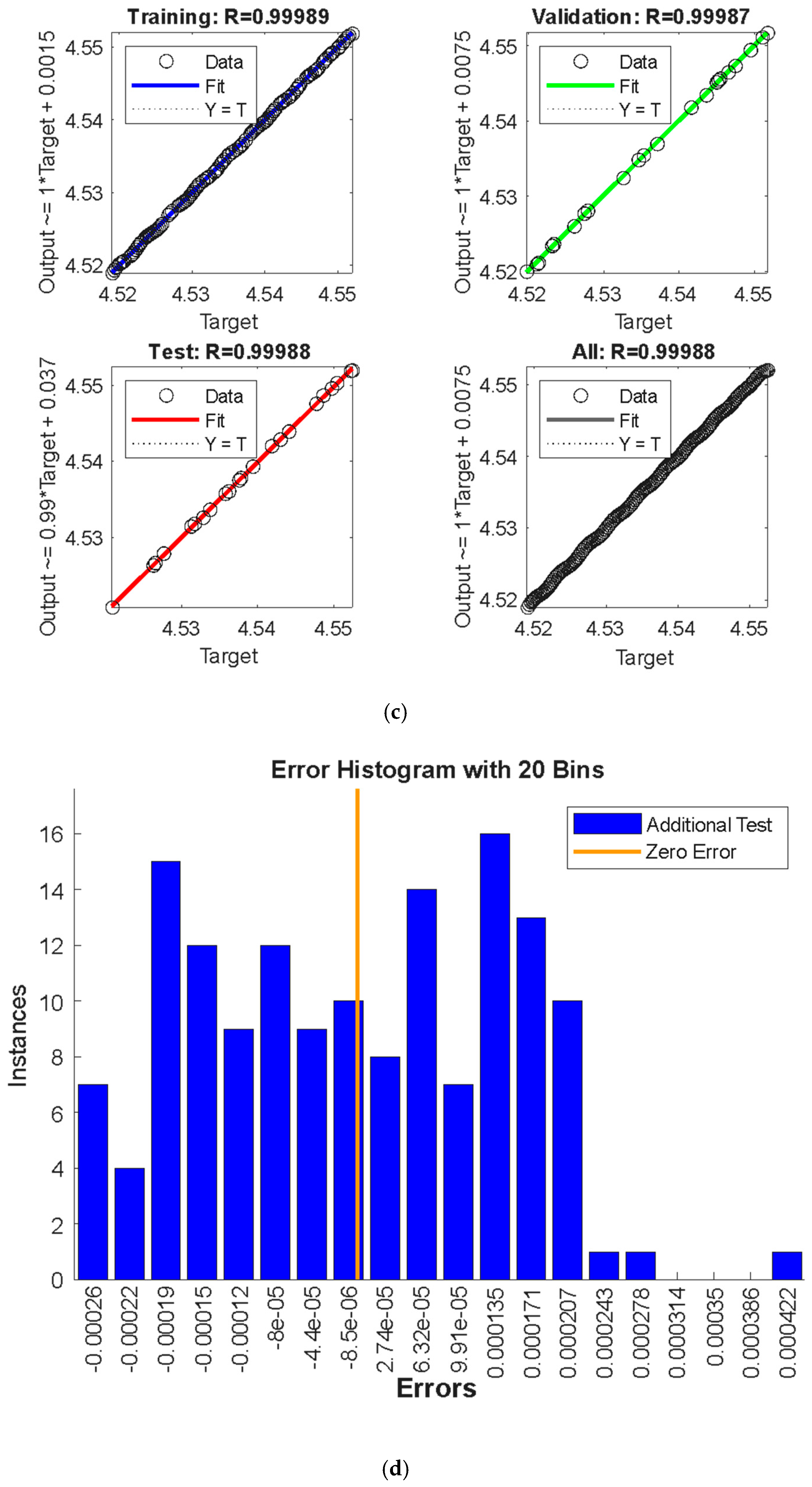
5. ANN Analysis

In this part, the ANN training model that is proposed by Levenberg–Marquardt is applied against the values of the average Nusselt coefficient for three effective parameters, namely the Reynolds number $Re$, the heat transfer coefficient $Hs$, and the heat generation coefficient $Q$. Also, the hidden layer of the ANN model is examined using the Tan-Sig function. Furthermore, the mathematical formula for the Mean Square Error (MSE), the Coefficient of Determination (R) metrics, and errors between the predicted and target values is given as follows:

$$\begin{array}{l}MSE={\displaystyle \frac{1}{N}}{\displaystyle \sum _{i=1}^N{\left(X_{\exp (i)}-X_{ANN(i)}\right)}^2}, R=\sqrt{1-{\displaystyle \frac{{\displaystyle \sum _{i=1}^N{\left(X_{\exp (i)}-X_{ANN(i)}\right)}^2}}{{\displaystyle \sum _{i=1}^N{\left(X_{\exp (i)}\right)}^2}}}},\\ Error Rate (\%)=\left[{\displaystyle \frac{X_{\exp }-X_{ANN}}{X_{\exp }}}\right]\times 100\end{array}$$

Figure 22a–d show the MSE values, performance in the form of “gradients”, the control parameter “mu”, and the “validation check” of the backpropagation algorithm, regression diagram, and the error histogram, respectively, for the average Nusselt coefficient against the variations in the Reynolds number. Noticeably, the best validation performance is $4.2724\times {10}^{-10}$ at epoch 61, with the gradient equal to $9.8988\times {10}^{-8}$, mu = $1\times {10}^{-11}$ and validation check = 0 at epoch 61, and a target value of $R=1.$ Furthermore, the differences between the predicted and target values for each dataset show that the discrepancies between the target and predicted values from the ANN model are minimal, with errors clustering near the zero-error line. This suggests that the training process was completed with few errors. In the same context, Figure 23a–d illustrate the aforementioned tools for the second parameter, $Hs$. It is revealed that the best validation performance is $2.2499\times {10}^{-9}$ at epoch 8, with the gradient equal to $8.8197\times 8$, mu = $1\times {10}^{-9}$ and validation check = 0 at epoch 8, and a target value of $R=99974.$ Also, the errors between the target and predicted values are very small and it approaches the zero-error line. Furthermore, for the third parameter, $Q$, Figure 24a–d show the ANN model training and test for the average Nu coefficient. The test revealed that the best validation performance is $3.2075\times {10}^{-8}$ at epoch 12, with the gradient equal to $7.0975\times {10}^{-8}$, mu = $1\times {10}^{-9}$ and validation check = 0 at epoch 12, and a target value of $R=0.99988$. All these observations show the best-fit model for the proposed factors and indicate successful training with minimal errors. The ANN model demonstrates exceptional performance, with rapid convergence, minimal error, and strong correlation with the target values. This level of accuracy suggests that the ANN model is highly effective for predicting the system’s outputs, including the critical parameter Q. These results validate the use of the ANN for modeling and prediction in this context, providing confidence in its application to similar problems.

6. Conclusions

Various cases based on the direction of the moving edges of a double-lid-driven enclosure were examined. The irreversibility of the system in four cases considering the two-energy equation model was investigated. Here, two mathematical formulations for the entropy generation for the solid phase and fluid phase were introduced. The worked mixture is a Cu–water nanoliquid and both the size and Brownian motion of the nanoparticles were taken into account when the values of the mixture properties were computed. The methodology of the solution was based on the finite volume technique and the heat transfer rates for both the solid and fluid phases were examined. This study led to the following major outcomes:

• In Case 1, the movement of the top wall was dominant compared to the movement of the left-side wall, and the irreversibility of the solid phase concentrated near the right-side fixed edge.
• For all cases, heat generation caused improvements in the convection situation.
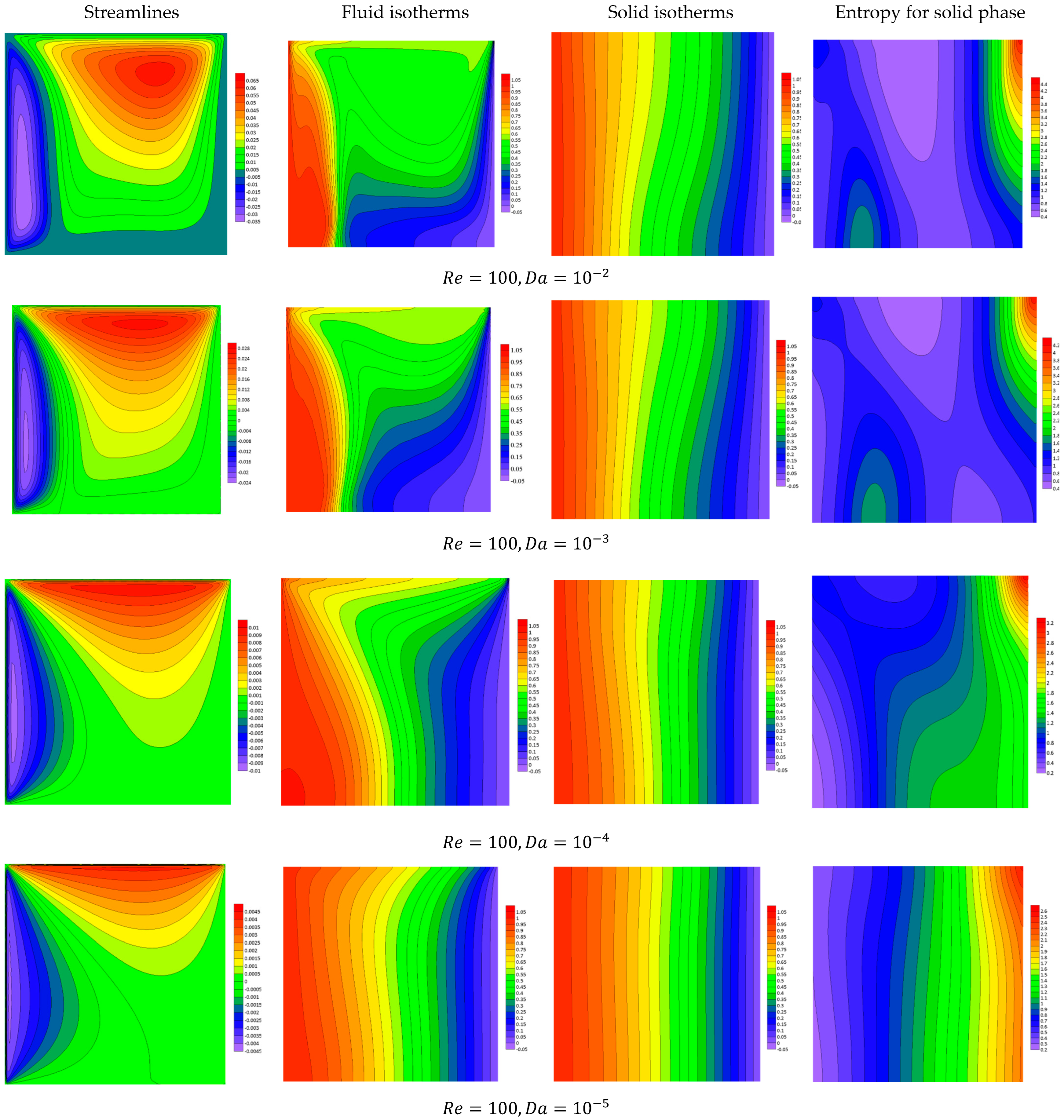
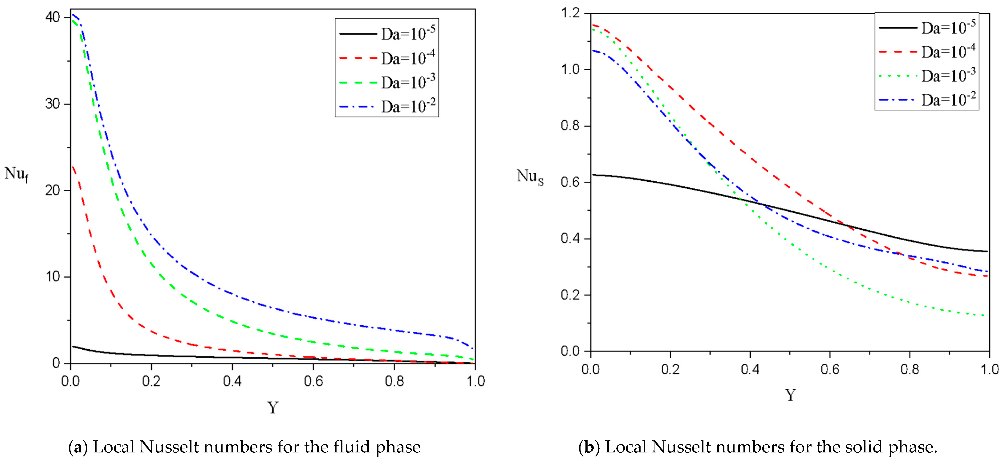
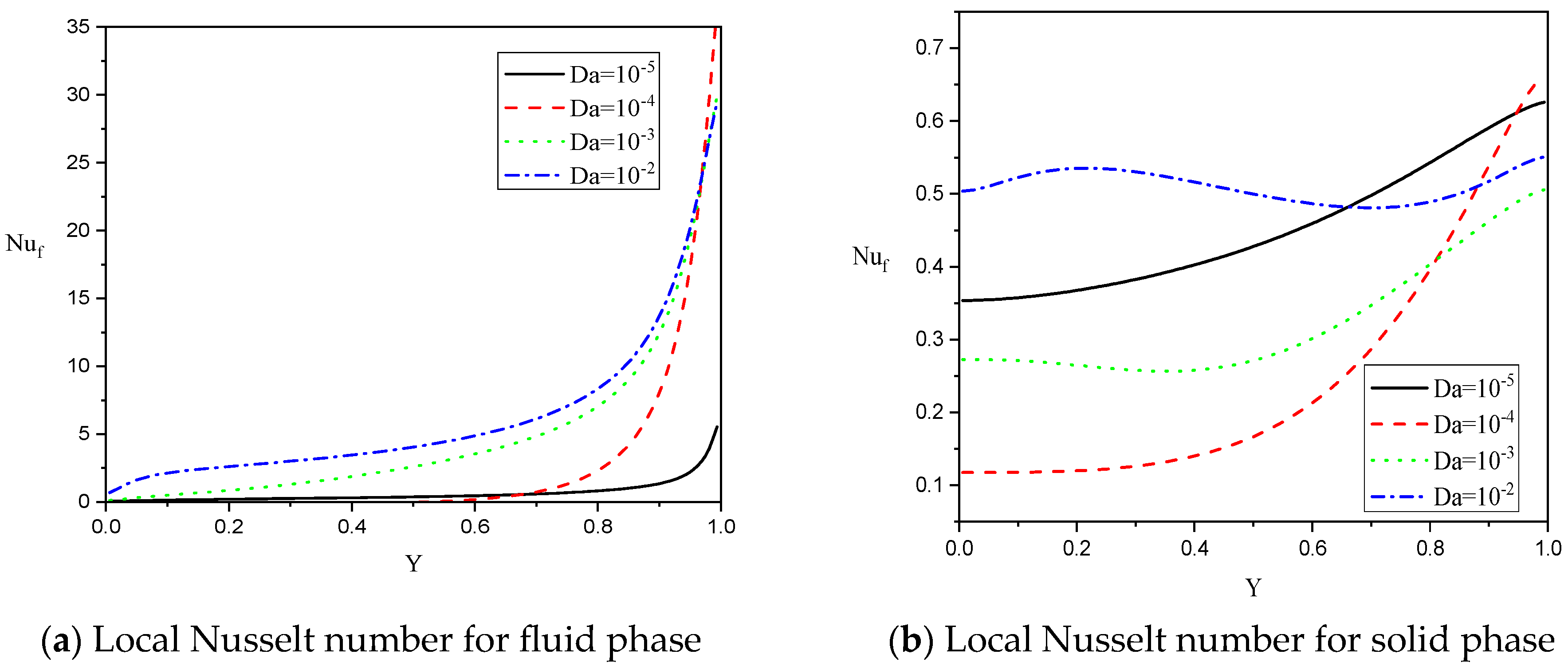
• An increase in the Darcy parameter caused diminishing flow while the heat transfer rates were improved.
• In Case 2: $U_{Y=1}=-1, V_{X=0}=1$, the minimum values of the solid phase Nusselt number occurred at the center of the wall.
• Case 3: $U_{Y=1}=1, V_{X=0}=1$ provided the highest heat transfer rates.
• In testing the flow through a porous medium, the results indicate that the LTNEM is more physically realistic compared to the LTEM.
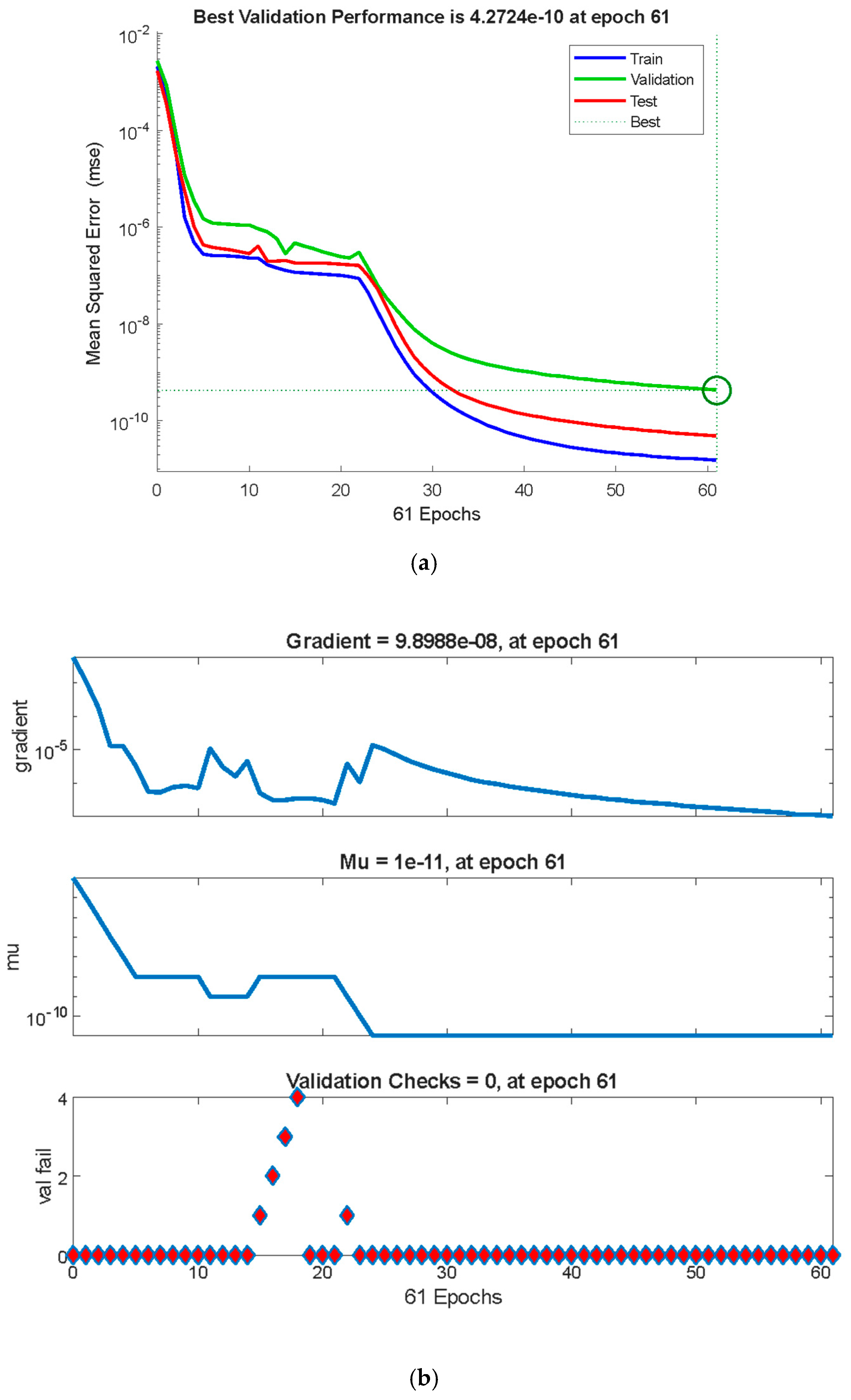
• Using the ANN model, a best-fit model for the proposed factors and successful training with minimal errors were obtained.

Finally, future research could extend the current work by investigating the effects of unsteady-state conditions on entropy generation and flow dynamics. This would provide insights into transient behavior and enhance the applicability of the findings to systems with fluctuating thermal or flow conditions.

Also, future studies could examine heterogeneous porous media with varying permeability, porosity, and thermal conductivity to better represent real-world scenarios.

Moreover, incorporating the effects of thermal radiation or magnetic fields could broaden the scope of this study, particularly for applications in solar energy systems, electromagnetic processing, or cooling of electronic components.

Future work could focus on optimizing the geometry, boundary conditions, or nanoparticle concentration to maximize thermal performance and minimize entropy generation for specific engineering applications.

Employing machine learning algorithms to predict system behavior or optimize performance parameters based on the results of this study could pave the way for data-driven design and analysis in thermal systems.

References

- Nield, D.A.; Bejan, A. Convection in Porous Media; Springer: Berlin/Heidelberg, Germany, 2006. [Google Scholar]
- Bear, J. Dynamics of Fluids in Porous Media; Dover Publications: Mineola, NY, USA, 1972. [Google Scholar]
- Vafai, K. (Ed.) Handbook of Porous Media; CRC Press: Boca Raton, FL, USA, 2005. [Google Scholar]
- Ingham, D.B.; Pop, I. (Eds.) Transport Phenomena in Porous Media; Elsevier: Amsterdam, The Netherlands, 1998. [Google Scholar]
- Kaviany, M. Principles of Heat Transfer in Porous Media; Springer: Berlin/Heidelberg, Germany, 1995. [Google Scholar]
- Choi SU, S.; Eastman, J.A. Enhancing Thermal Conductivity of Fluids with Nanoparticles. In Developments and Applications of Non-Newtonian Flows; Siginer, D.A., Wang, H.P., Eds.; ASME: New York City, NY, USA, 1995; pp. 99–105. [Google Scholar]
- Khanafer, K.; Vafai, K.; Lightstone, M. Buoyancy-driven heat transfer enhancement in a two-dimensional enclosure utilizing nanofluids. Int. J. Heat Mass Transf. 2003, 46, 3639–3653. [Google Scholar] [CrossRef]
- Brinkman, H.C. The viscosity of concentrated suspensions and solutions. J. Chem. Phys. 1952, 20, 571–581. [Google Scholar] [CrossRef]
- Buongiorno, J. Convective transport in nanofluids. J. Heat Transf. 2006, 128, 240–250. [Google Scholar] [CrossRef]
- Xuan, Y.; Li, Q. Heat transfer enhancement of nanofluids. Int. J. Heat Fluid Flow 2000, 21, 58–64. [Google Scholar] [CrossRef]
- Ho, C.J.; Chen, M.W.; Li, Z.W. Numerical simulation of natural convection of nanofluid in a square enclosure: Effect due to uncertainties of viscosity and thermal conductivity. Int. J. Heat Mass Transf. 2008, 51, 4506–4516. [Google Scholar] [CrossRef]
- Talebi, F.; Mahmoudi, A.H.; Shahi, M. Numerical study of mixed convection flows in a square lid-driven cavity utilizing nanofluid. Int. Commun. Heat Mass Transf. 2010, 37, 79–90. [Google Scholar] [CrossRef]
- Torabi, M.; Zhang, K.; Yang, G.; Wang, J.; Wu, P. Heat transfer and entropy generation analyses in a channel partially filled with porous media using local thermal non-equilibrium model. Energy 2015, 82, 922–938. [Google Scholar] [CrossRef]
- Kim, S.J.; Hyun, J.M. A porous medium approach for the thermal analysis of heat transfer devices. In Transport Phenomena in Porous Media III; Ingham, D.B., Pop, I., Eds.; Pergamon: Oxford, UK, 2005; pp. 120–146. ISBN 9780080444901. [Google Scholar] [CrossRef]
- Ahmed, S.E.; Rashed, Z.Z.; Al-Hanaya, A. Three dimensional melting case of phase change material composited with heat generating and local thermal non-equilibrium copper foam under the magnetic impacts. Appl. Therm. Eng. 2023, 219, 119662. [Google Scholar] [CrossRef]
- Ahmed, S.E.; Raizha, Z.A. Role of sinusoidal/linearly inner heating on the irreversibility of mixed convection in split lid-driven chamfered enclosures filled with thermal non-equilibrium permeable medium. Int. J. Heat Fluid Flow 2025, 112, 109715. [Google Scholar] [CrossRef]
- Patankar, S.V. Numerical Heat Transfer and Fluid Flow; Taylor & Francis: Abingdon, UK, 1980. [Google Scholar]
- Whitaker, S. The Method of Volume Averaging; Springer Science & Business Media: Berlin, Germany, 1999. [Google Scholar]
- Parhizi, M.; Torabi, M.; Jain, A. Local thermal non-equilibrium (LTNE) model for developed flow in porous media with spatially-varying Biot number. Int. J. Heat Mass Transf. 2021, 164, 120538. [Google Scholar] [CrossRef]
- Gandomkar, A.; Gray, K.E. Local thermal non-equilibrium in porous media with heat conduction. Int. J. Heat Mass Transf. 2018, 124, 1212–1216. [Google Scholar] [CrossRef]
- Badruddin, I.A. Numerical Analysis of Thermal Non-Equilibrium in Porous Medium Subjected to Internal Heating. Mathematics 2019, 7, 1085. [Google Scholar] [CrossRef]
- Ahmed, S.E.; Raizha, Z.A.S.; Alsubaie, F. Artificial neural network and CBS-FEM techniques for mixed convection in lid-driven tank heated by triangular fins and filled with permeable medium: Two-energy equations model. J. Taiwan Inst. Chem. Eng. 2025, 167, 105850. [Google Scholar] [CrossRef]
- Bejan, A. Entropy Generation Minimization: The Method of Thermodynamic Optimization of Finite-Size Systems and Finite-Time Processes; CRC Press: Boca Raton, FL, USA, 1996. [Google Scholar]
- Kuznetsov, A.V.; Nield, D.A. The effects of local thermal non-equilibrium on convection in a porous medium. Int. J. Heat Mass Transf. 2010, 53, 315–321. [Google Scholar]
- Mahapatra, T.R.; Panda, S.; Das, P.K. Numerical investigation on mixed convection and entropy generation in a porous cavity. J. Therm. Sci. Eng. Appl. 2016, 8, 041008. [Google Scholar]
- Barletta, A.; Rees DA, S.; Storesletten, L. Mixed convection in porous media: Mathematical models and scale analysis. Transp. Porous Media 2018, 123, 317–343. [Google Scholar]
- Rashidi, M.M.; Chamkha, A.J.; Yang, Z. Entropy generation in porous cavities with thermal and flow boundary conditions. Numer. Heat Transf. Part A Appl. 2019, 76, 567–583. [Google Scholar]
- Tiwari, R.K.; Das, M.K. Heat transfer augmentation in a two-sided lid-driven differentially heated square cavity utilizing nanofluids. Int. J. Heat Mass Transf. 2007, 50, 2002–2201. [Google Scholar] [CrossRef]
- Tayebi, T. Analysis of the local non-equilibria on the heat transfer and entropy generation during thermal natural convection in a non-Darcy porous medium. Int. Commun. Heat Mass Transf. 2022, 135, 106133. [Google Scholar] [CrossRef]
- Iwatsu, R.; Hyun, J.M.; Kuwahara, K. Mixed convection in a driven cavity with a stable vertical temperature gradient. Int. J. Heat Mass Transf. 1993, 36, 1601–1608. [Google Scholar] [CrossRef]
- Khanafer, K.M.; Chamkha, A.J. Mixed convection flow in a lid-driven enclosure filled with a fluid-saturated porous medium. Int. J. Heat Mass Transf. 1999, 31, 1354–1370. [Google Scholar] [CrossRef]