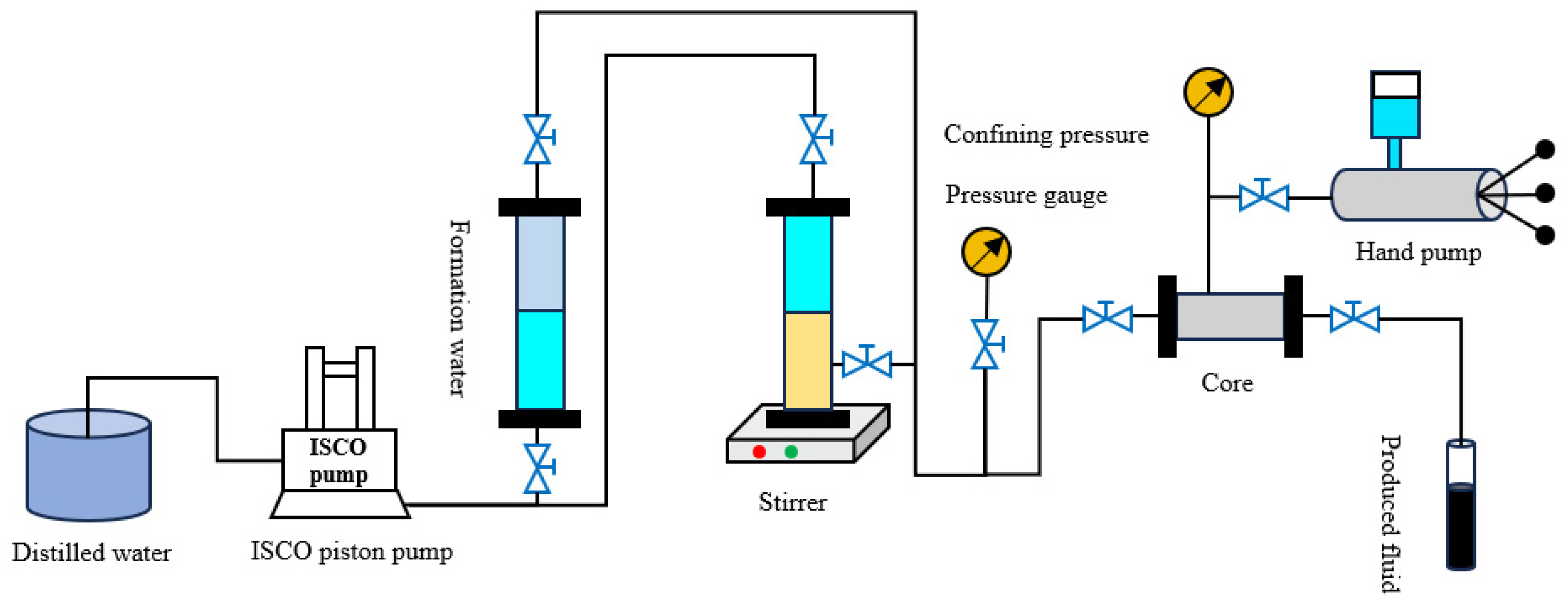
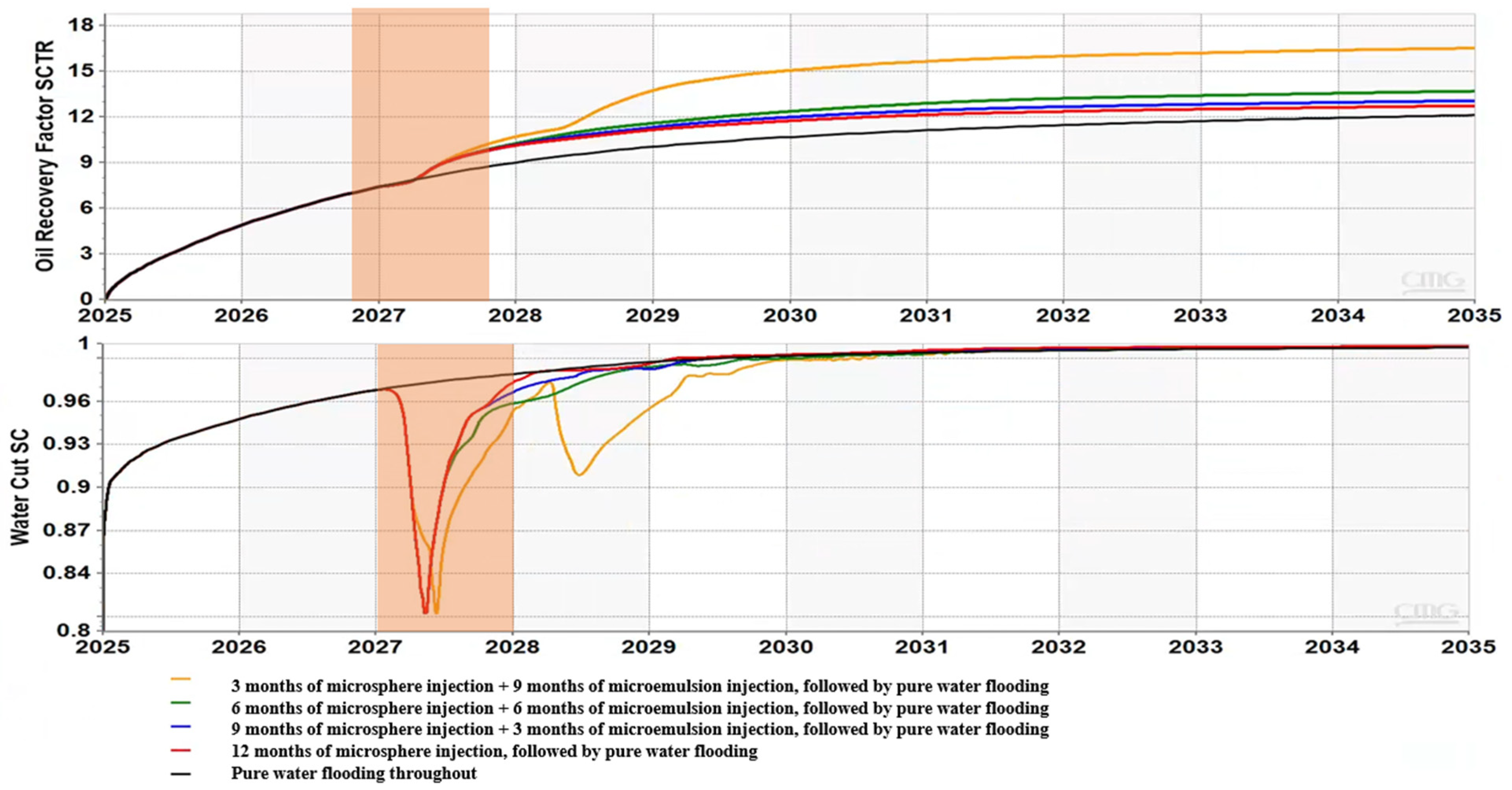
Figure 1.
Core-flood experimental flow chart.
Figure 1.
Core-flood experimental flow chart.
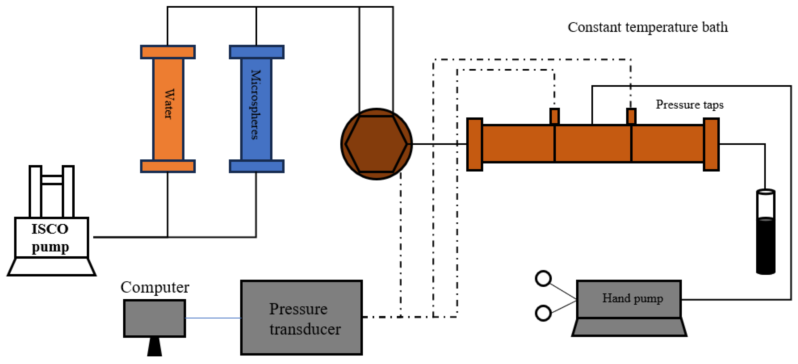
Figure 2.
Core-flooding apparatus.
Figure 2.
Core-flooding apparatus.
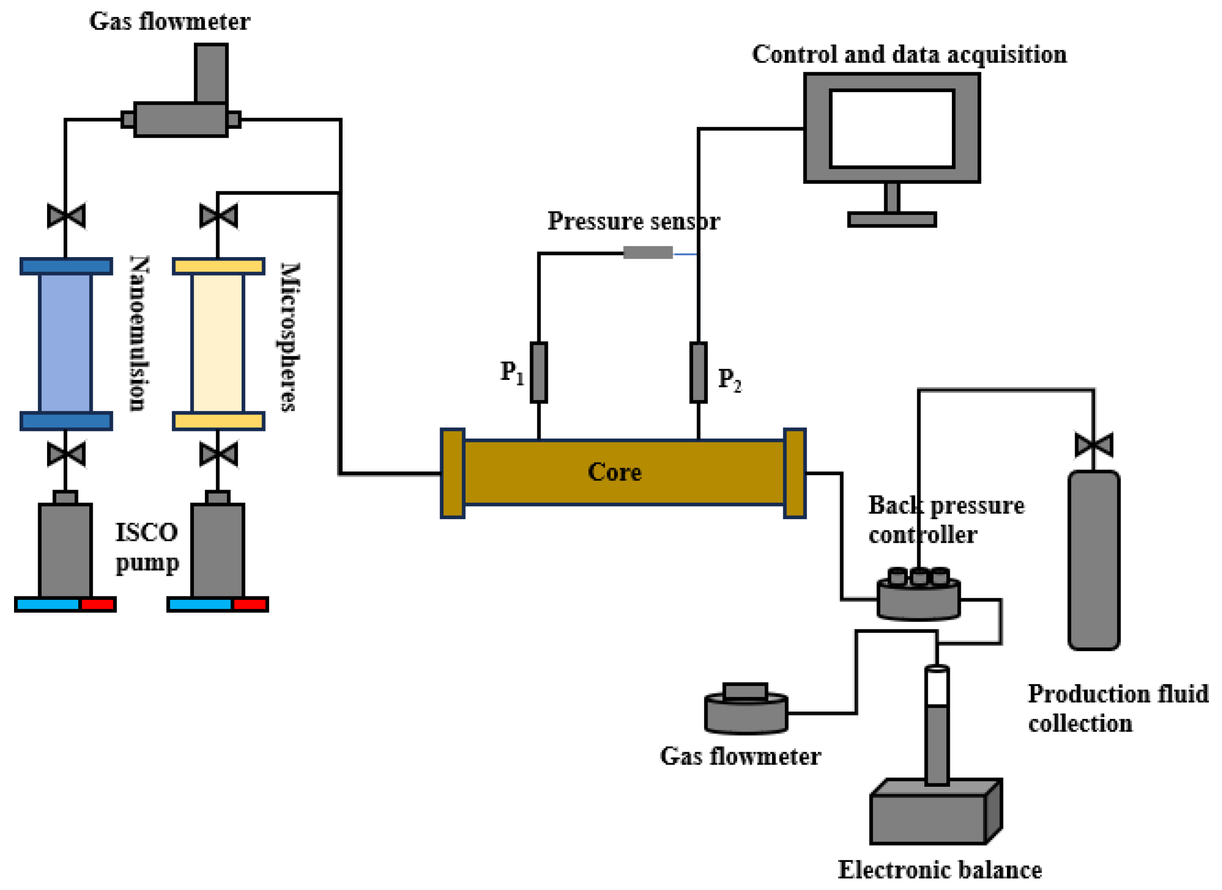
Figure 3.
Single-core flooding set-up.
Figure 3.
Single-core flooding set-up.
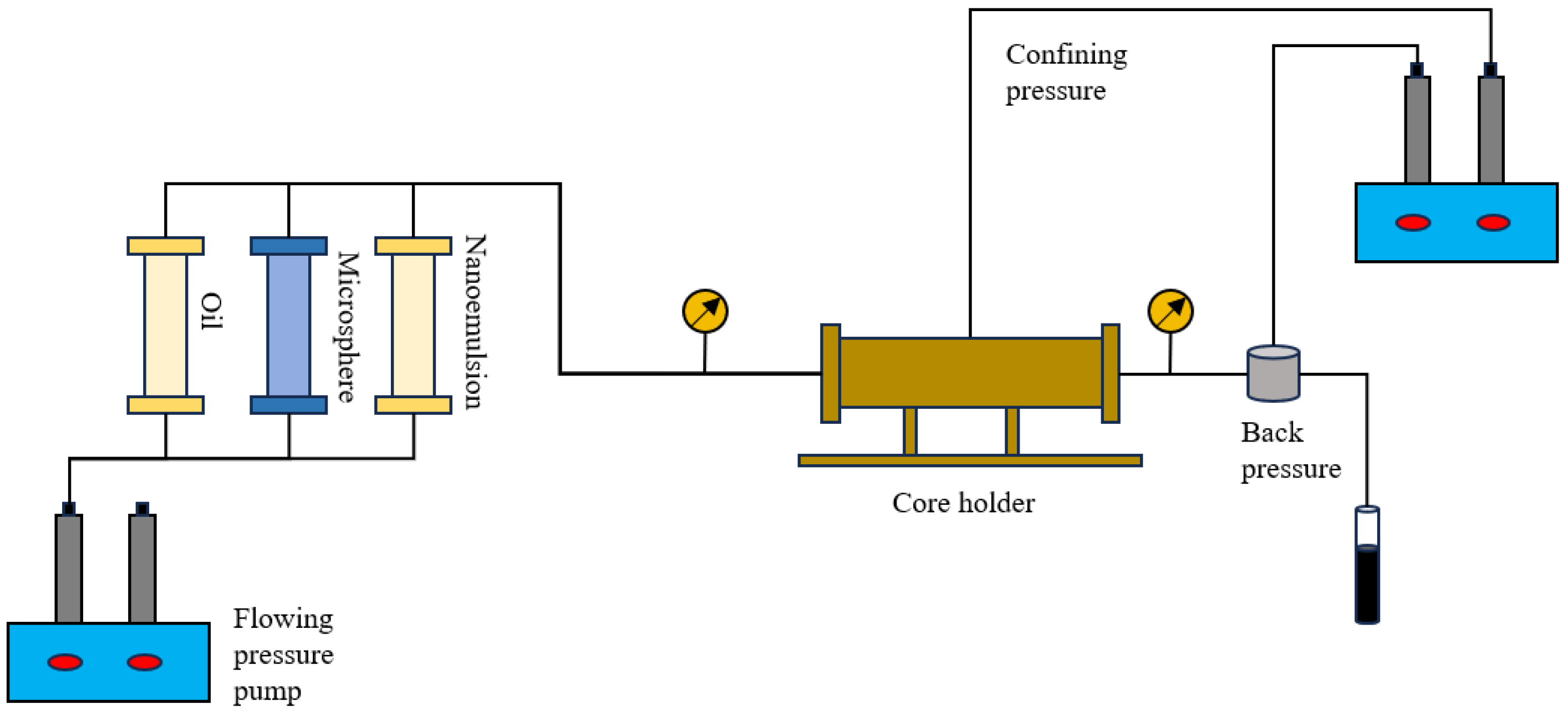
Figure 4.
Dual-core flooding apparatus.
Figure 4.
Dual-core flooding apparatus.
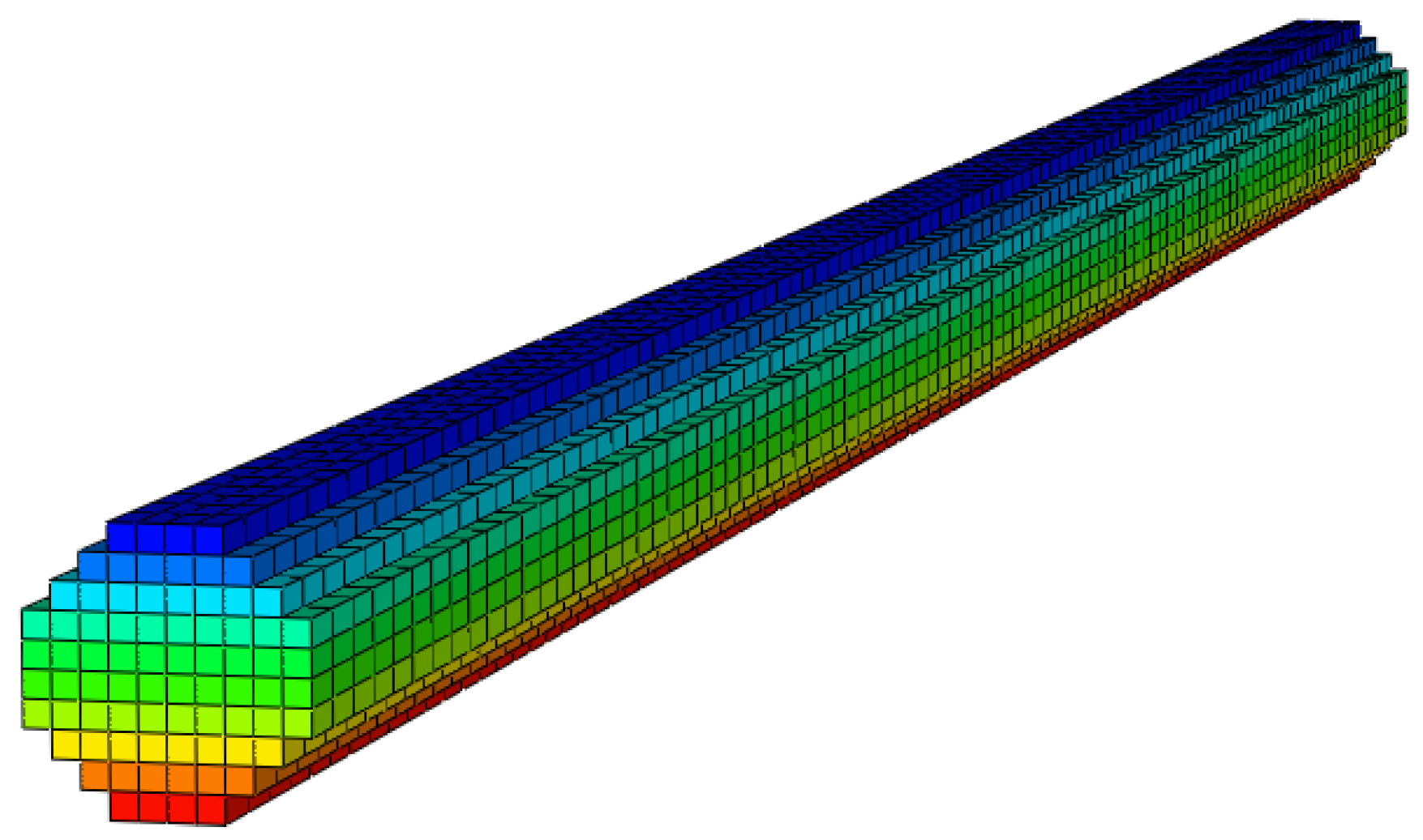
Figure 5.
Core-scale numerical model.
Figure 5.
Core-scale numerical model.
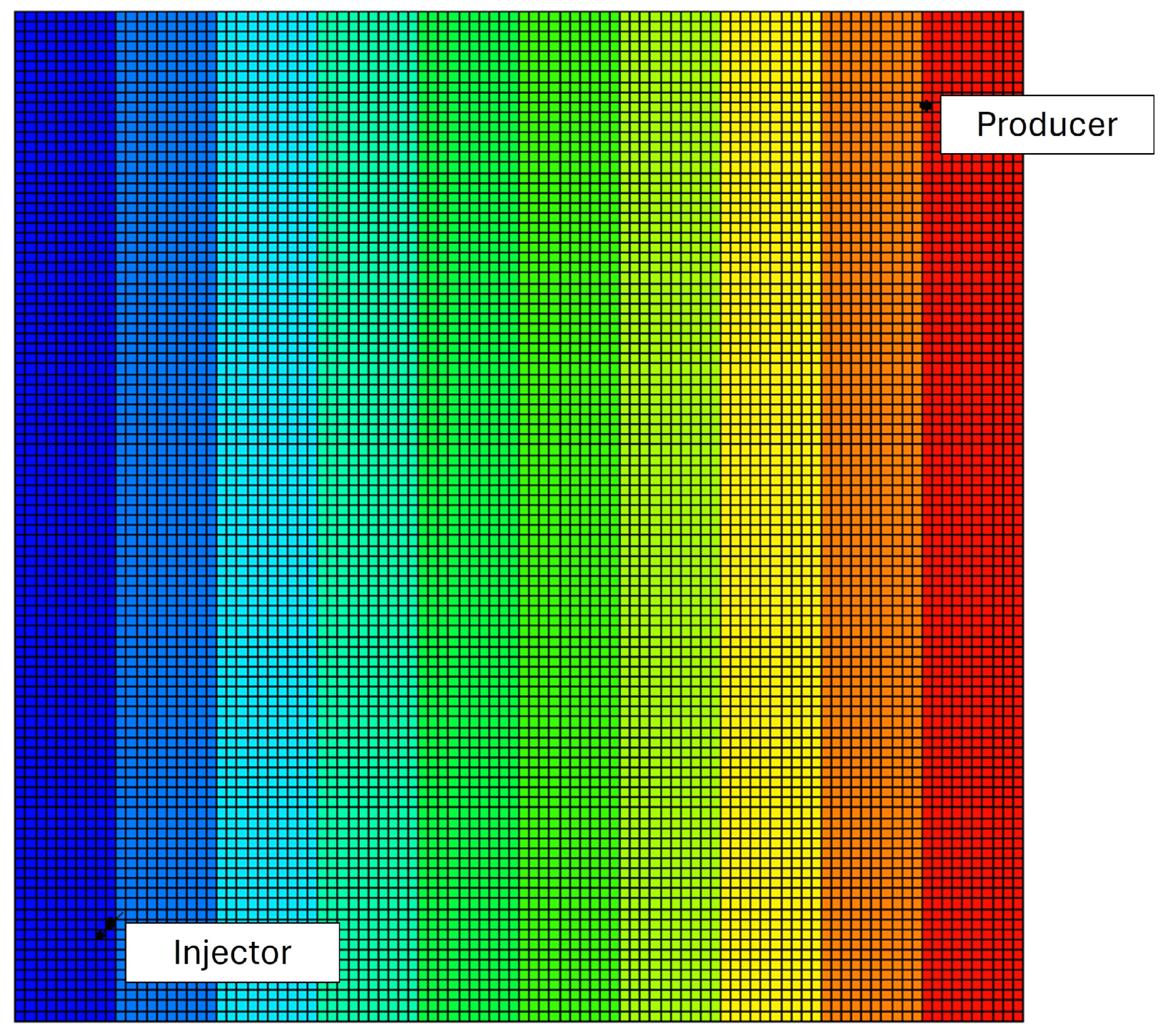
Figure 6.
Well-pattern-scale homogeneous reservoir model.
Figure 6.
Well-pattern-scale homogeneous reservoir model.
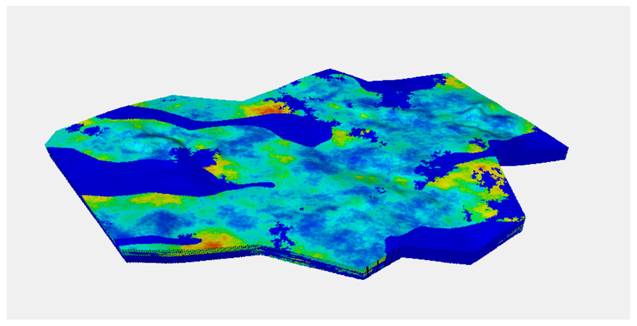
Figure 7.
Full-field reservoir numerical model.
Figure 7.
Full-field reservoir numerical model.
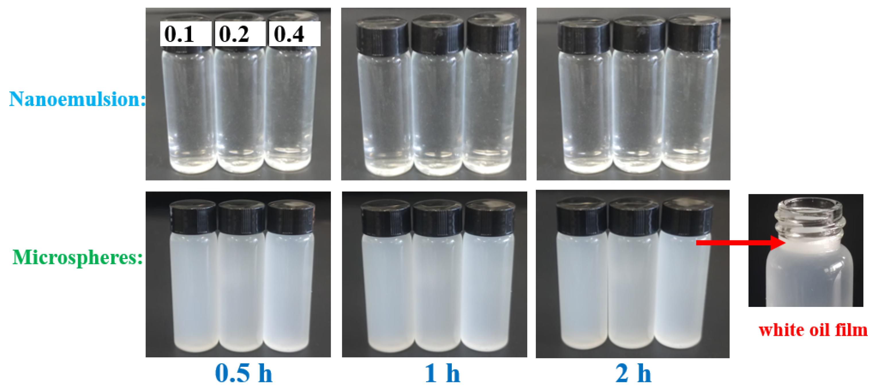
Figure 8.
Macroscopic observation of dispersion stability.
Figure 8.
Macroscopic observation of dispersion stability.
Figure 9.
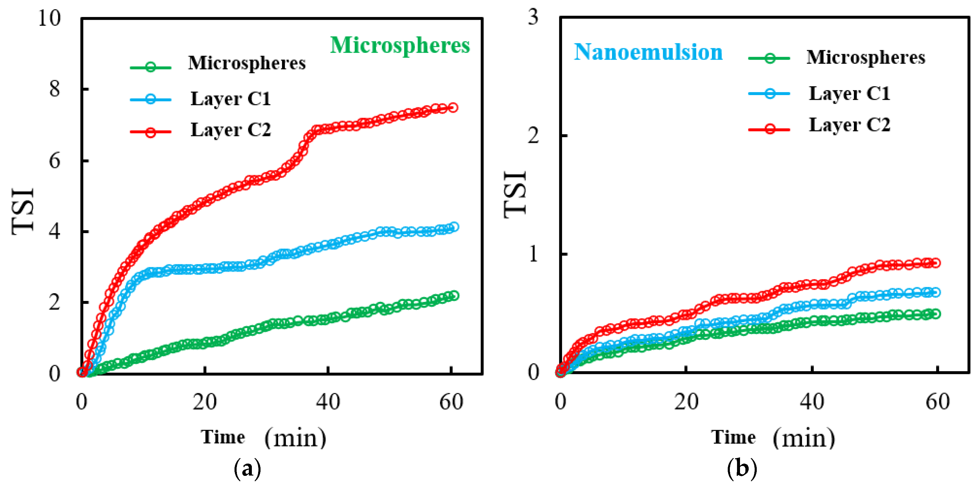
Stability index under different reservoir conditions. (a) Microspheres 2.0; (b) Nanoemulsion.
Figure 9.
Stability index under different reservoir conditions. (a) Microspheres 2.0; (b) Nanoemulsion.
Figure 10.
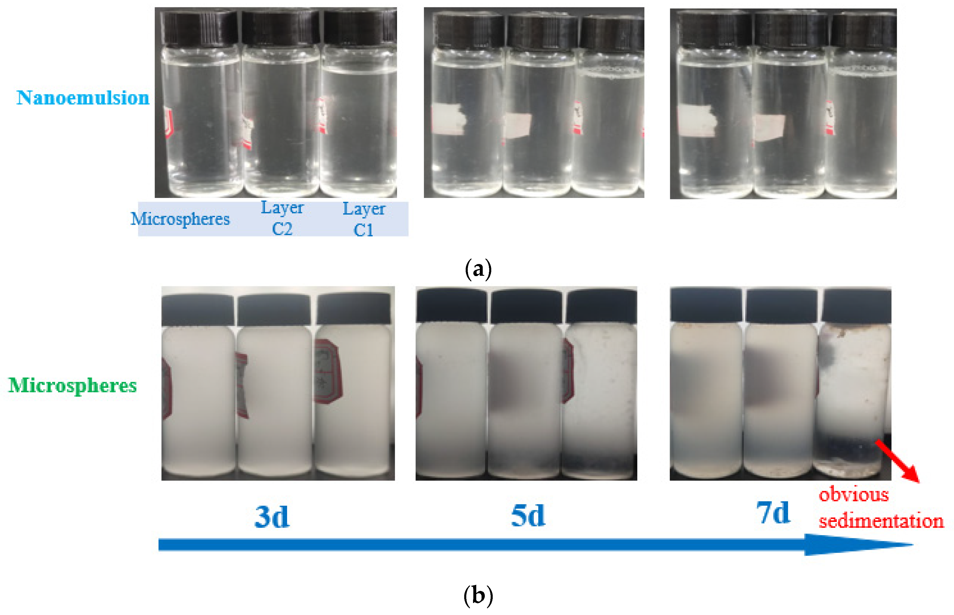
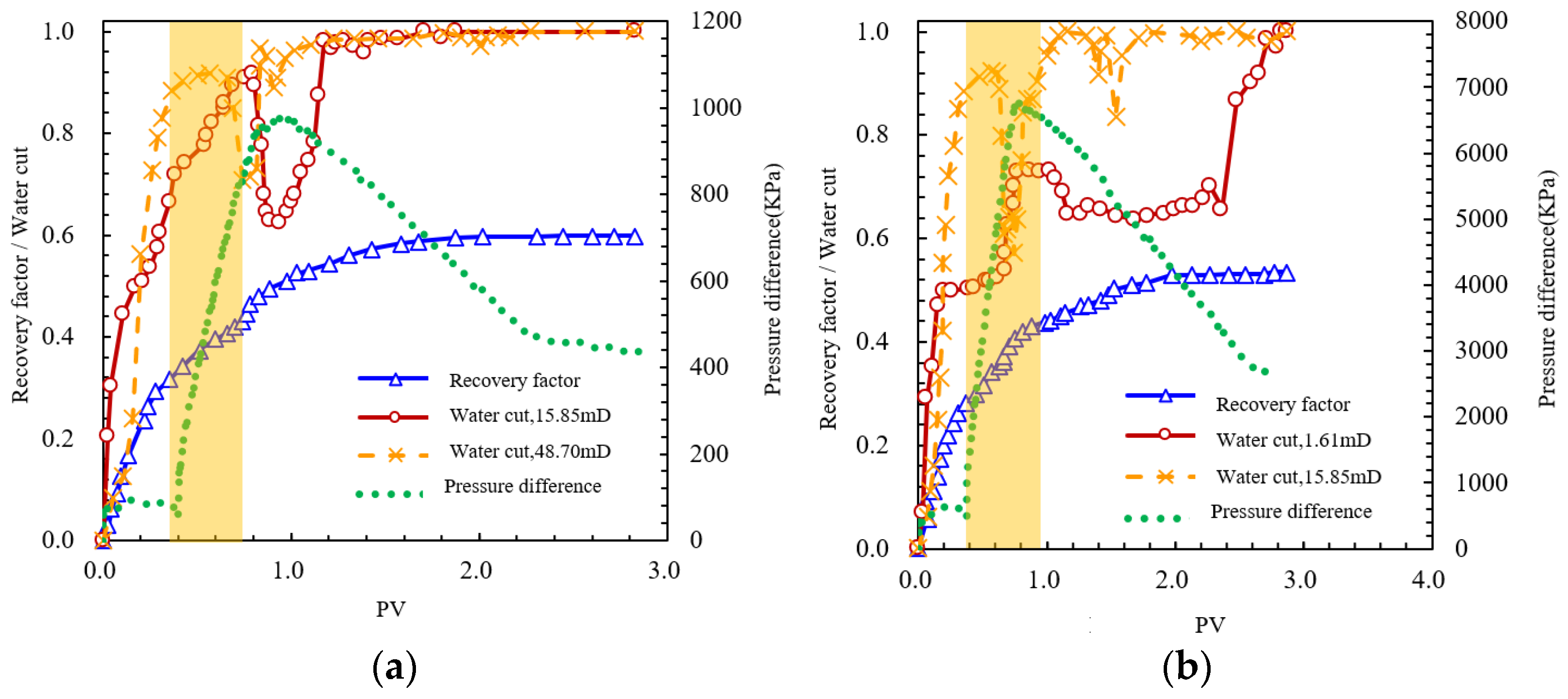
Aging morphology of microspheres and nanoemulsion. (a) Nanoemulsion; (b) Microspheres 2.0.
Figure 10.
Aging morphology of microspheres and nanoemulsion. (a) Nanoemulsion; (b) Microspheres 2.0.
Figure 11.
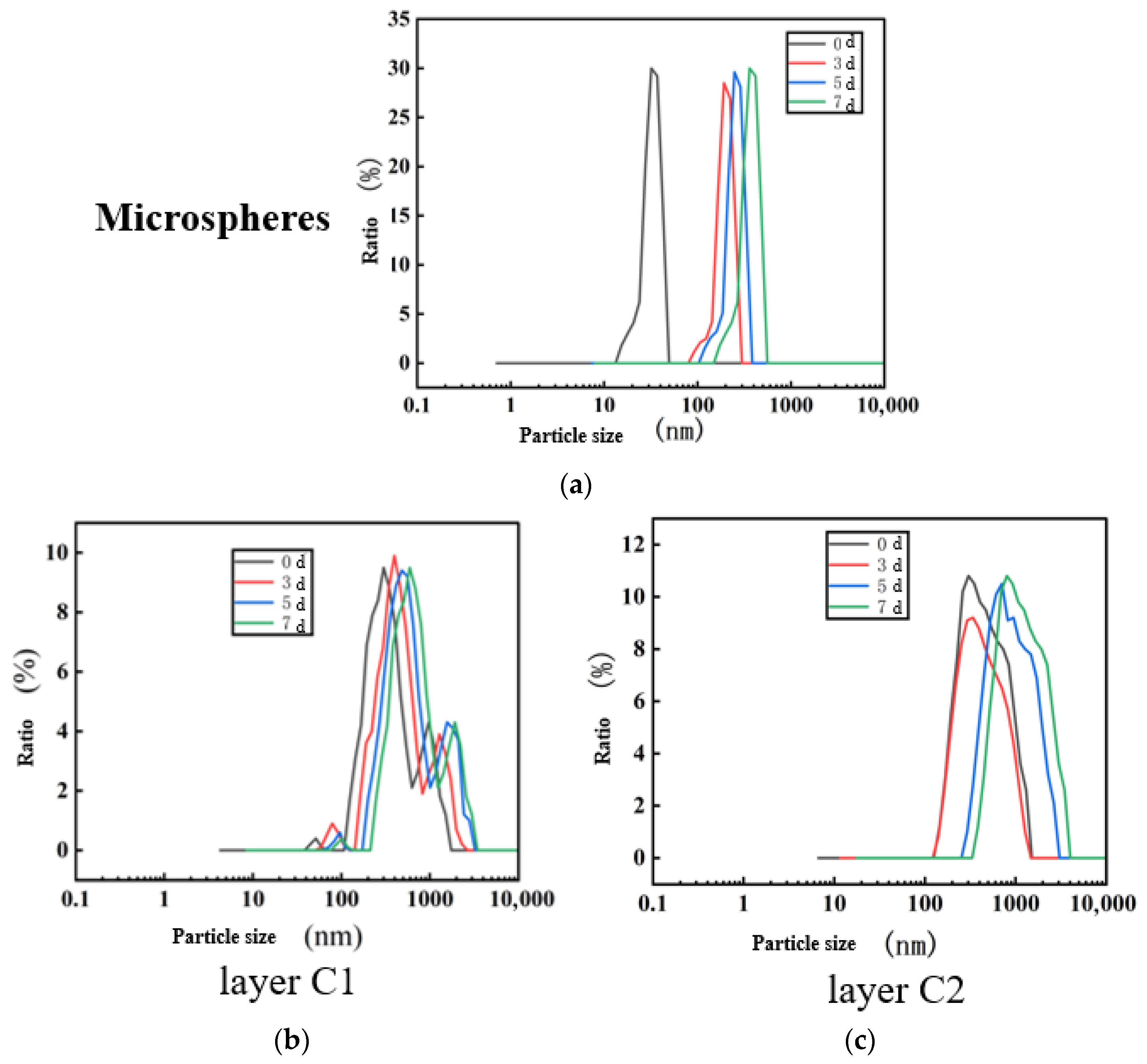
Particle-size distribution of nanoemulsion in different systems. (a) Microspheres; (b) Layer C1; (c) Layer C2.
Figure 11.
Particle-size distribution of nanoemulsion in different systems. (a) Microspheres; (b) Layer C1; (c) Layer C2.
Figure 12.
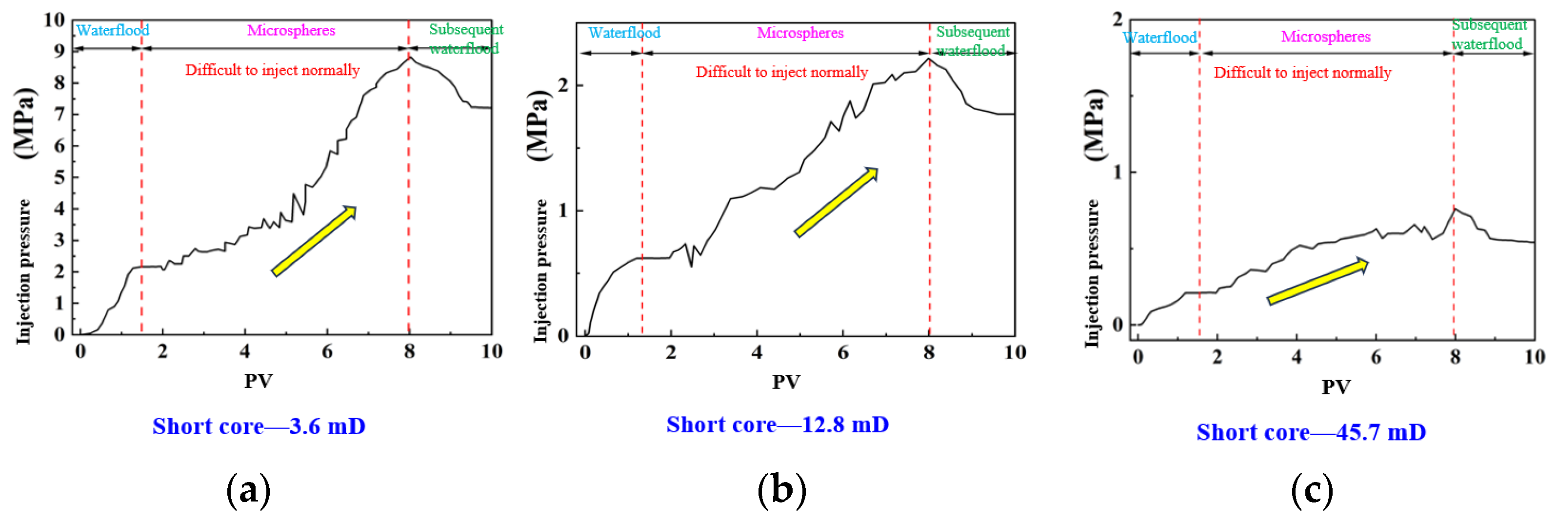
Injection pressure versus injected volume for systems of different permeability. (a) 3.6 mD; (b) 12.8 mD; (c) 45.7 mD.
Figure 12.
Injection pressure versus injected volume for systems of different permeability. (a) 3.6 mD; (b) 12.8 mD; (c) 45.7 mD.
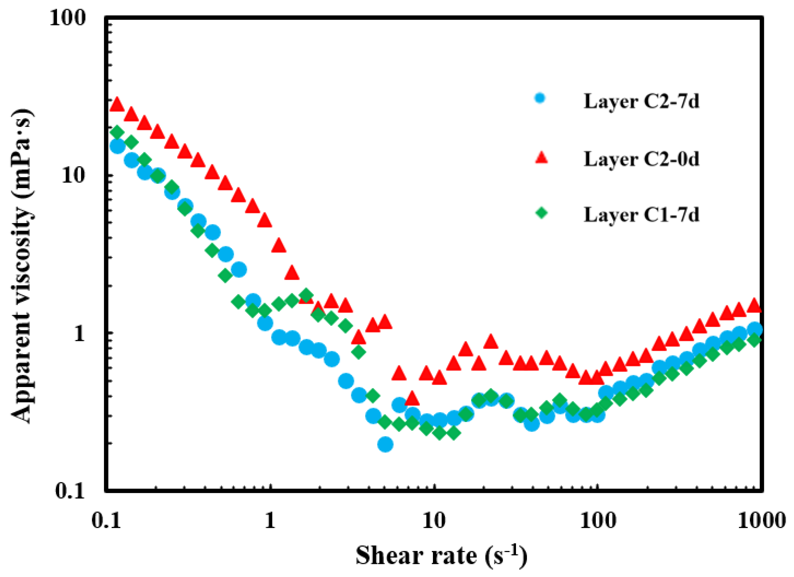
Figure 13.
Apparent viscosity versus shear rate.
Figure 13.
Apparent viscosity versus shear rate.
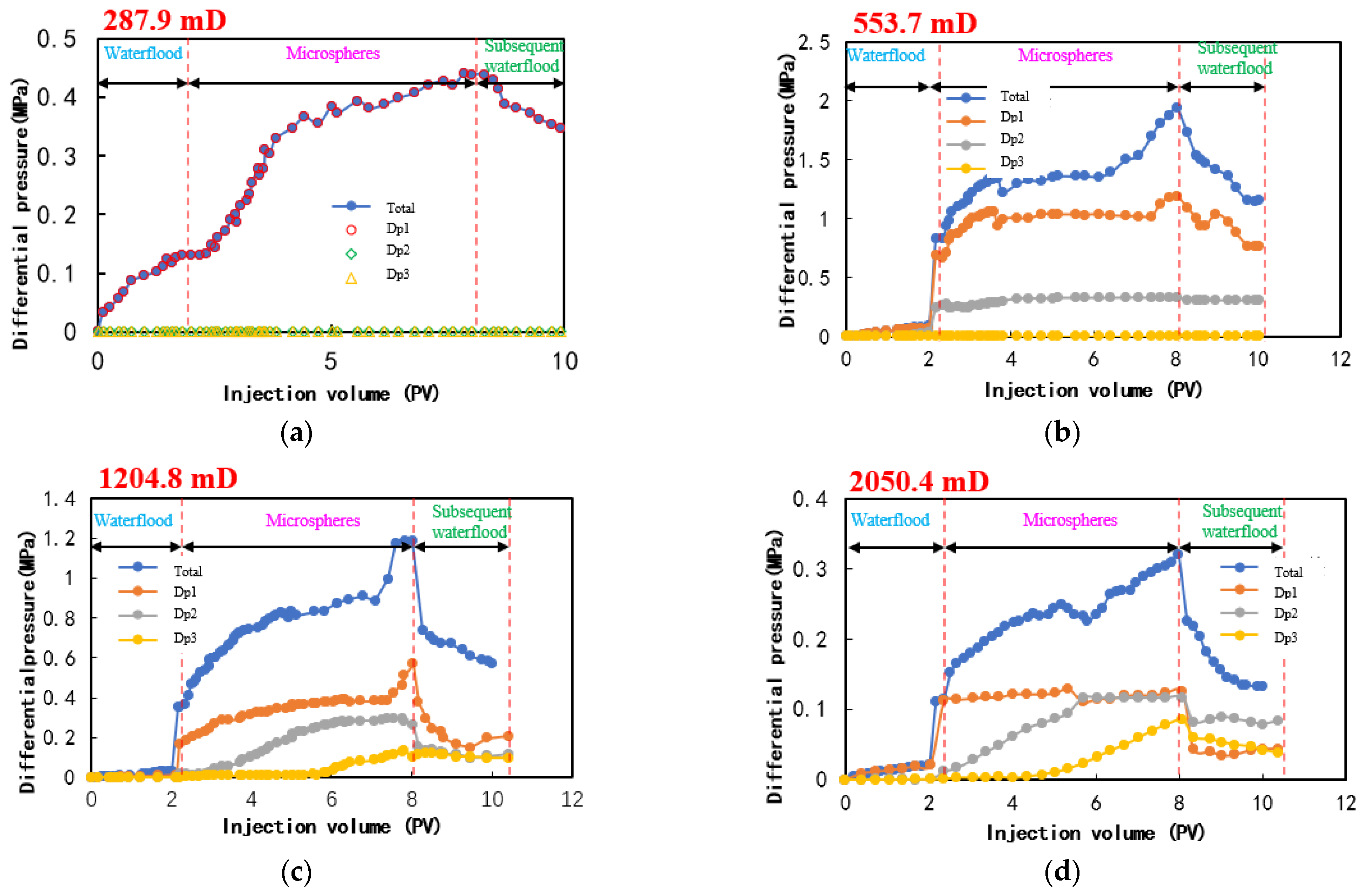
Figure 14.
Four plugging-type profiles. (a) 287.9 mD; (b) 553.7 mD; (c) 1204.8 mD (d) 2050.4 mD.
Figure 14.
Four plugging-type profiles. (a) 287.9 mD; (b) 553.7 mD; (c) 1204.8 mD (d) 2050.4 mD.
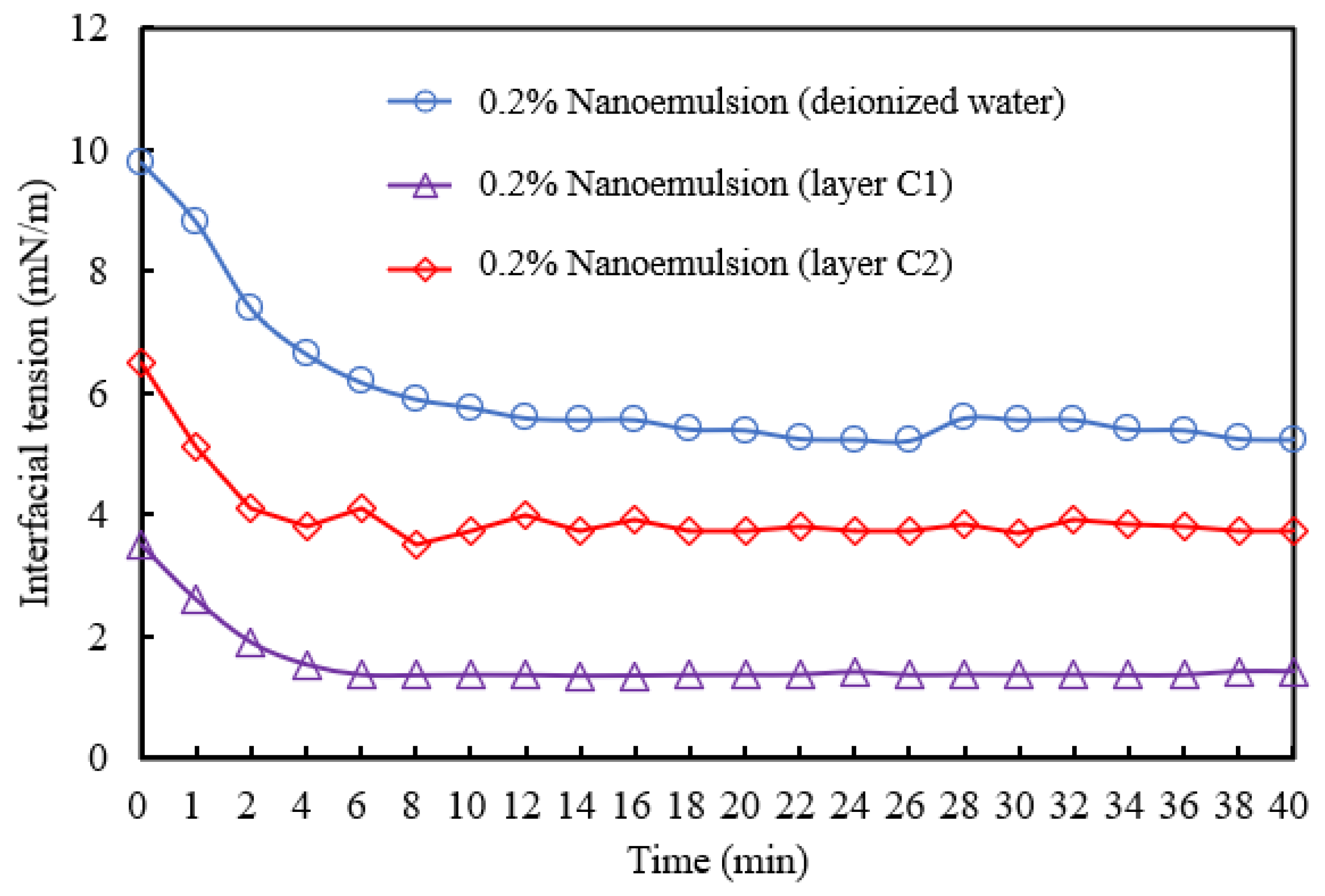
Figure 15.
Dynamic oil–water interfacial tension profiles.
Figure 15.
Dynamic oil–water interfacial tension profiles.
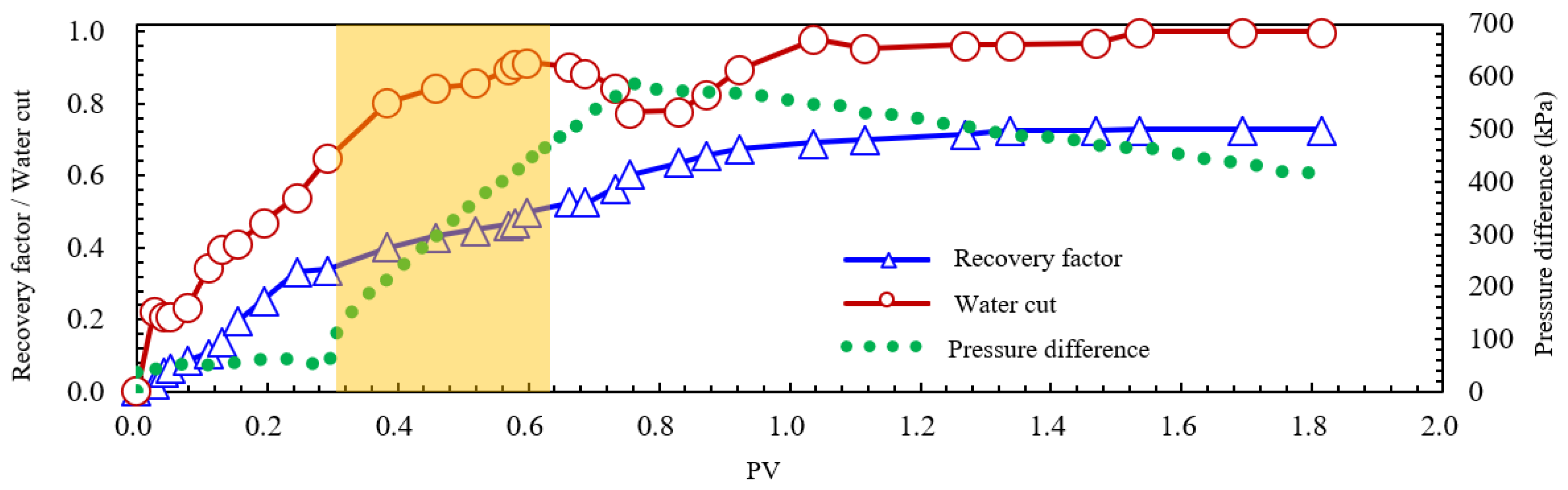
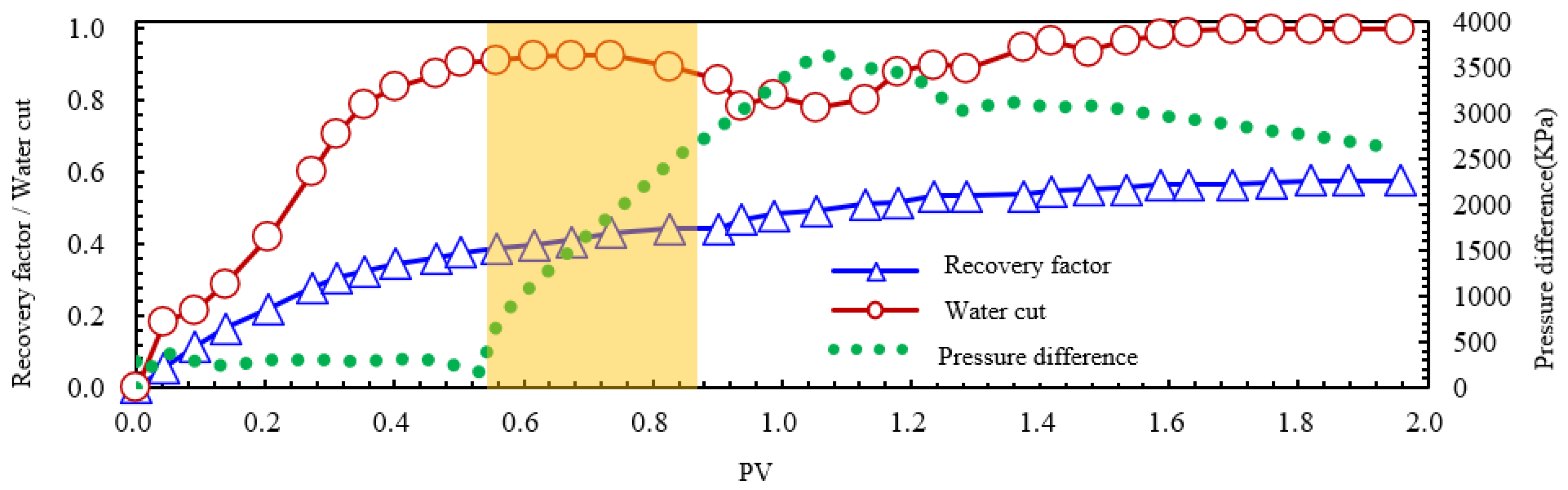
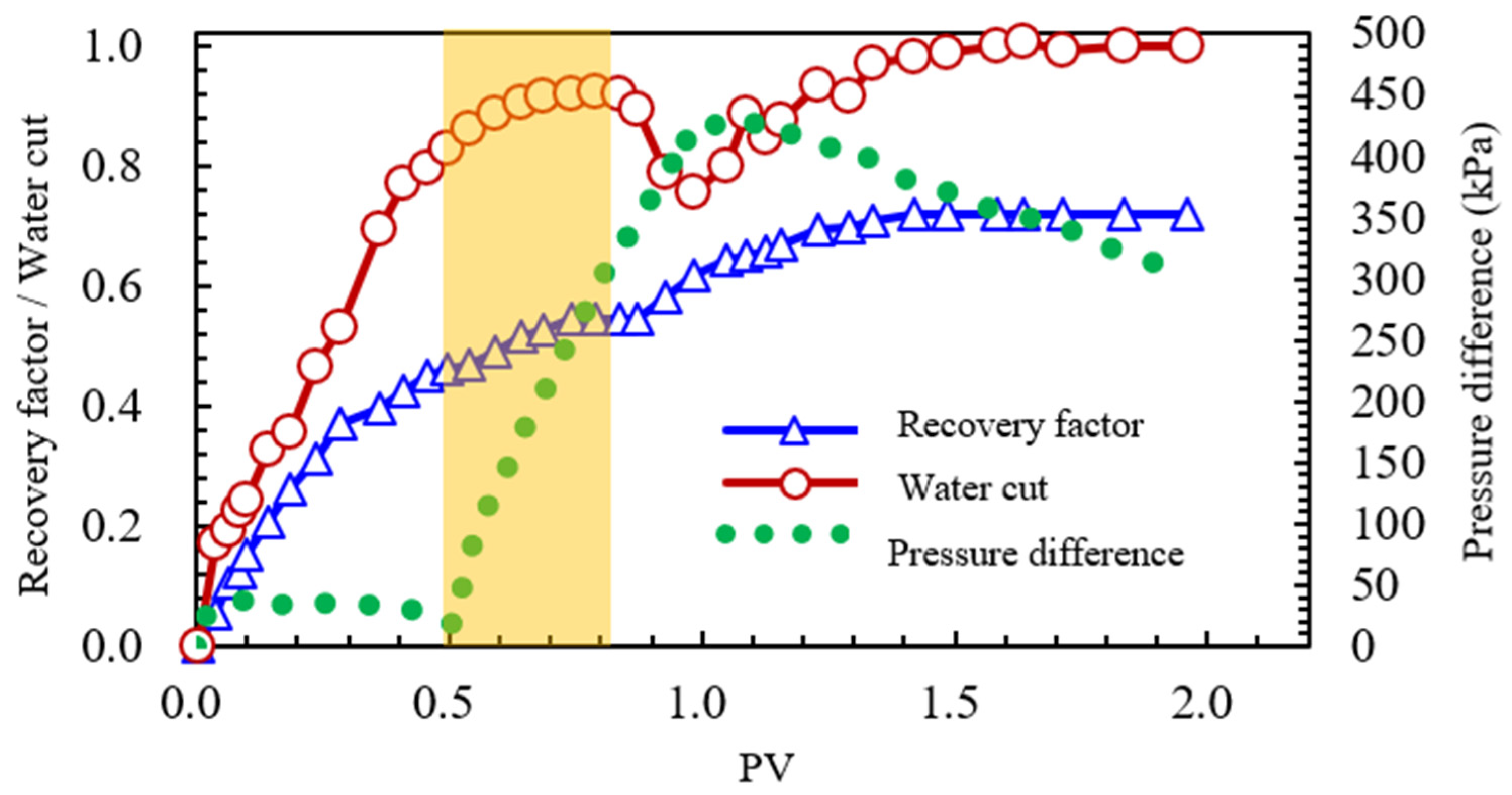
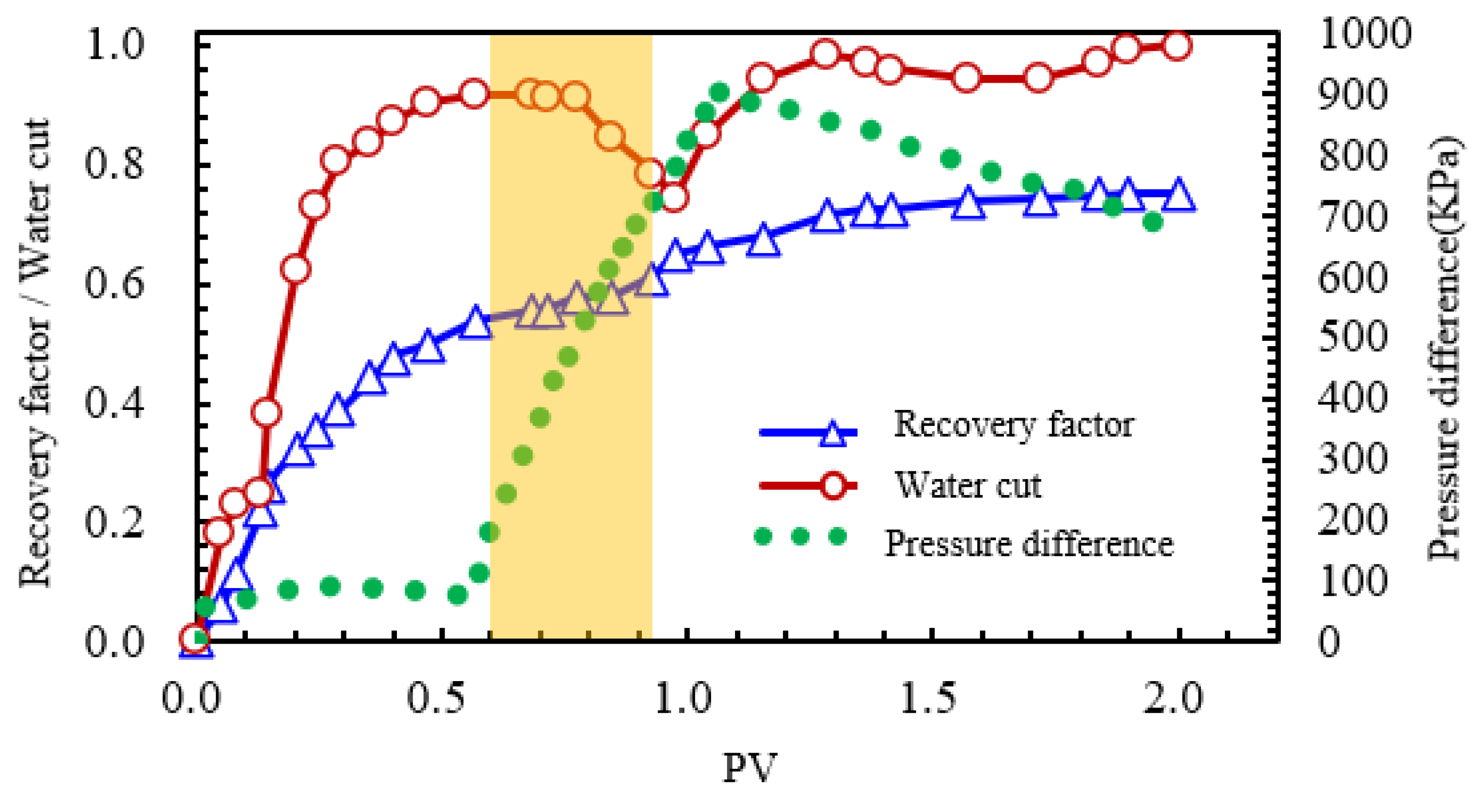
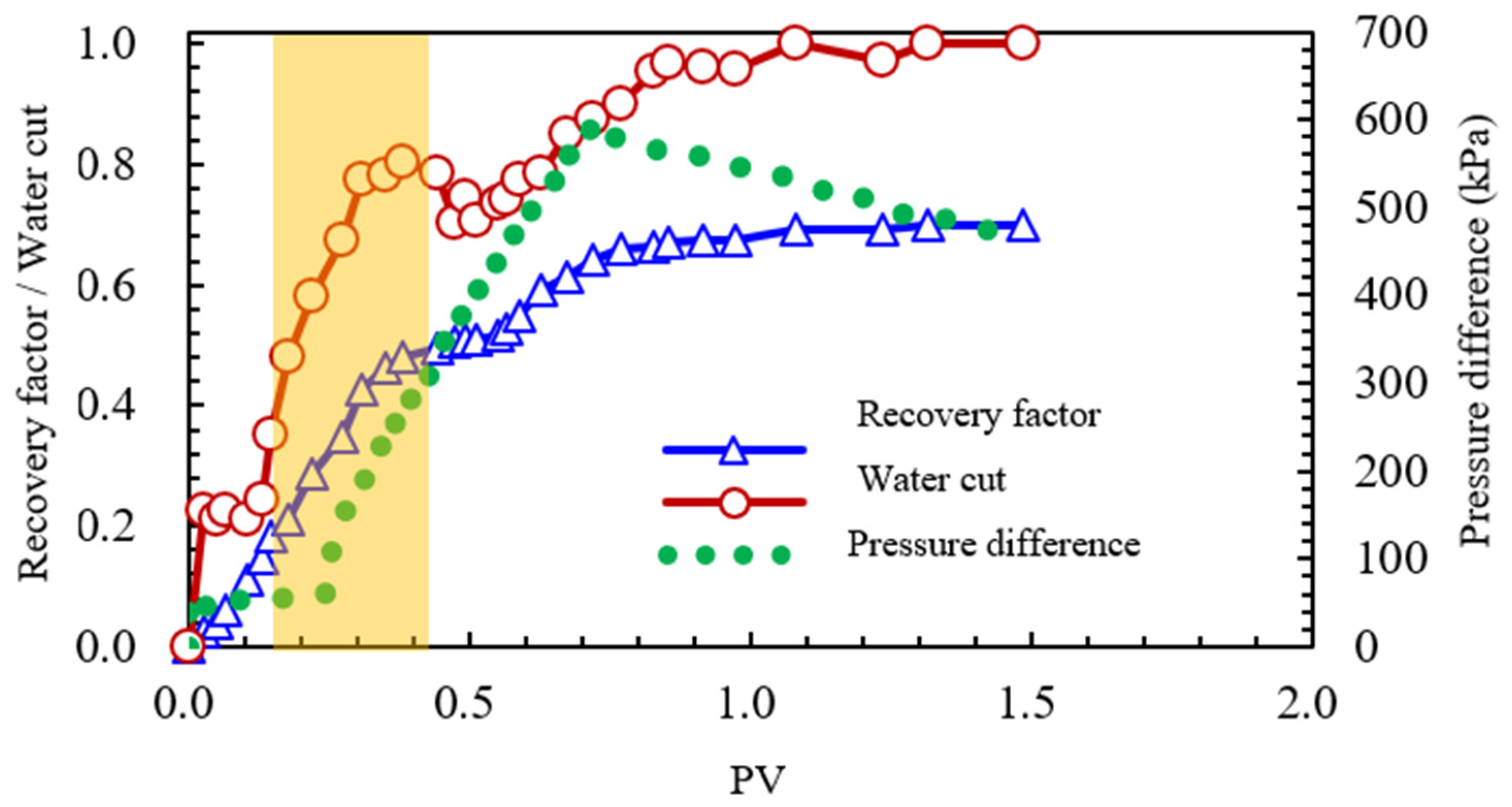
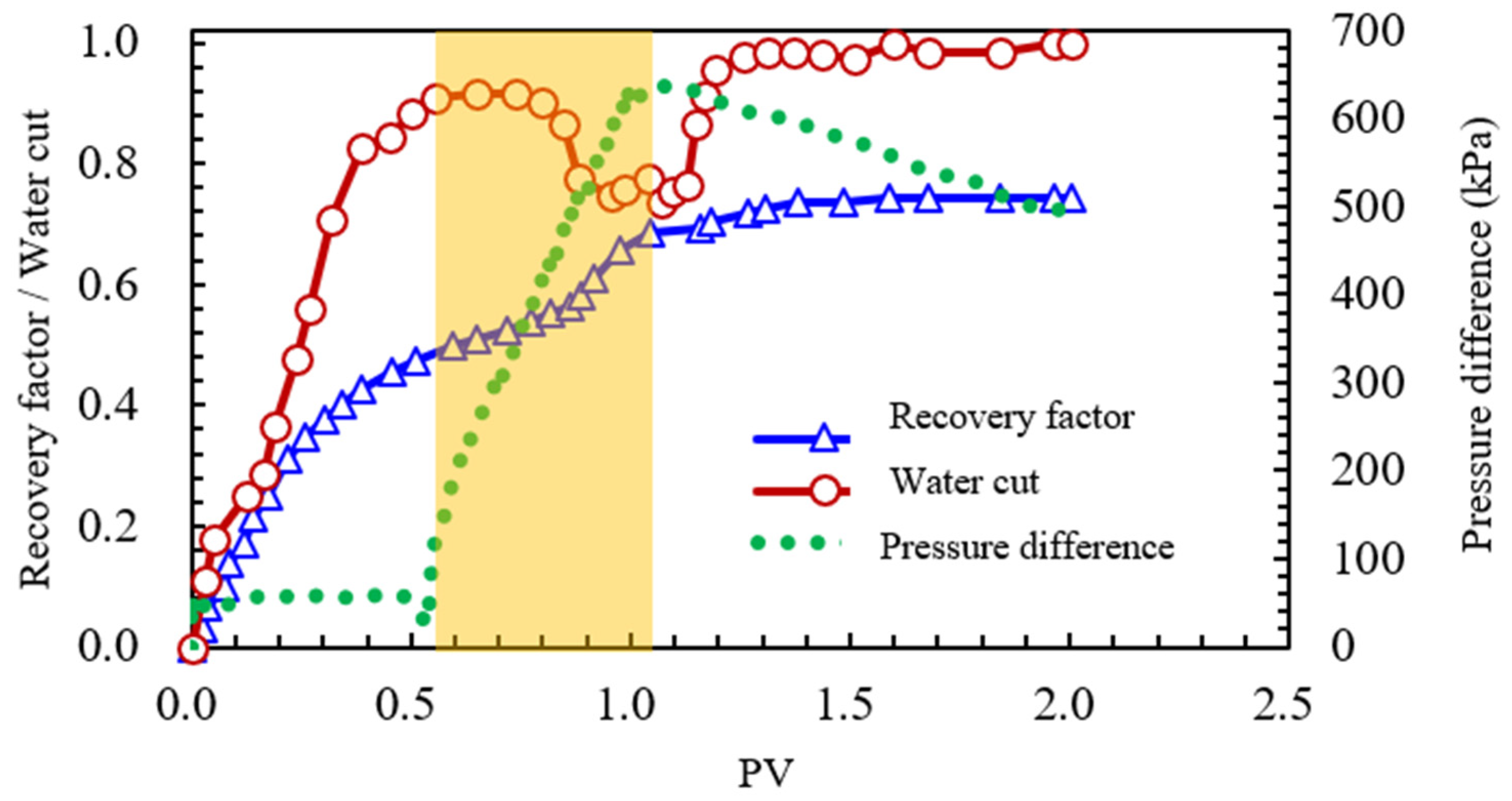
Figure 16.
Core-flooding test data after chemical treatment, with a permeability of 48.70 mD (the yellow zone indicates the chemical injection period).
Figure 16.
Core-flooding test data after chemical treatment, with a permeability of 48.70 mD (the yellow zone indicates the chemical injection period).
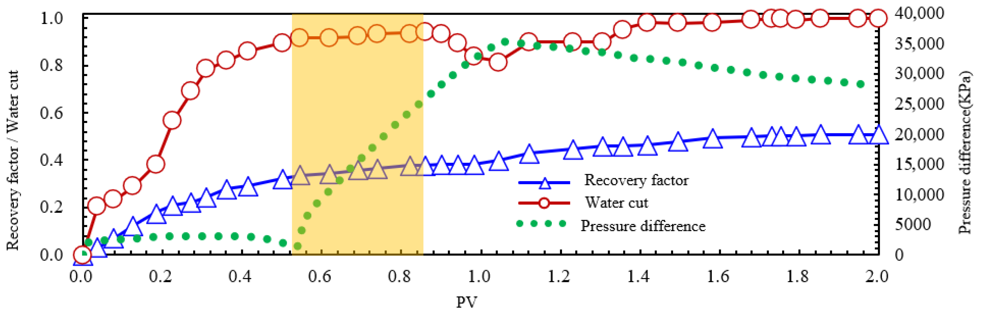
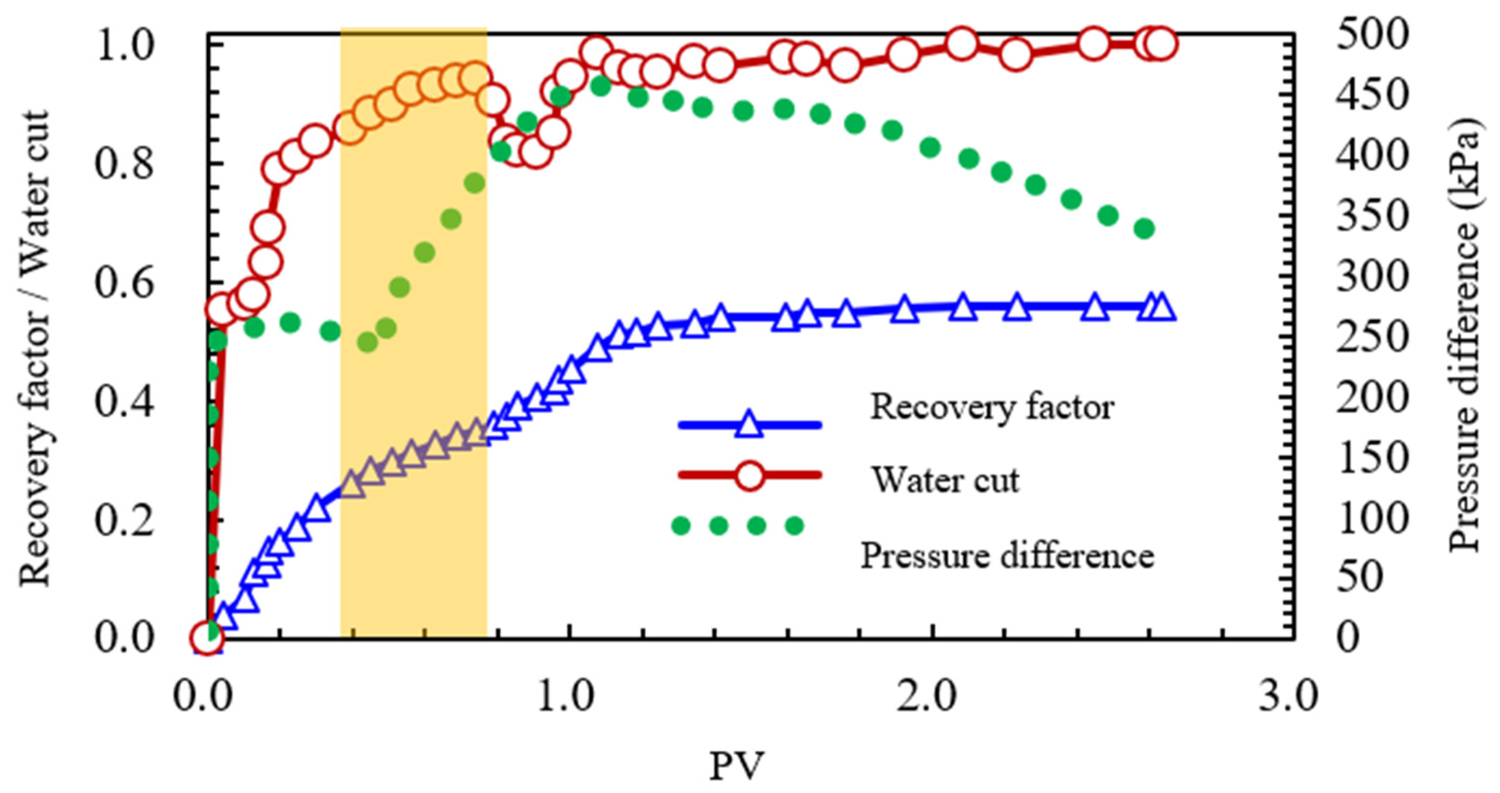
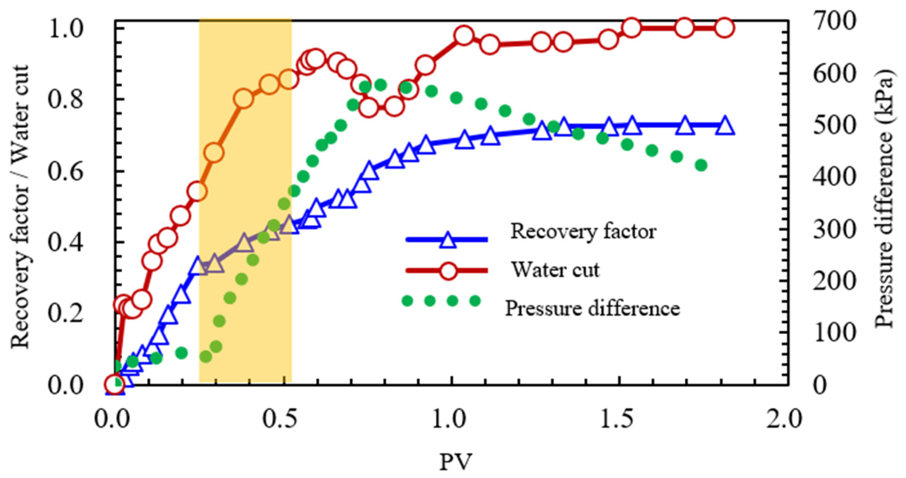
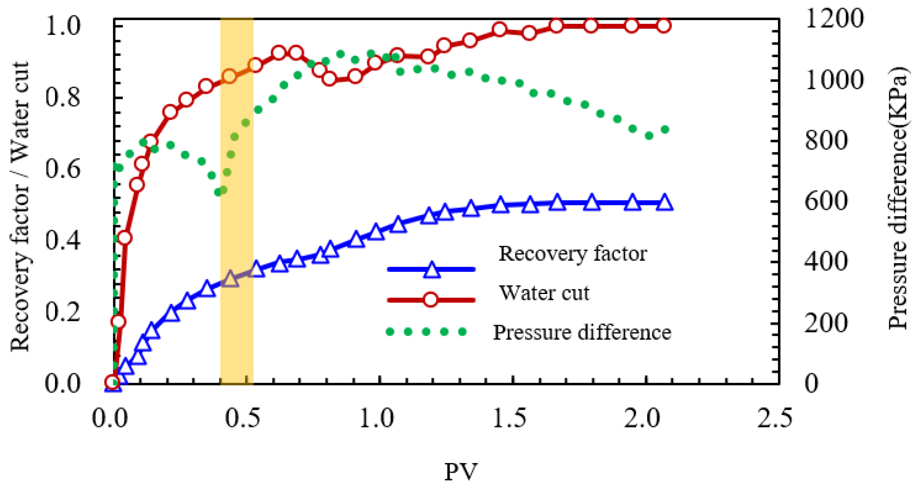
Figure 17.
Core-flooding test data after chemical treatment, with a permeability of 15.85 mD (the yellow zone indicates the chemical injection period).
Figure 17.
Core-flooding test data after chemical treatment, with a permeability of 15.85 mD (the yellow zone indicates the chemical injection period).
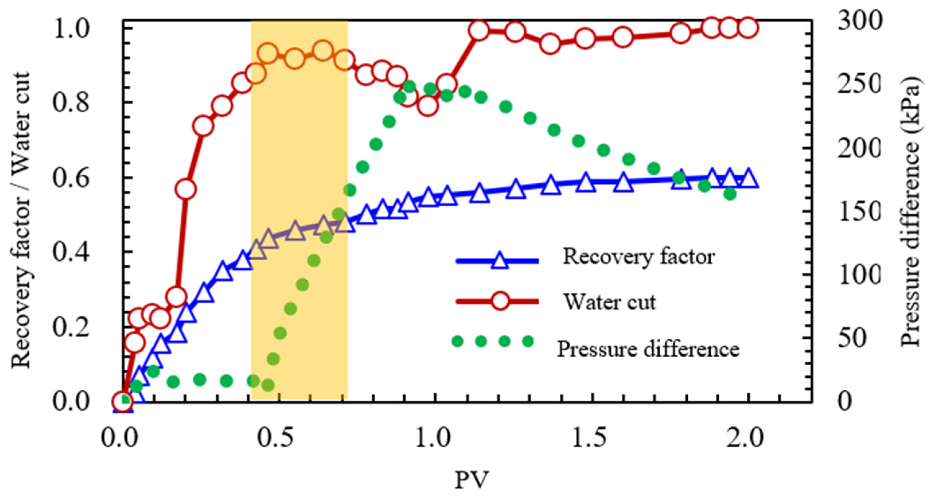
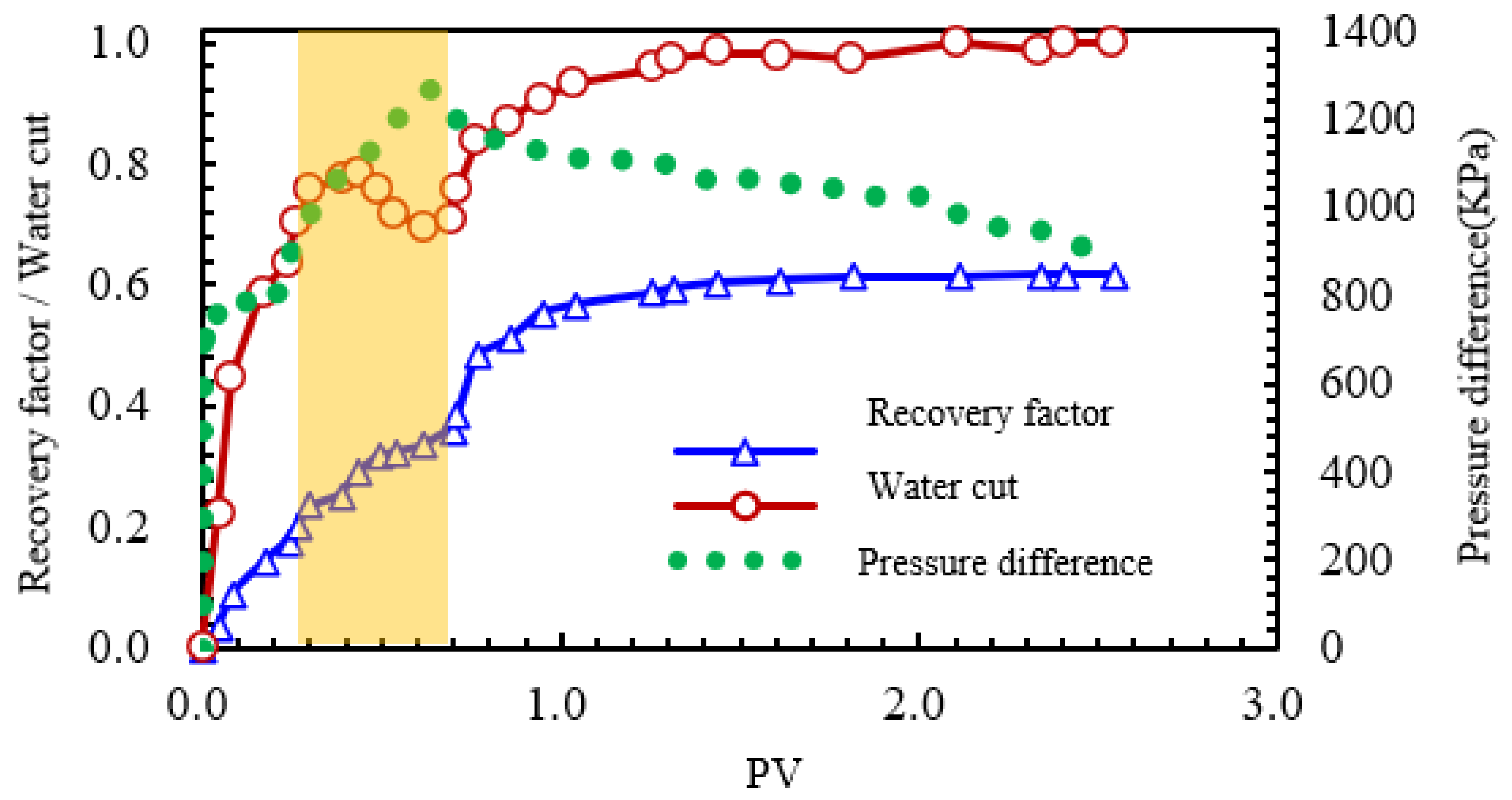
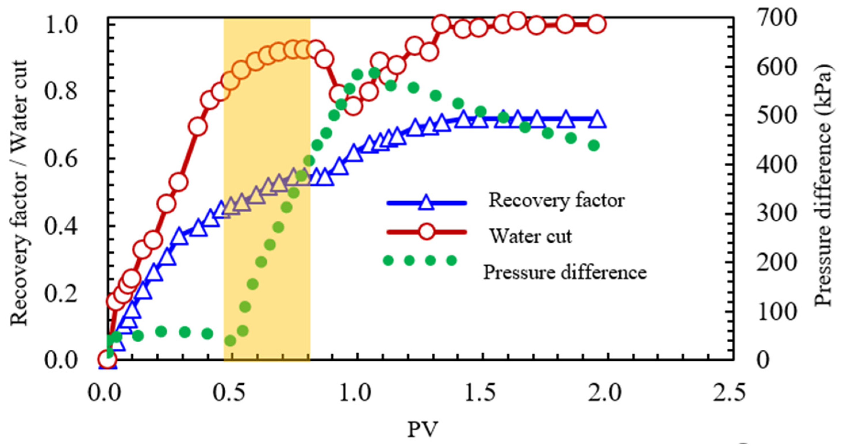
Figure 18.
Core-flooding test data after chemical treatment, with a permeability of 1.61 mD (the yellow zone indicates the chemical injection period).
Figure 18.
Core-flooding test data after chemical treatment, with a permeability of 1.61 mD (the yellow zone indicates the chemical injection period).
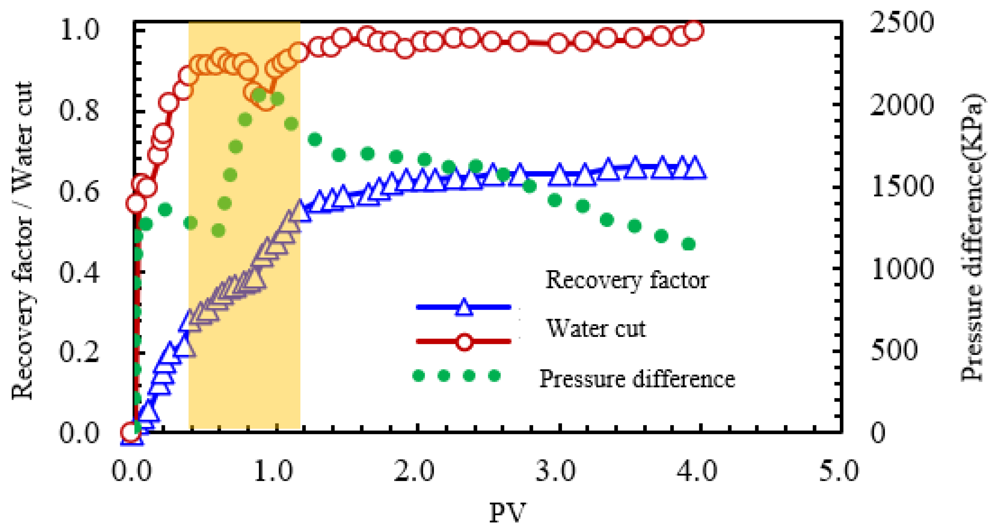
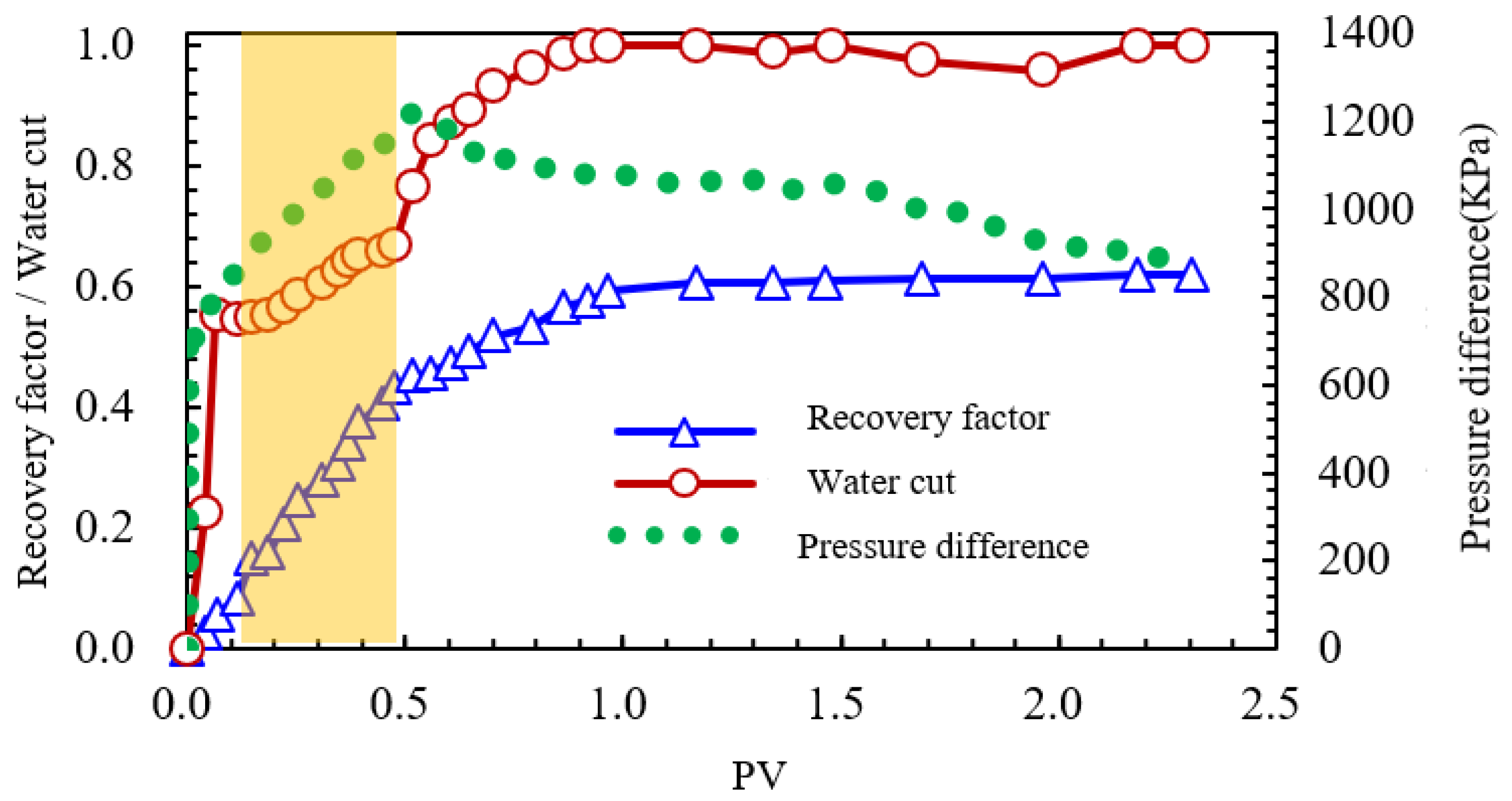
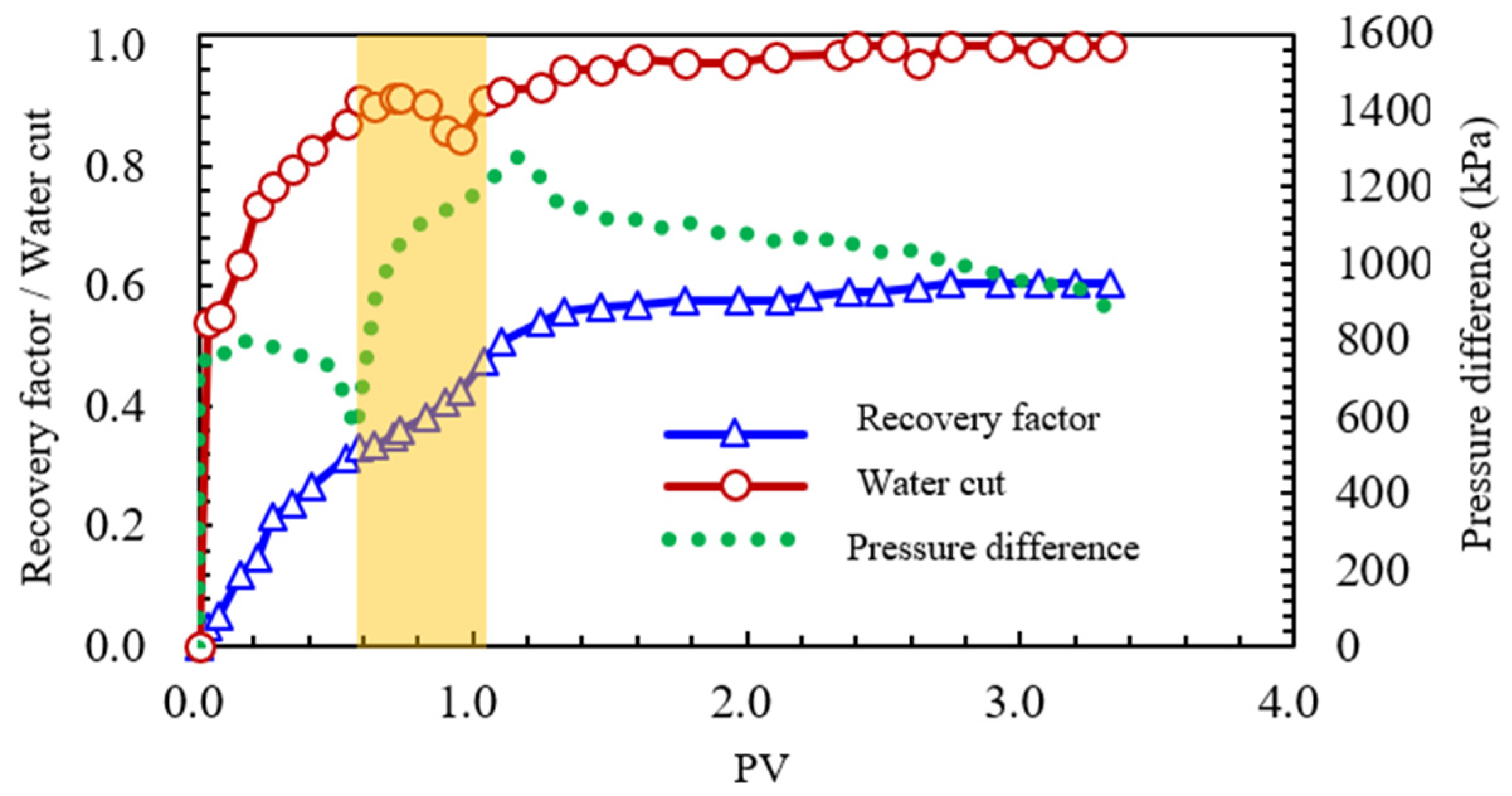
Figure 19.
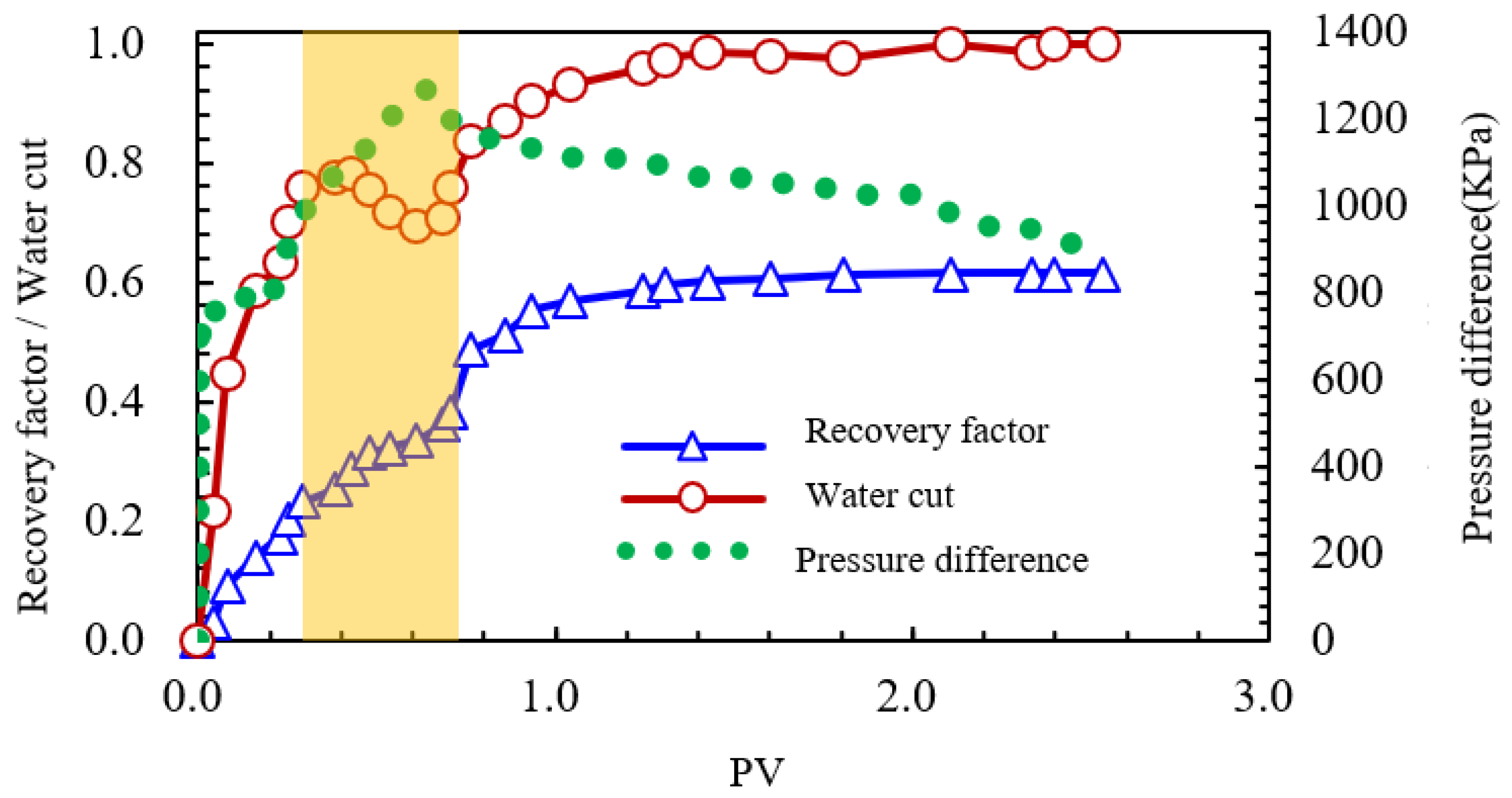
Core-flooding test data for microsphere treatment at a chemical injection rate of 0.1 cm3/min (the yellow zone indicates the chemical injection period).
Figure 19.
Core-flooding test data for microsphere treatment at a chemical injection rate of 0.1 cm3/min (the yellow zone indicates the chemical injection period).
Figure 20.
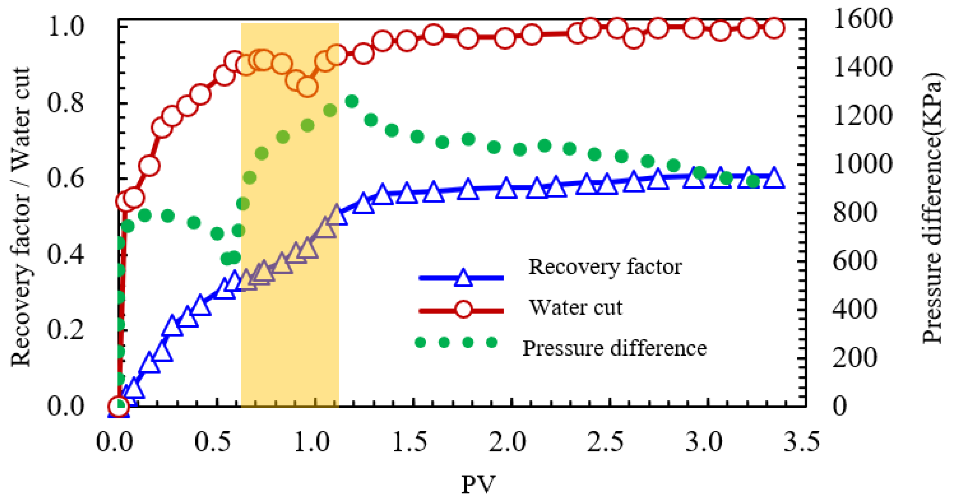
Core-flooding test data for microsphere treatment at a chemical injection rate of 0.2 cm3/min (the yellow zone indicates the chemical injection period).
Figure 20.
Core-flooding test data for microsphere treatment at a chemical injection rate of 0.2 cm3/min (the yellow zone indicates the chemical injection period).
Figure 21.
Core-flooding test data for microsphere treatment at a chemical injection rate of 0.4 cm3/min (the yellow zone indicates the chemical injection period).
Figure 21.
Core-flooding test data for microsphere treatment at a chemical injection rate of 0.4 cm3/min (the yellow zone indicates the chemical injection period).
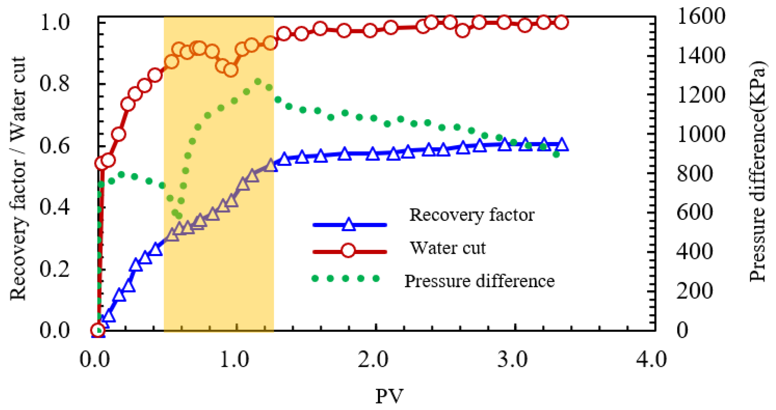
Figure 22.
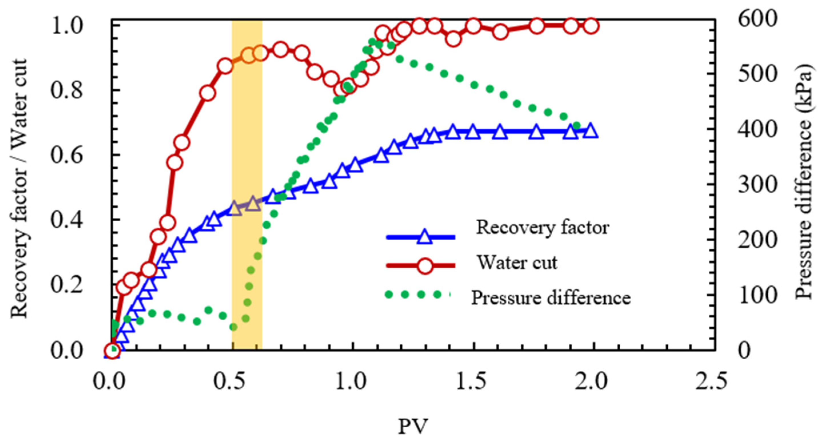
Core-flooding test data for nanoemulsion treatment at a chemical injection rate of 0.1 cm3/min (the yellow zone indicates the chemical injection period).
Figure 22.
Core-flooding test data for nanoemulsion treatment at a chemical injection rate of 0.1 cm3/min (the yellow zone indicates the chemical injection period).
Figure 23.
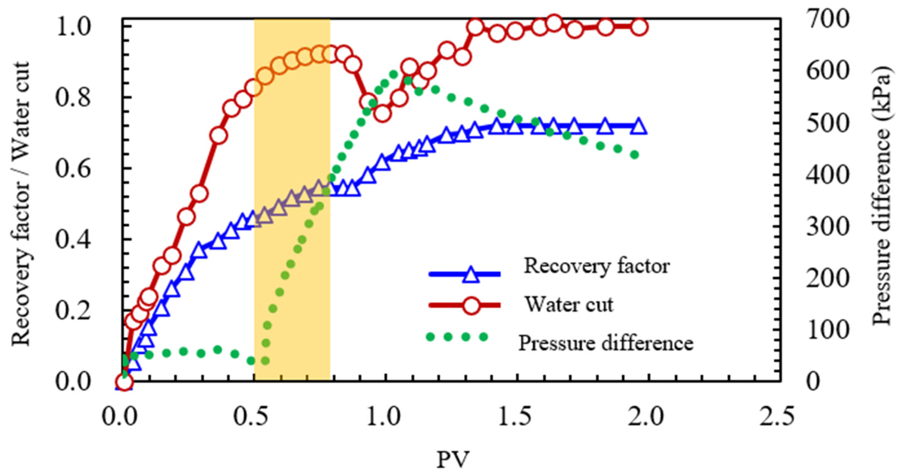
Core-flooding test data for nanoemulsion treatment at a chemical injection rate of 0.2 cm3/min (the yellow zone indicates the chemical injection period).
Figure 23.
Core-flooding test data for nanoemulsion treatment at a chemical injection rate of 0.2 cm3/min (the yellow zone indicates the chemical injection period).
Figure 24.
Core-flooding test data for nanoemulsion treatment at a chemical injection rate of 0.4 cm3/min (the yellow zone indicates the chemical injection period).
Figure 24.
Core-flooding test data for nanoemulsion treatment at a chemical injection rate of 0.4 cm3/min (the yellow zone indicates the chemical injection period).
Figure 25.
Core-flooding test data for microsphere treatment, with chemical injection initiated at 0.5 water flooding face (the yellow zone indicates the chemical injection period).
Figure 25.
Core-flooding test data for microsphere treatment, with chemical injection initiated at 0.5 water flooding face (the yellow zone indicates the chemical injection period).
Figure 26.
Core-flooding test data for microsphere treatment, with chemical injection initiated at 0.7 water flooding face (the yellow zone indicates the chemical injection period).
Figure 26.
Core-flooding test data for microsphere treatment, with chemical injection initiated at 0.7 water flooding face (the yellow zone indicates the chemical injection period).
Figure 27.
Core-flooding test data for microsphere treatment, with chemical injection initiated at 0.9 water flooding face (the yellow zone indicates the chemical injection period).
Figure 27.
Core-flooding test data for microsphere treatment, with chemical injection initiated at 0.9 water flooding face (the yellow zone indicates the chemical injection period).
Figure 28.
Core-flooding test data for nanoemulsion treatment, with chemical injection initiated at 0.5 water flooding face (the yellow zone indicates the chemical injection period).
Figure 28.
Core-flooding test data for nanoemulsion treatment, with chemical injection initiated at 0.5 water flooding face (the yellow zone indicates the chemical injection period).
Figure 29.
Core-flooding test data for nanoemulsion treatment, with chemical injection initiated at 0.7 water flooding face (the yellow zone indicates the chemical injection period).
Figure 29.
Core-flooding test data for nanoemulsion treatment, with chemical injection initiated at 0.7 water flooding face (the yellow zone indicates the chemical injection period).
Figure 30.
Core-flooding test for nanoemulsion treatment, with chemical injection initiated at 0.9 water flooding face (the yellow zone indicates the chemical injection period).
Figure 30.
Core-flooding test for nanoemulsion treatment, with chemical injection initiated at 0.9 water flooding face (the yellow zone indicates the chemical injection period).
Figure 31.
Core-flooding test data for microsphere treatment at a chemical injection volume of 0.1 PV (the yellow zone indicates the chemical injection period).
Figure 31.
Core-flooding test data for microsphere treatment at a chemical injection volume of 0.1 PV (the yellow zone indicates the chemical injection period).
Figure 32.
Core-flooding test data for microsphere treatment at a chemical injection volume of 0.3 PV (the yellow zone indicates the chemical injection period).
Figure 32.
Core-flooding test data for microsphere treatment at a chemical injection volume of 0.3 PV (the yellow zone indicates the chemical injection period).
Figure 33.
Core-flooding test data for microsphere treatment at a chemical injection volume of 0.5 PV (the yellow zone indicates the chemical injection period).
Figure 33.
Core-flooding test data for microsphere treatment at a chemical injection volume of 0.5 PV (the yellow zone indicates the chemical injection period).
Figure 34.
Core-flooding test for nanoemulsion treatment at a chemical injection volume of 0.1 PV (the yellow zone indicates the chemical injection period).
Figure 34.
Core-flooding test for nanoemulsion treatment at a chemical injection volume of 0.1 PV (the yellow zone indicates the chemical injection period).
Figure 35.
Core-flooding test for nanoemulsion treatment at a chemical injection volume of 0.3 PV (the yellow zone indicates the chemical injection period).
Figure 35.
Core-flooding test for nanoemulsion treatment at a chemical injection volume of 0.3 PV (the yellow zone indicates the chemical injection period).
Figure 36.
Core-flooding test for nanoemulsion treatment at a chemical injection volume of 0.5 PV (the yellow zone indicates the chemical injection period).
Figure 36.
Core-flooding test for nanoemulsion treatment at a chemical injection volume of 0.5 PV (the yellow zone indicates the chemical injection period).
Figure 37.
Core-flooding test data for microsphere treatment conducted on multiple core samples under various composite conditions. (a) 15.85 + 8.70 mD; (b) 15.85 + 1.61 mD, (the yellow zone indicates the chemical injection period).
Figure 37.
Core-flooding test data for microsphere treatment conducted on multiple core samples under various composite conditions. (a) 15.85 + 8.70 mD; (b) 15.85 + 1.61 mD, (the yellow zone indicates the chemical injection period).
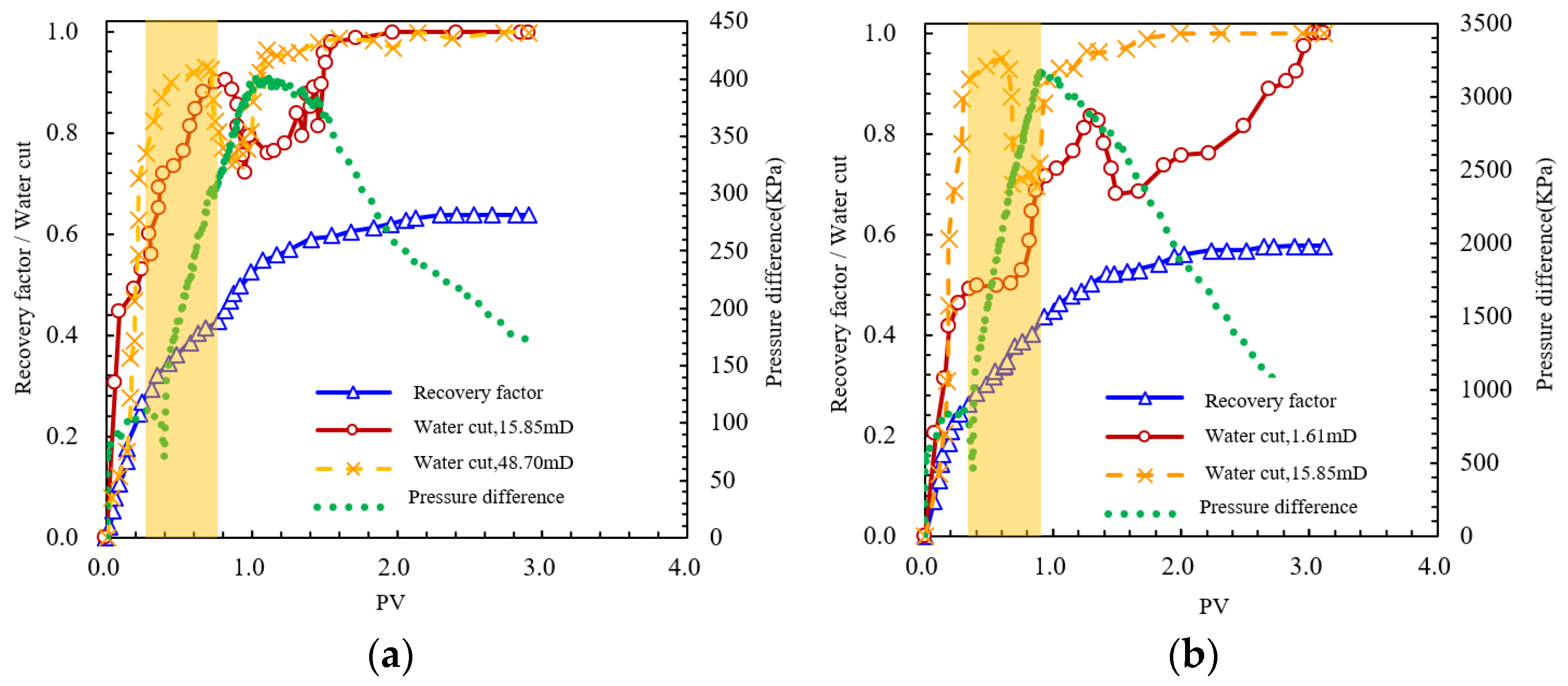
Figure 38.
Core-flooding test data for nanoemulsion treatment conducted on multiple core samples under various composite conditions, (a) 15.85 + 8.70 mD; (b) 15.85 + 1.61 mD. (the yellow zone indicates the chemical injection period).
Figure 38.
Core-flooding test data for nanoemulsion treatment conducted on multiple core samples under various composite conditions, (a) 15.85 + 8.70 mD; (b) 15.85 + 1.61 mD. (the yellow zone indicates the chemical injection period).
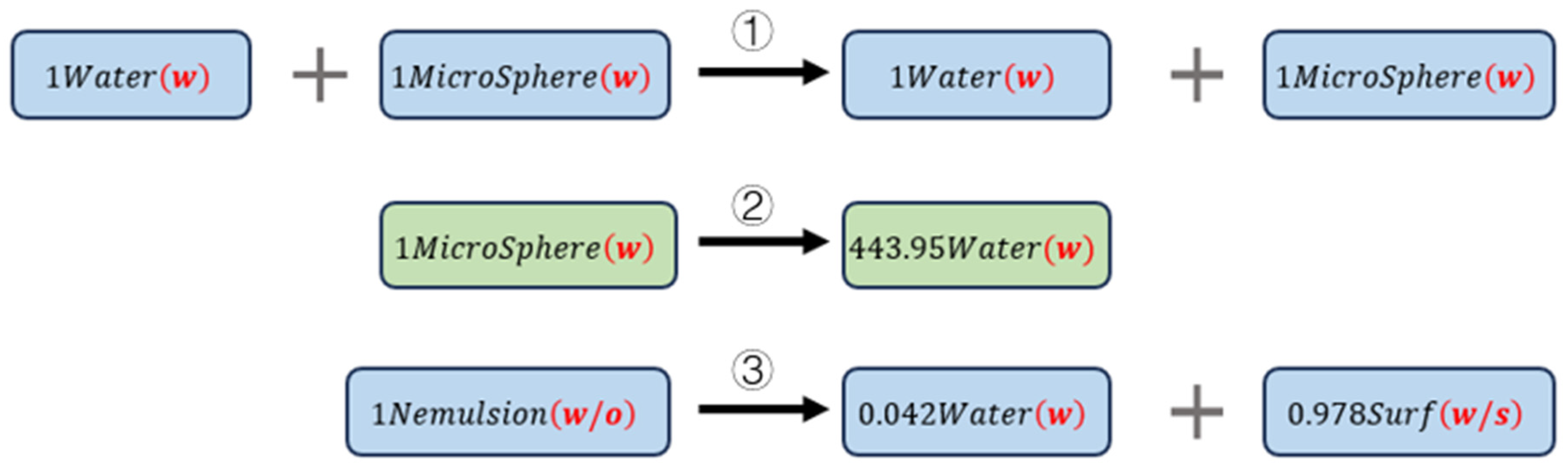
Figure 39.
Equivalent reactions between pseudo components, ① Hydration and Swelling of Microspheres; ② Destabilization of Microspheres; ③ Adsorption and Phase Separation of Nanoemulsion.
Figure 39.
Equivalent reactions between pseudo components, ① Hydration and Swelling of Microspheres; ② Destabilization of Microspheres; ③ Adsorption and Phase Separation of Nanoemulsion.
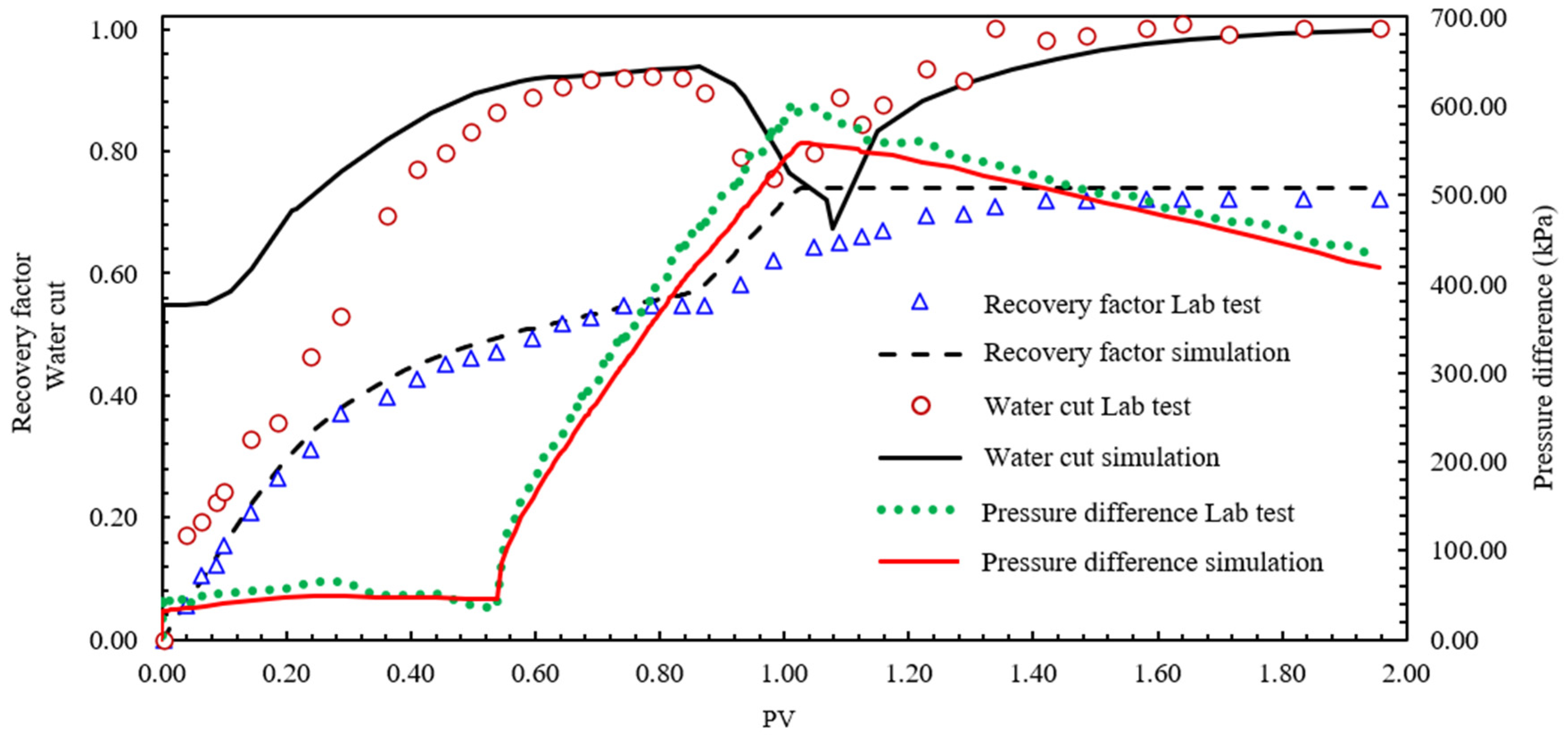
Figure 40.
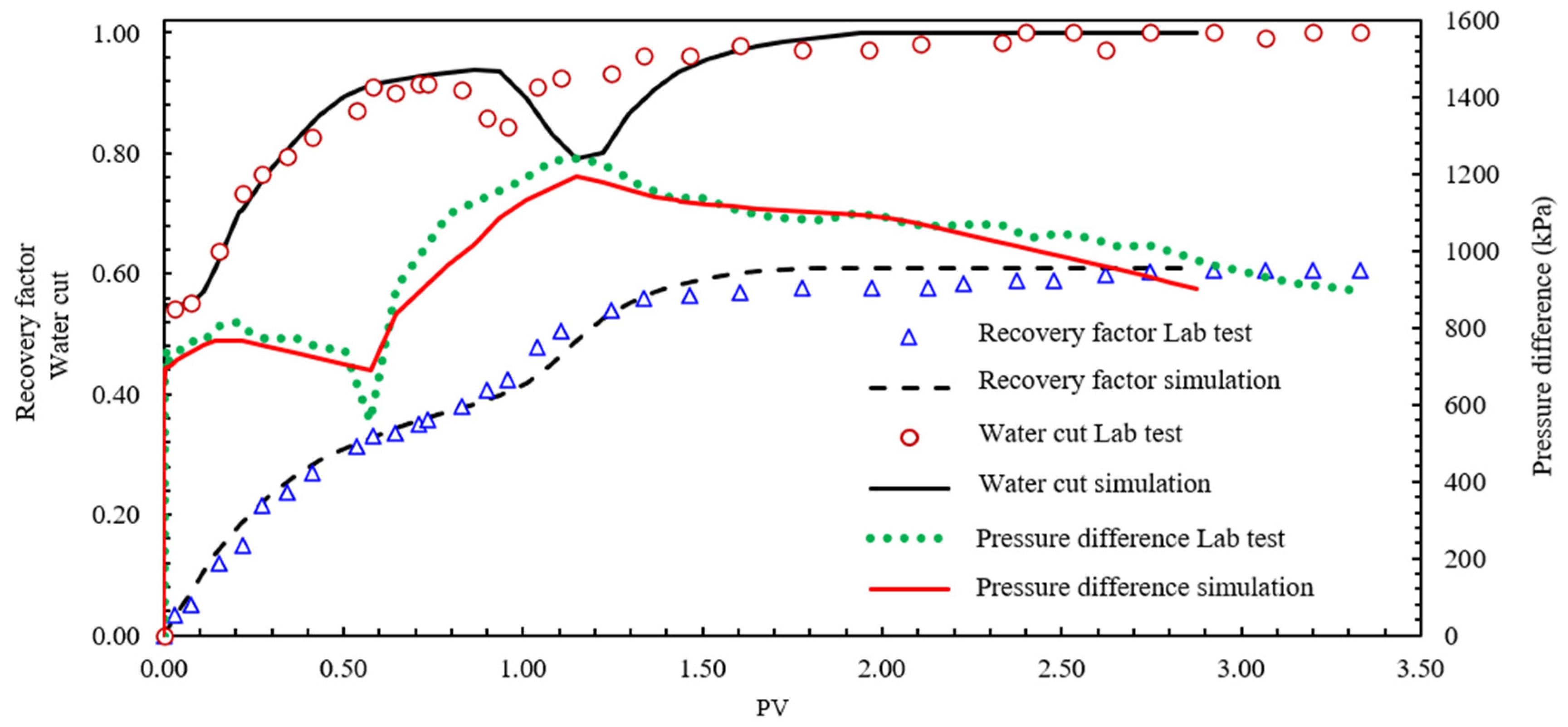
Comparison of microsphere simulation results with core-flood data.
Figure 40.
Comparison of microsphere simulation results with core-flood data.
Figure 41.
Comparison of nanoemulsion simulation results with core-flood data.
Figure 41.
Comparison of nanoemulsion simulation results with core-flood data.
Figure 42.
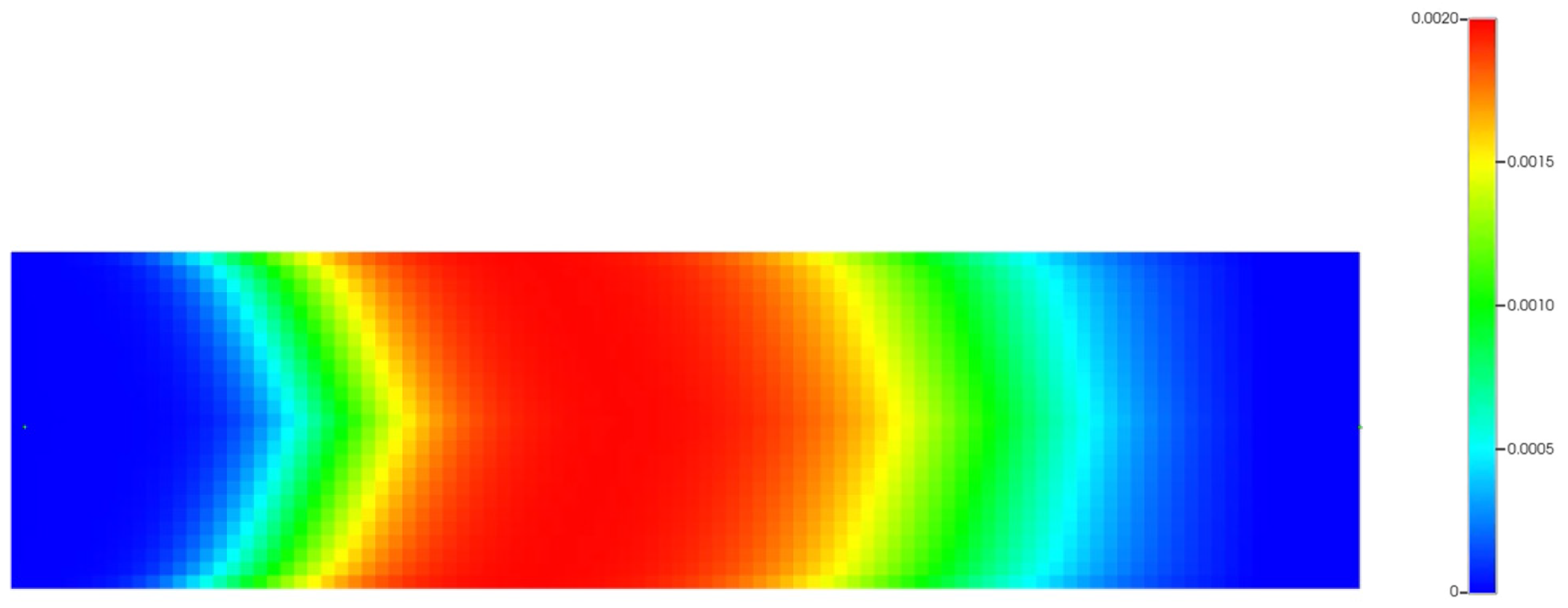
Pre-expansion microsphere component distribution (the flow direction from the injection end to the production end is from left to right).
Figure 42.
Pre-expansion microsphere component distribution (the flow direction from the injection end to the production end is from left to right).
Figure 43.
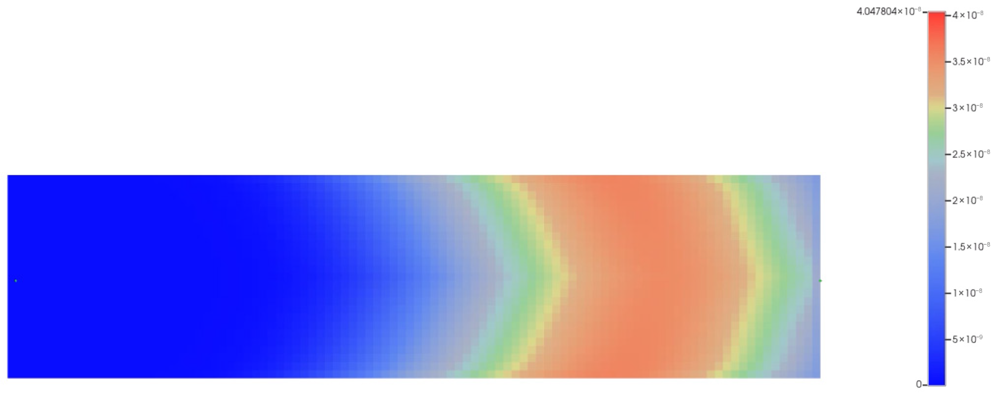
Post-expansion microsphere component distribution (the flow direction from the injection end to the production end is from left to right).
Figure 43.
Post-expansion microsphere component distribution (the flow direction from the injection end to the production end is from left to right).
Figure 44.
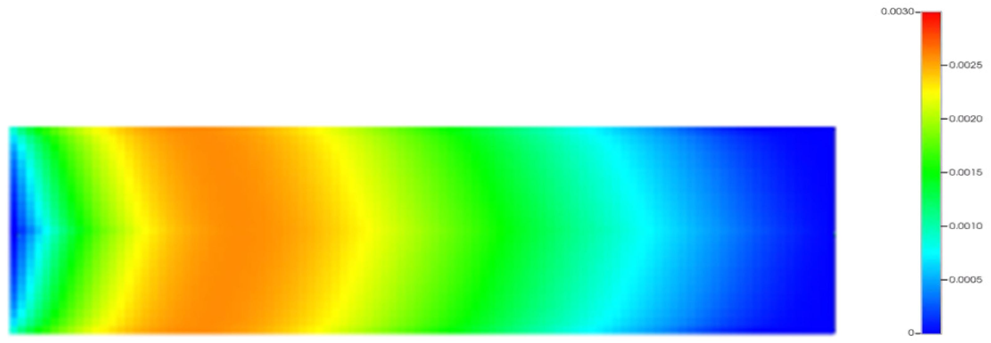
Component distribution of nanoemulsion during migration (the flow direction from the injection end to the production end is from left to right).
Figure 44.
Component distribution of nanoemulsion during migration (the flow direction from the injection end to the production end is from left to right).
Figure 45.
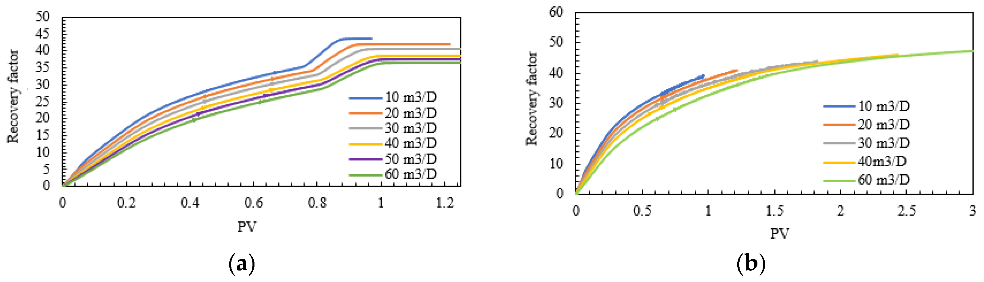
Oil-recovery curves at different injection rates. (a) microsphere; (b) nanoemulsion.
Figure 45.
Oil-recovery curves at different injection rates. (a) microsphere; (b) nanoemulsion.
Figure 46.
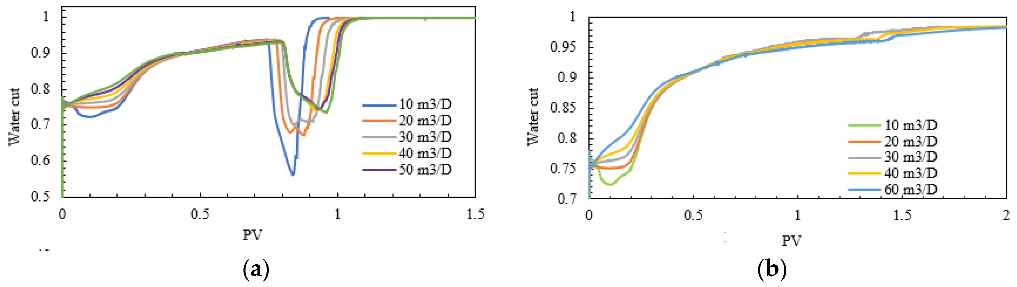
Water-cut curves at different injection rates. (a) microsphere; (b) nanoemulsion.
Figure 46.
Water-cut curves at different injection rates. (a) microsphere; (b) nanoemulsion.
Figure 47.
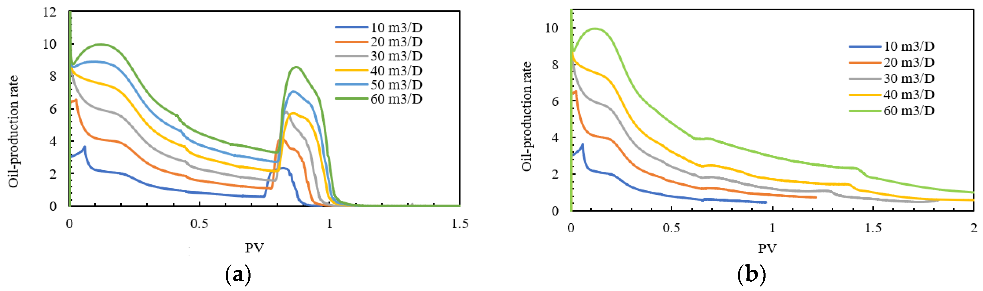
Oil-production rate curves for microsphere and nanoemulsion at different injection rates. (a) microsphere; (b) nanoemulsion.
Figure 47.
Oil-production rate curves for microsphere and nanoemulsion at different injection rates. (a) microsphere; (b) nanoemulsion.
Figure 48.
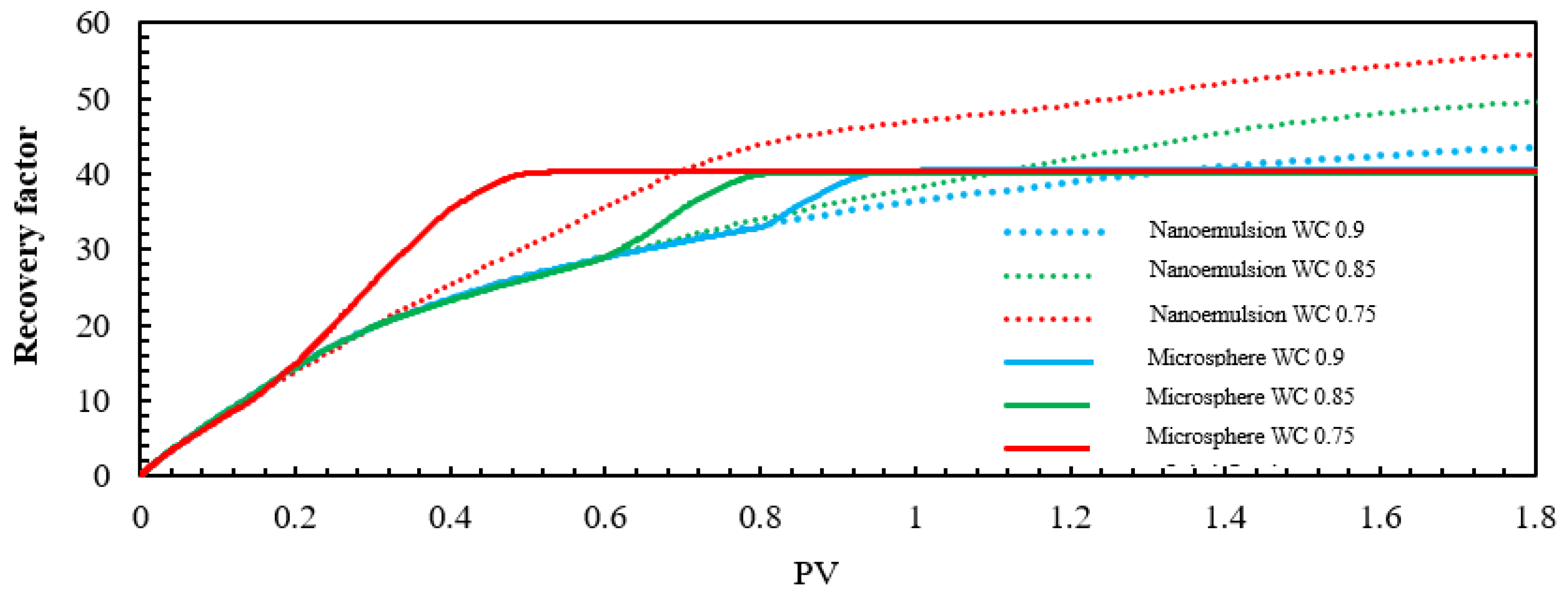
Oil-recovery curves under different injection timing (WC0.9, WC0.85, WC0.75) scenarios for microsphere and nanoemulsion.
Figure 48.
Oil-recovery curves under different injection timing (WC0.9, WC0.85, WC0.75) scenarios for microsphere and nanoemulsion.
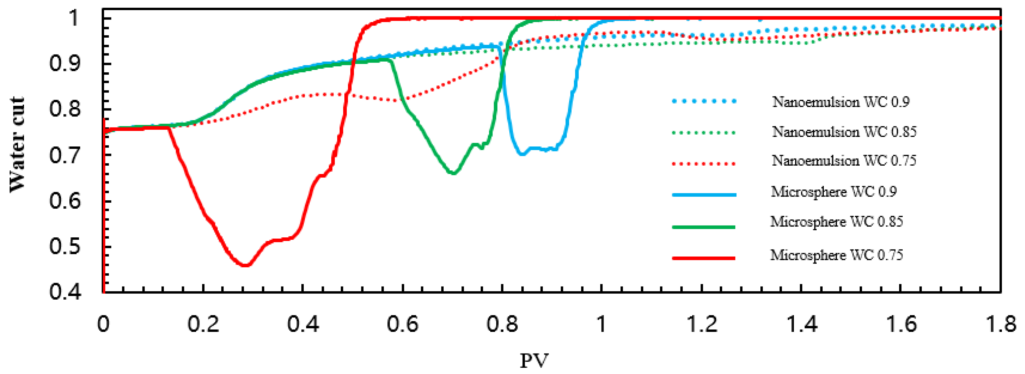
Figure 49.
Water-cut curves under different injection timing (WC0.9, WC0.85, WC0.75) scenarios for microsphere and nanoemulsion.
Figure 49.
Water-cut curves under different injection timing (WC0.9, WC0.85, WC0.75) scenarios for microsphere and nanoemulsion.
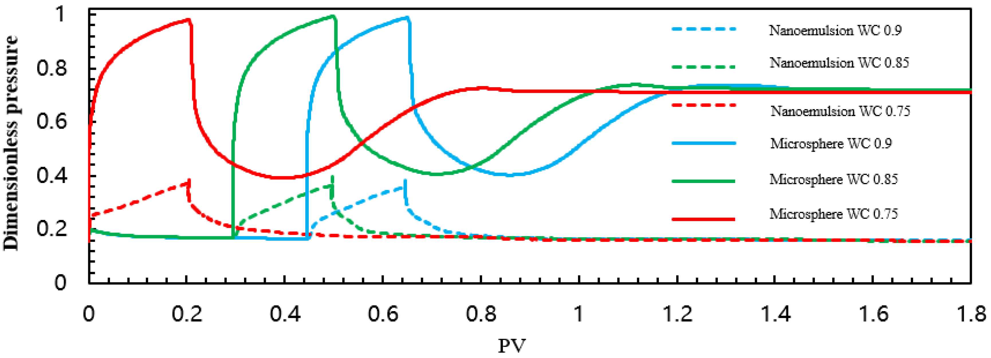
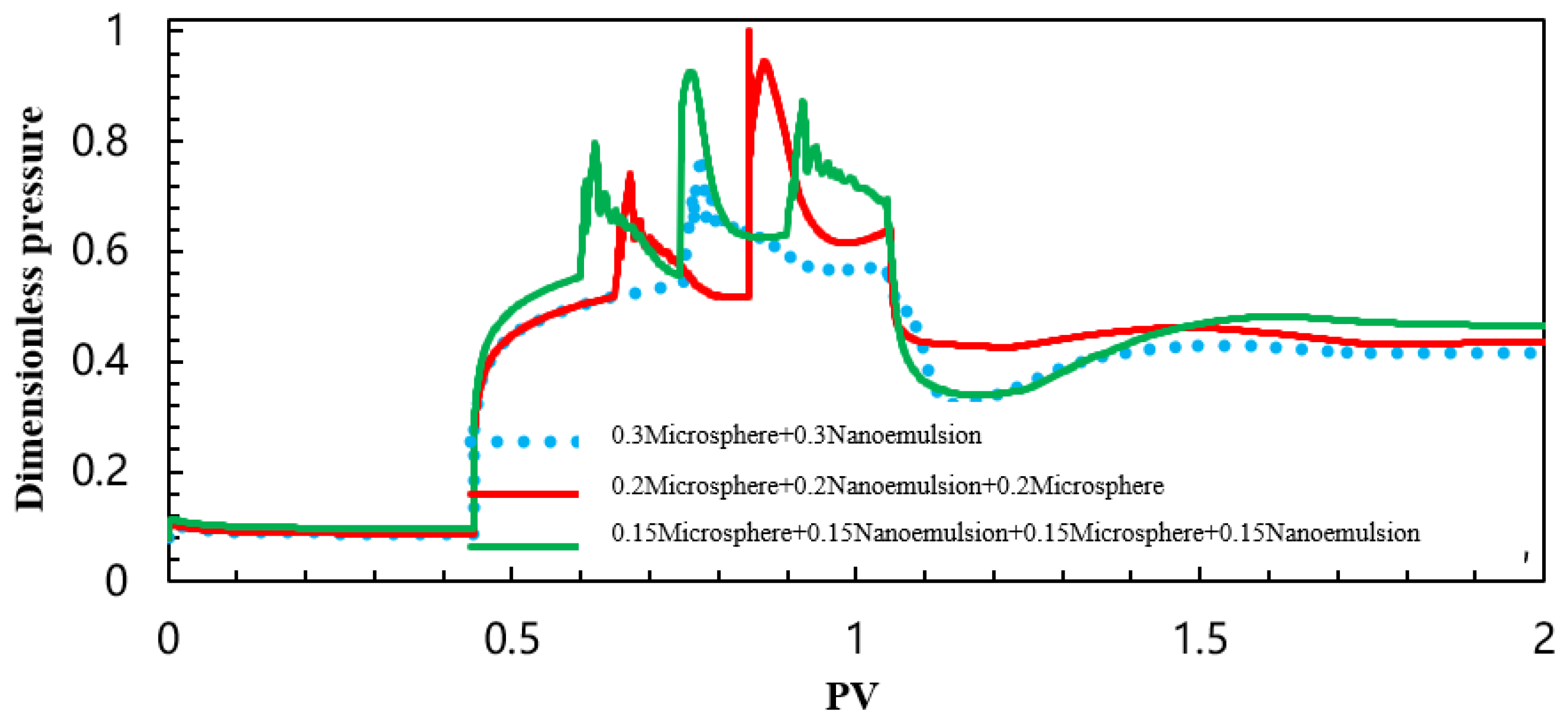
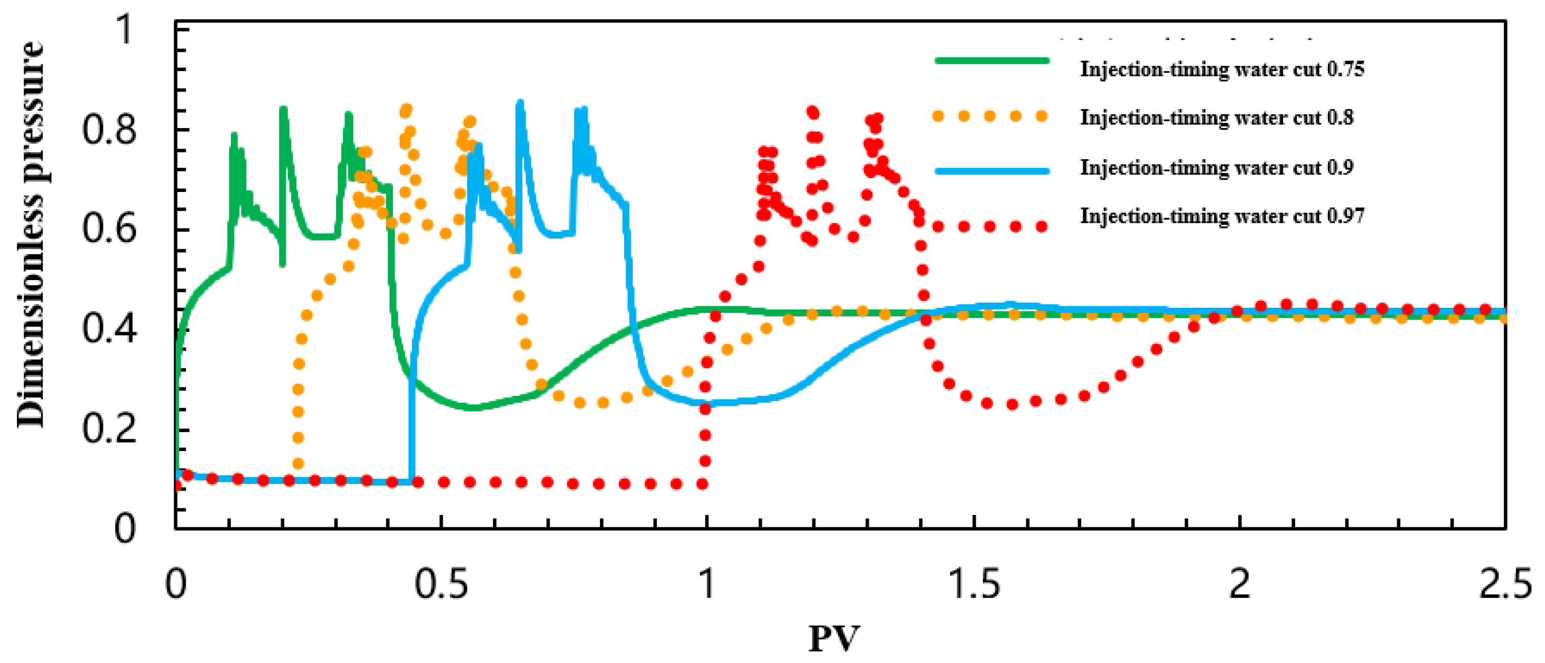
Figure 50.
Dimensionless pressure curves under different injection timing (WC0.9, WC0.85, WC0.75) scenarios for microsphere and nanoemulsion.
Figure 50.
Dimensionless pressure curves under different injection timing (WC0.9, WC0.85, WC0.75) scenarios for microsphere and nanoemulsion.
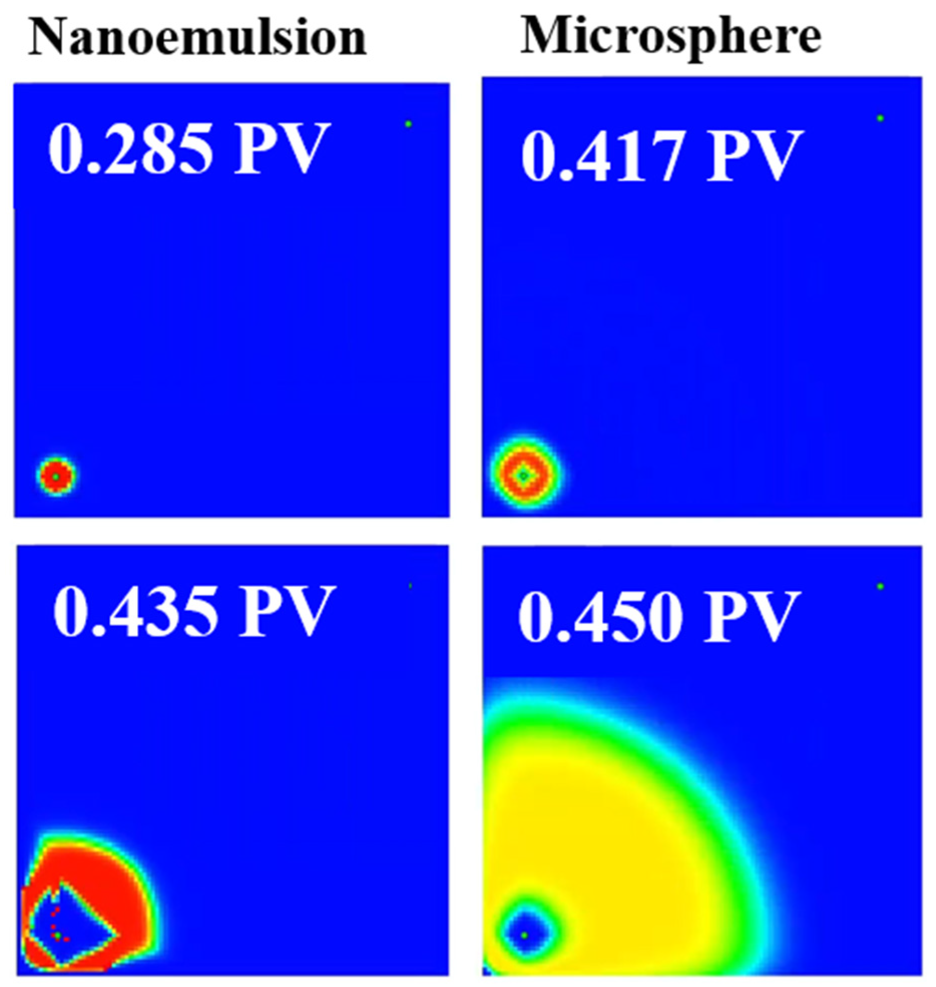
Figure 51.
Component distribution under different injection volumes of microsphere and nanoemulsion (injection timing = 0.8) (the colormap represents the concentration of microspheres or nanoemulsion, with red indicating a higher concentration).
Figure 51.
Component distribution under different injection volumes of microsphere and nanoemulsion (injection timing = 0.8) (the colormap represents the concentration of microspheres or nanoemulsion, with red indicating a higher concentration).
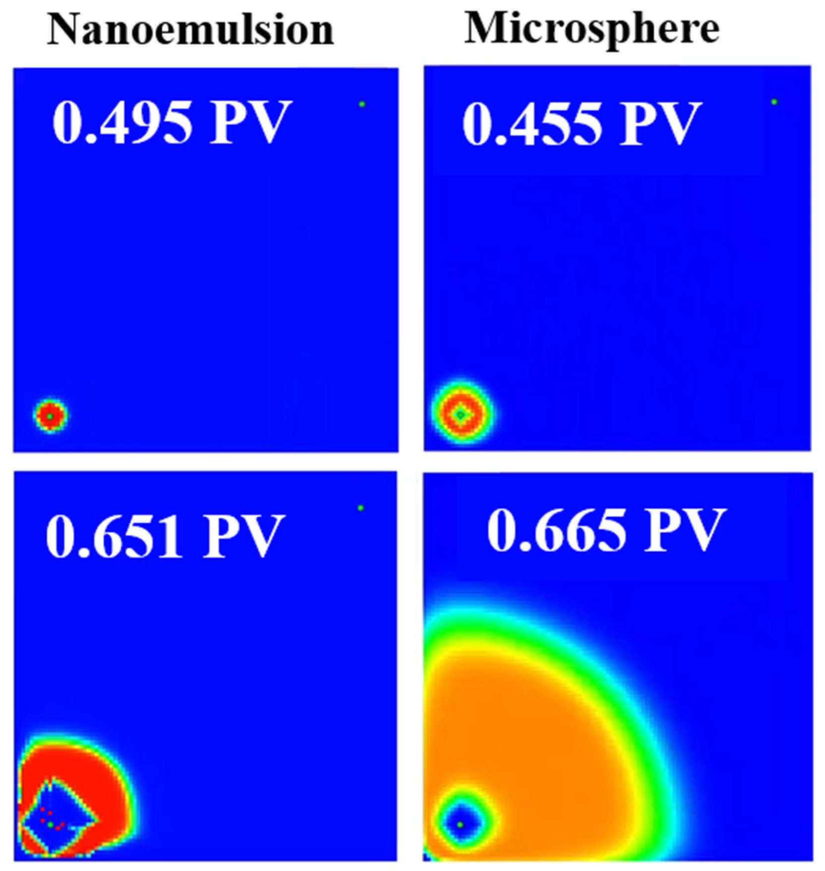
Figure 52.
Component distribution under different injection volumes of microsphere and nanoemulsion (injection timing = 0.9) (the colormap represents the concentration of microspheres or nanoemulsion, with red indicating a higher concentration).
Figure 52.
Component distribution under different injection volumes of microsphere and nanoemulsion (injection timing = 0.9) (the colormap represents the concentration of microspheres or nanoemulsion, with red indicating a higher concentration).
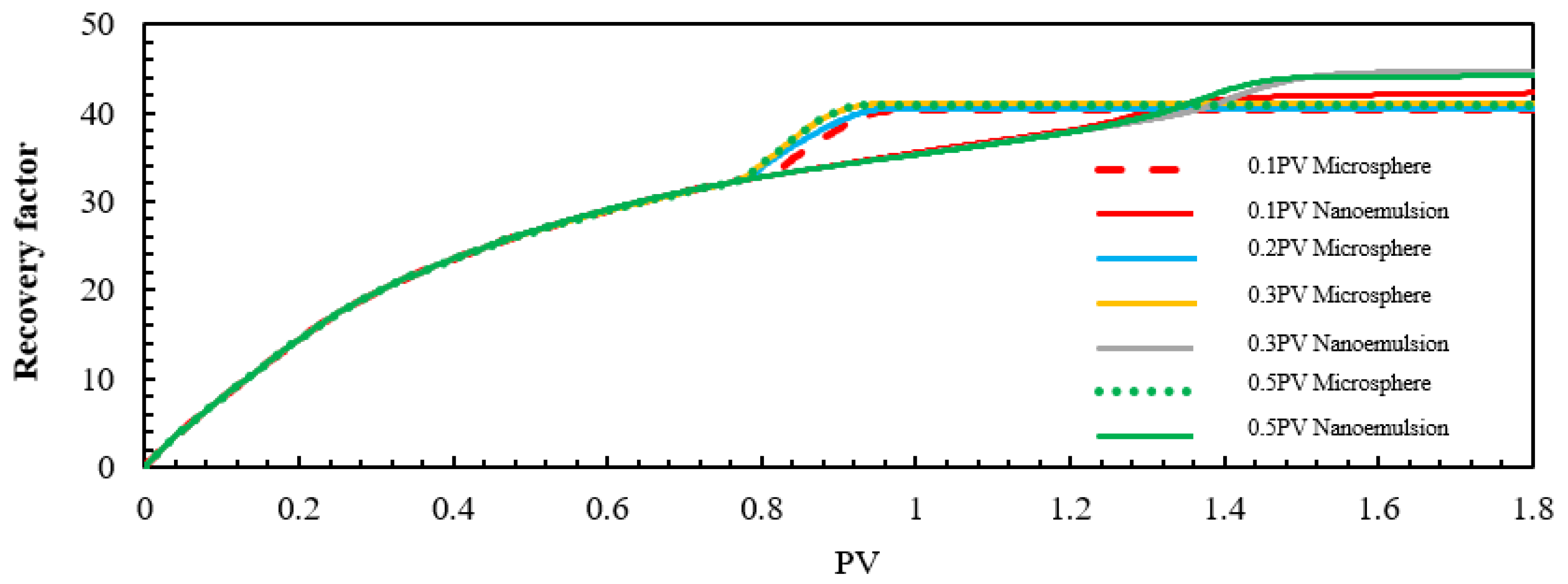
Figure 53.
Oil-recovery curves under different injection volumes (0.1 PV, 0.2 PV 0.3 PV, 0.5 PV) of microsphere and nanoemulsion.
Figure 53.
Oil-recovery curves under different injection volumes (0.1 PV, 0.2 PV 0.3 PV, 0.5 PV) of microsphere and nanoemulsion.
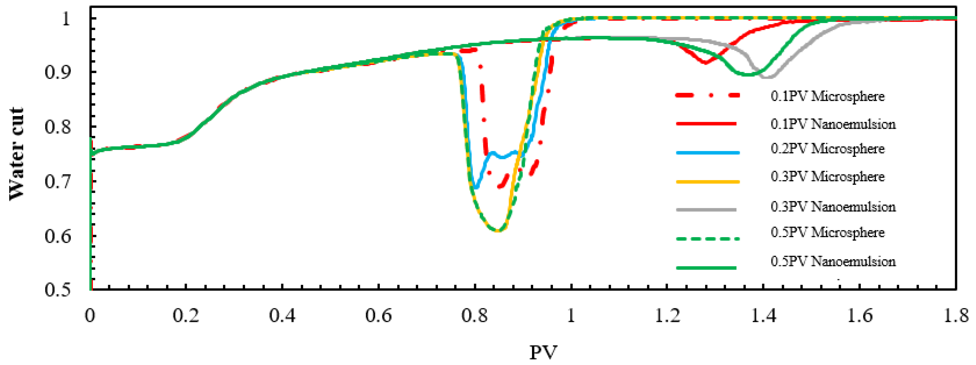
Figure 54.
Water-cut curves under different injection volumes (0.1 PV, 0.2 PV 0.3 PV, 0.5 PV) of microsphere and nanoemulsion.
Figure 54.
Water-cut curves under different injection volumes (0.1 PV, 0.2 PV 0.3 PV, 0.5 PV) of microsphere and nanoemulsion.
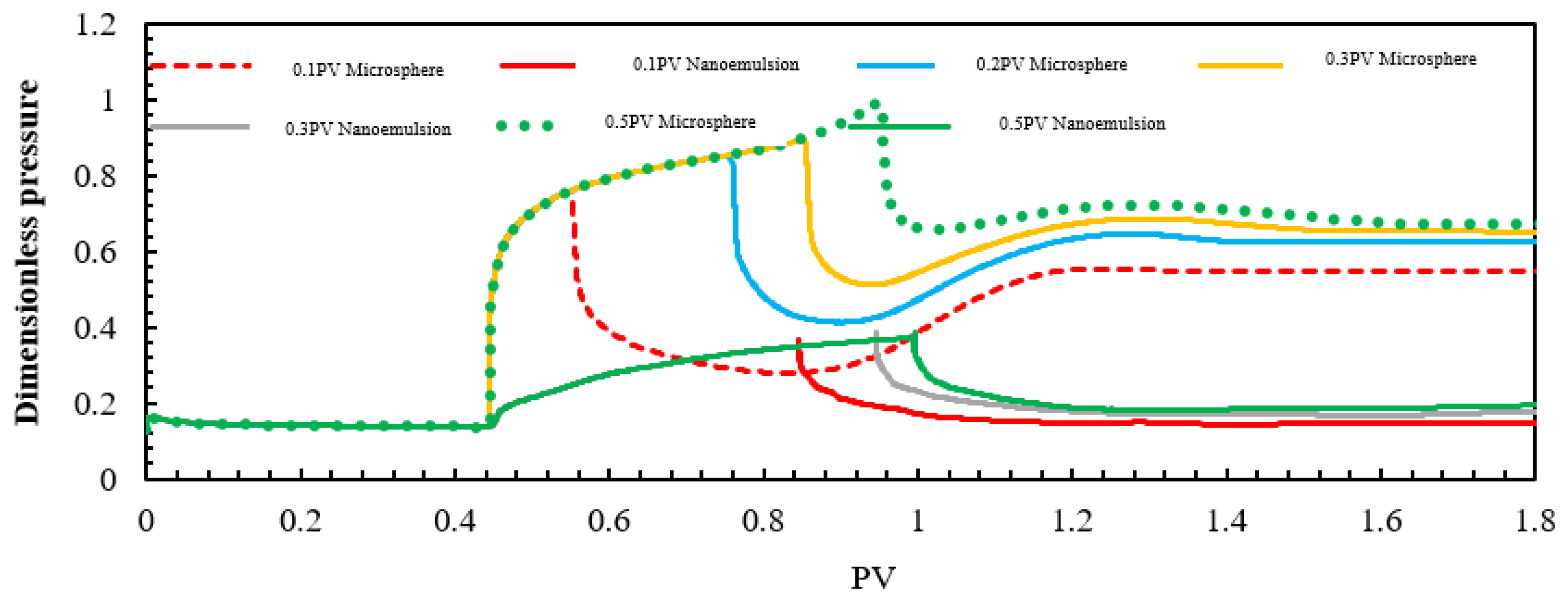
Figure 55.
Dimensionless-pressure curves under different injection volumes (0.1 PV, 0.2 PV 0.3 PV, 0.5 PV) of microsphere and nanoemulsion.
Figure 55.
Dimensionless-pressure curves under different injection volumes (0.1 PV, 0.2 PV 0.3 PV, 0.5 PV) of microsphere and nanoemulsion.
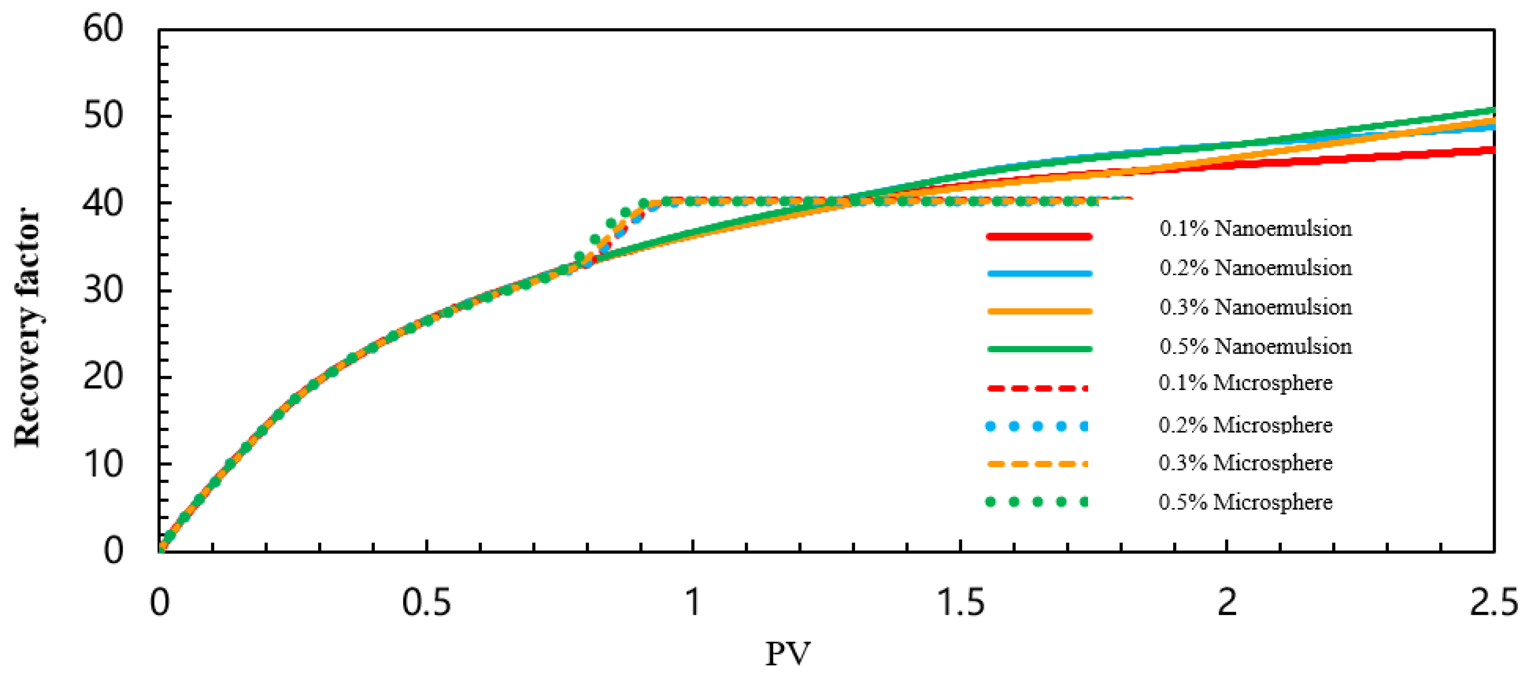
Figure 56.
Oil-recovery curves at different concentrations of microsphere and nanoemulsion.
Figure 56.
Oil-recovery curves at different concentrations of microsphere and nanoemulsion.
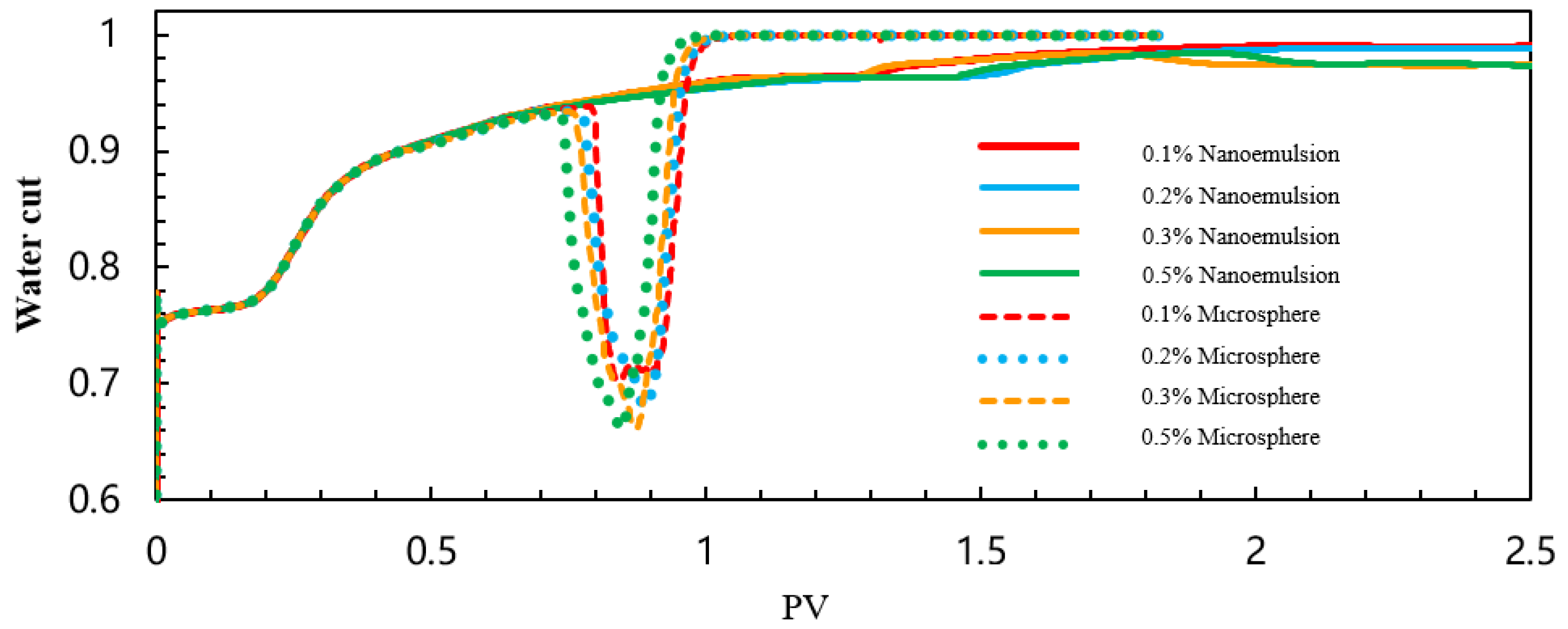
Figure 57.
Water-cut curves at different concentrations of microsphere and nanoemulsion.
Figure 57.
Water-cut curves at different concentrations of microsphere and nanoemulsion.
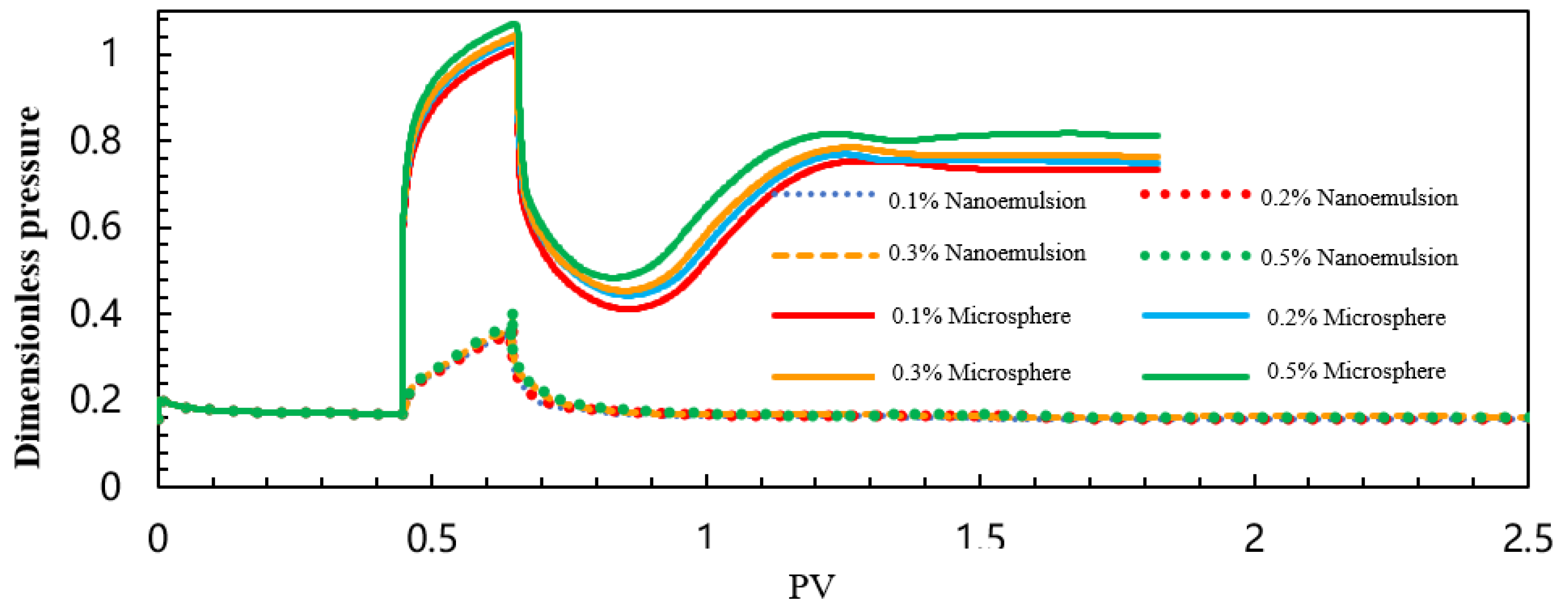
Figure 58.
Dimensionless-pressure curves at different concentrations of microsphere and nanoemulsion.
Figure 58.
Dimensionless-pressure curves at different concentrations of microsphere and nanoemulsion.
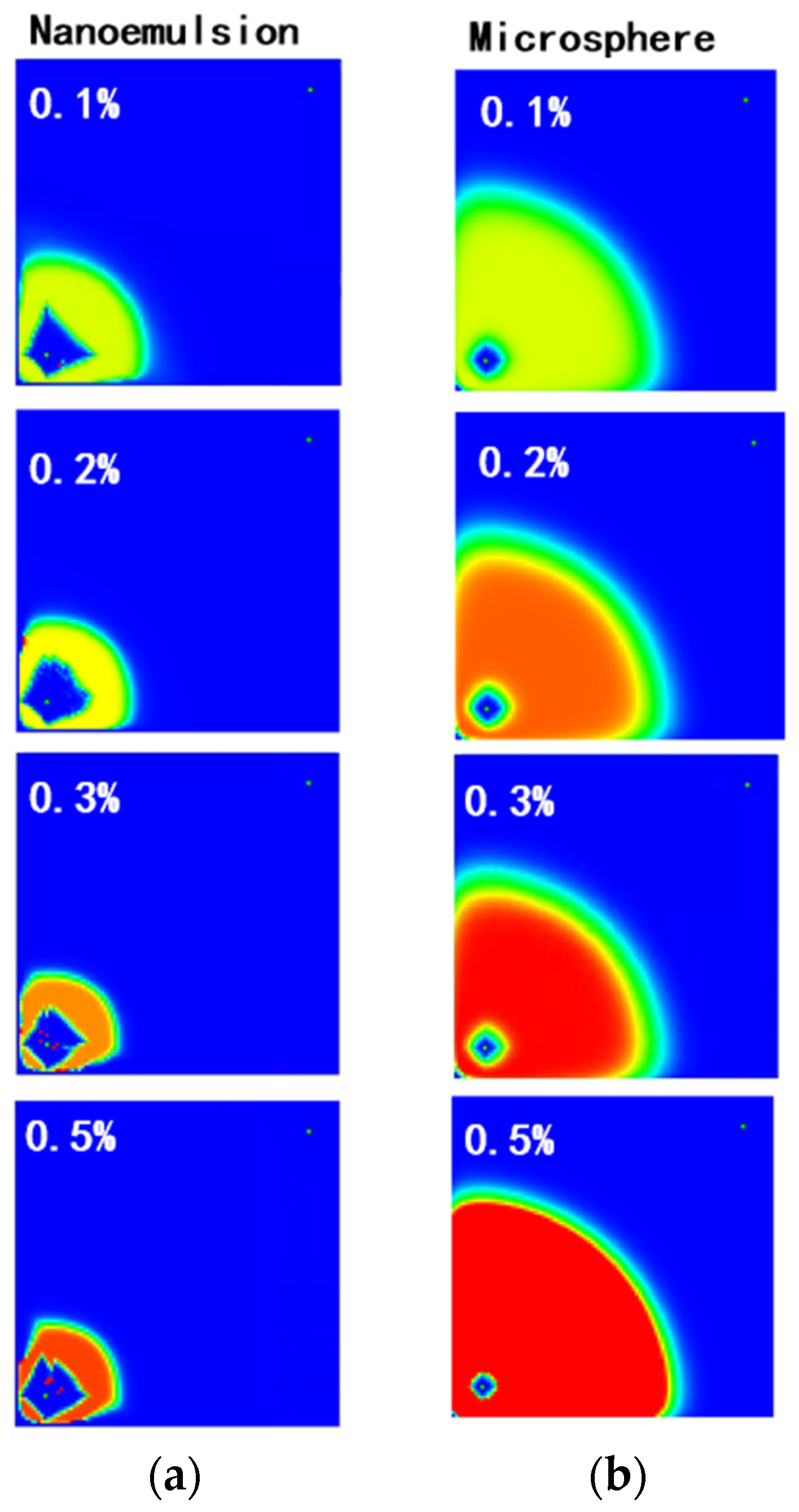
Figure 59.
Component-concentration distribution for different chemical concentrations. (a) nanoemulsion; (b) microspheres. (The colormap represents the concentration of microspheres or Nano emulsion, with red indicating higher concentration.)
Figure 59.
Component-concentration distribution for different chemical concentrations. (a) nanoemulsion; (b) microspheres. (The colormap represents the concentration of microspheres or Nano emulsion, with red indicating higher concentration.)
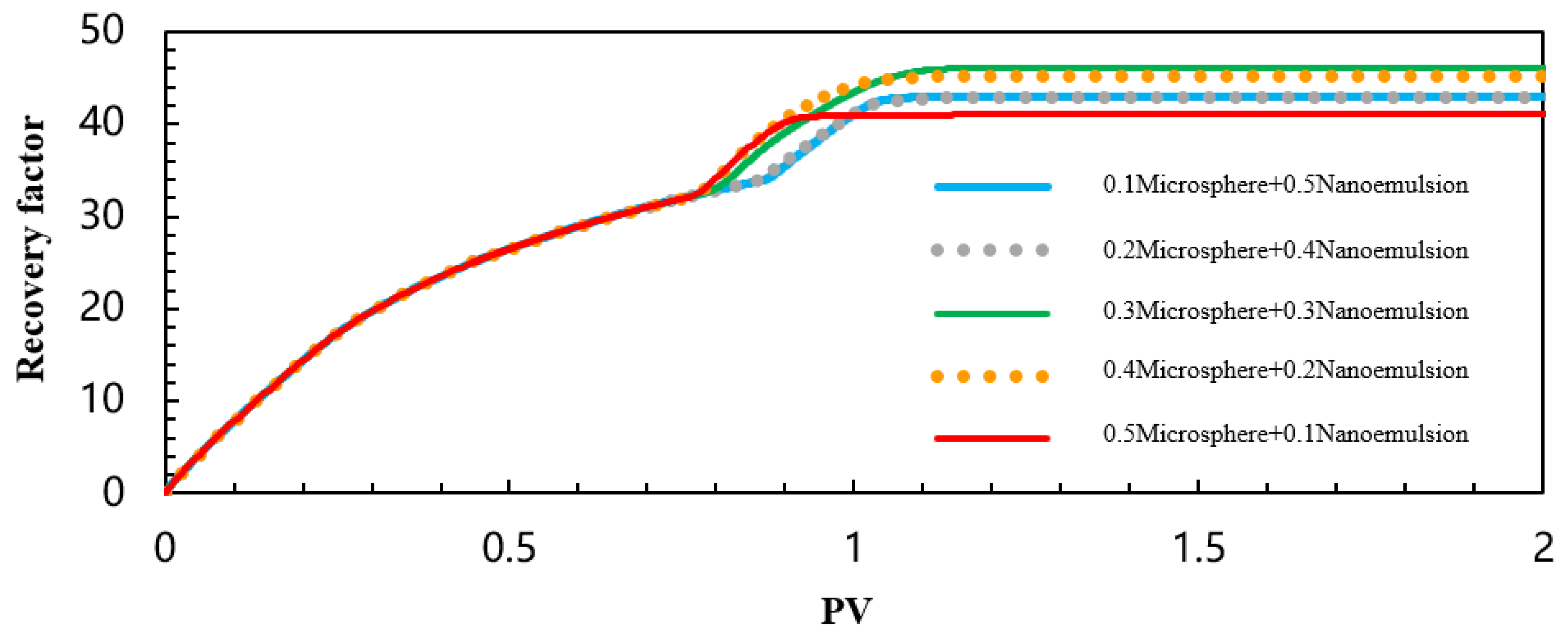
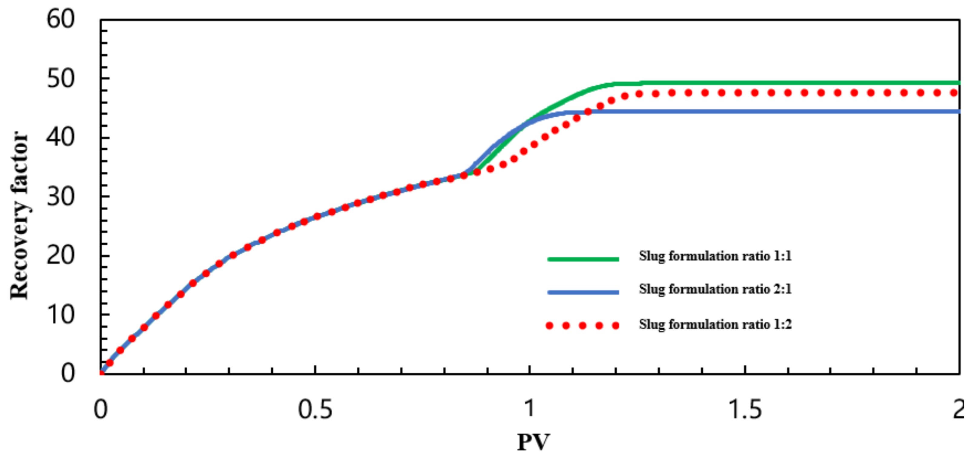
Figure 60.
Oil-recovery curves for dual-slug cases with different slug ratios.
Figure 60.
Oil-recovery curves for dual-slug cases with different slug ratios.
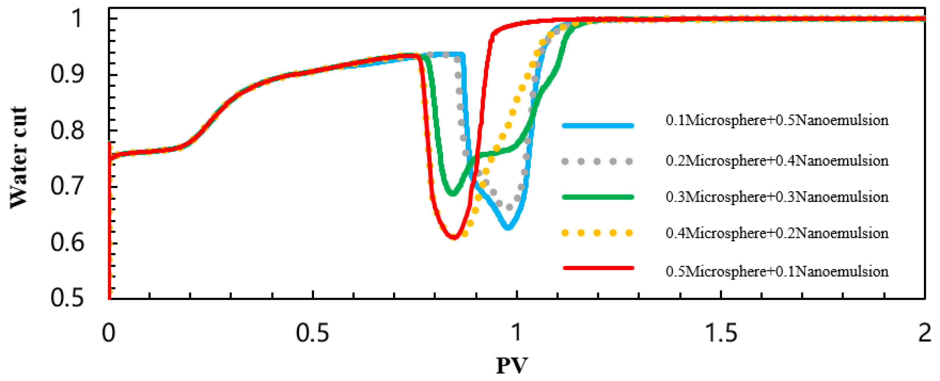
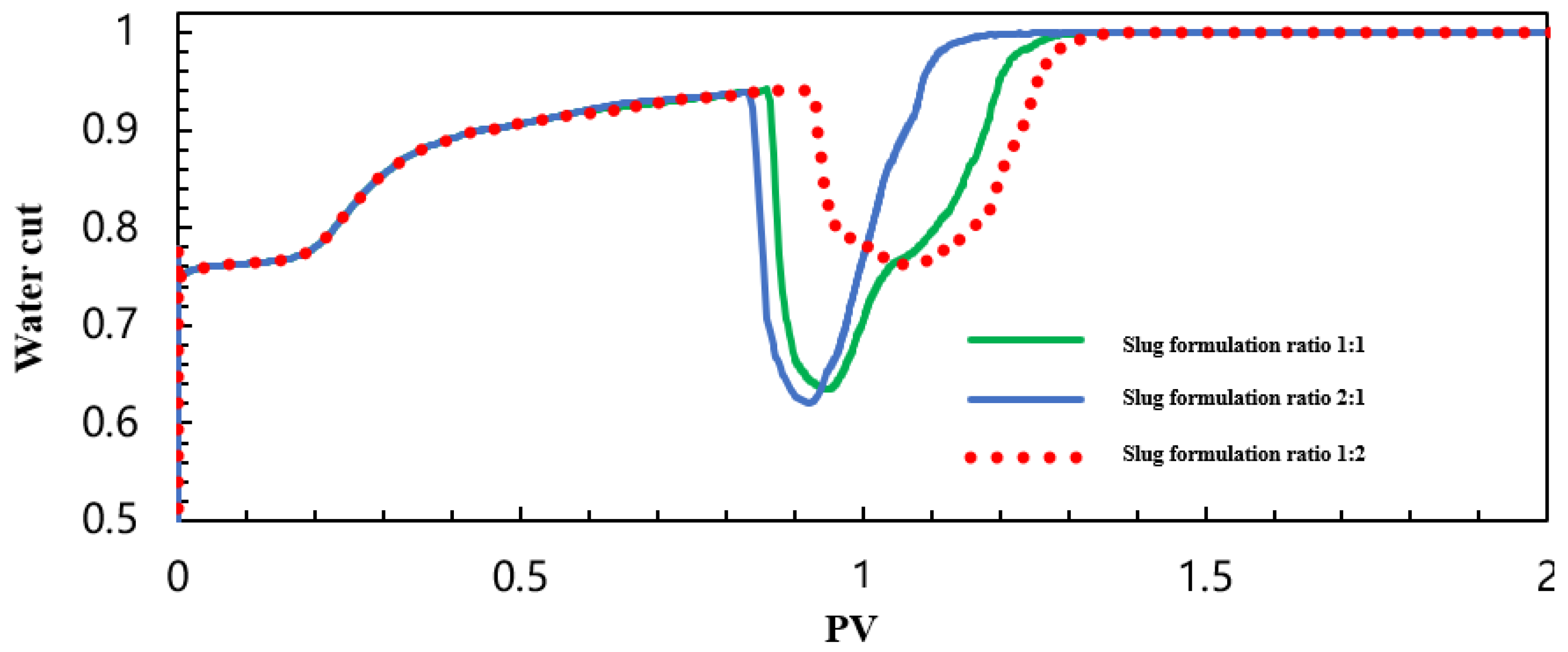
Figure 61.
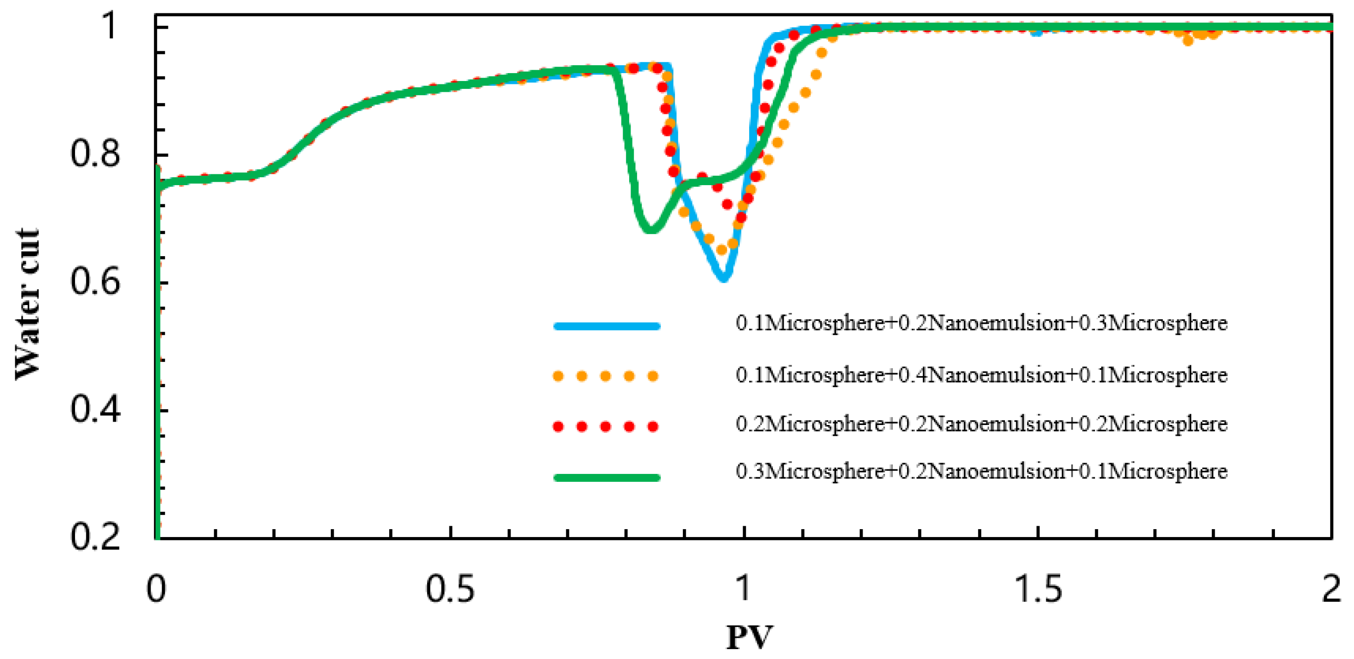
Water-cut curves for dual-slug cases with different slug ratios.
Figure 61.
Water-cut curves for dual-slug cases with different slug ratios.
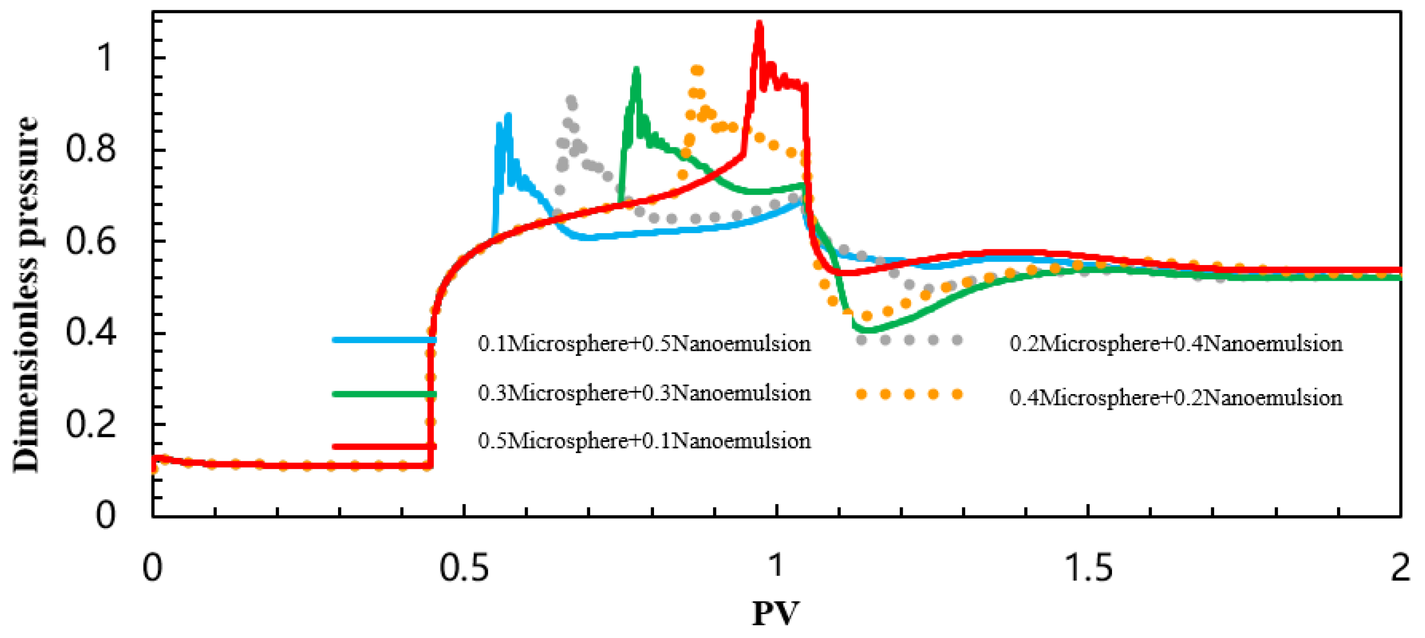
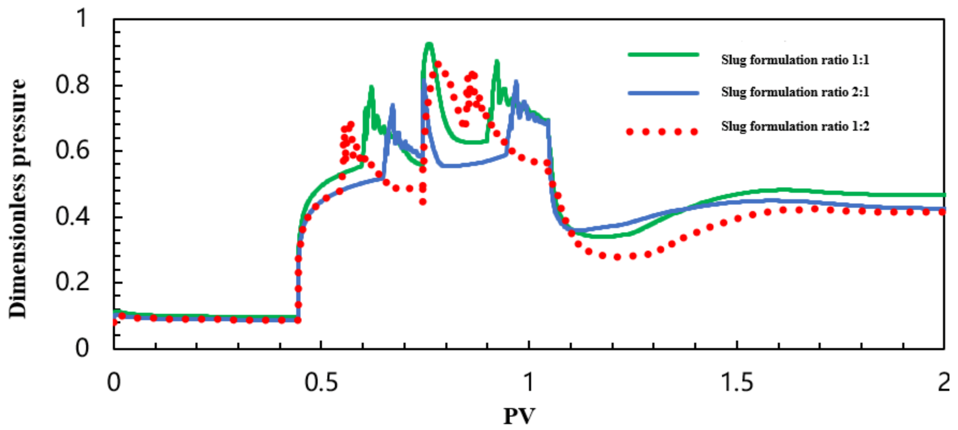
Figure 62.
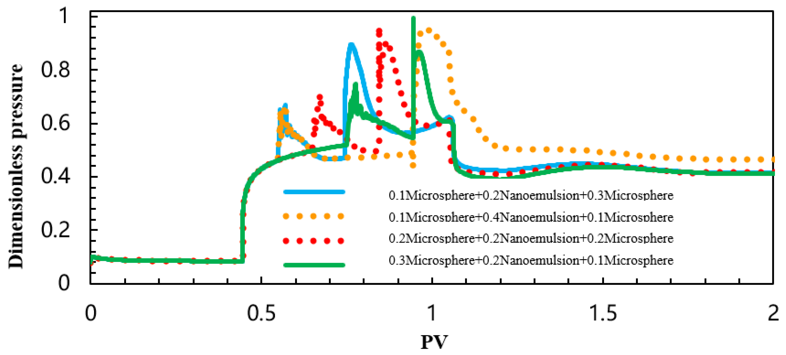
Dimensionless-pressure curves for dual-slug cases with different slug ratios.
Figure 62.
Dimensionless-pressure curves for dual-slug cases with different slug ratios.
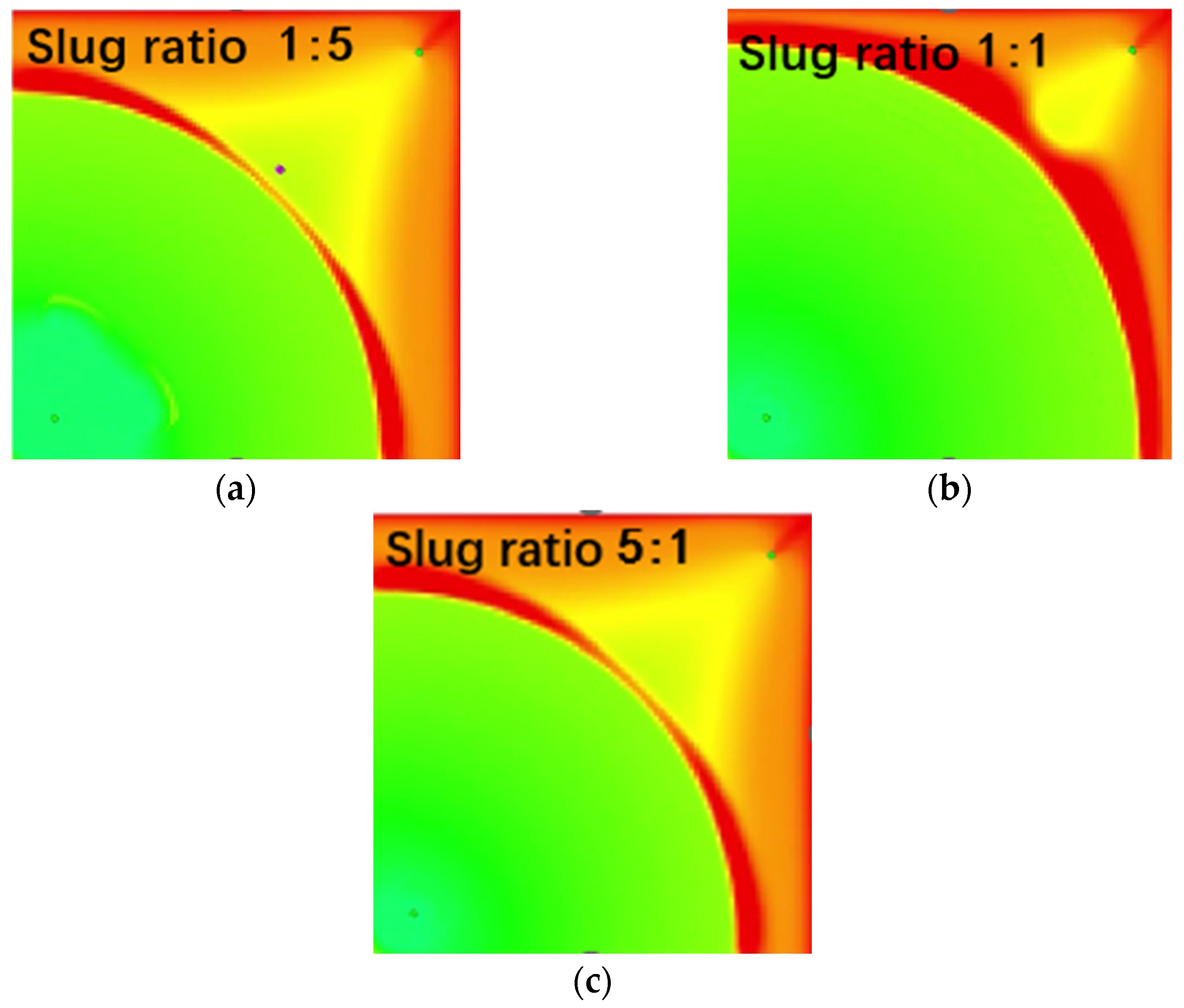
Figure 63.
Oil-saturation distributions for different slug ratios. (a) Slug ratio 1:5; (b) Slug ratio 1:1; (c) Slug ratio 5:1 (the colormap represents oil saturation, with red indicating higher values).
Figure 63.
Oil-saturation distributions for different slug ratios. (a) Slug ratio 1:5; (b) Slug ratio 1:1; (c) Slug ratio 5:1 (the colormap represents oil saturation, with red indicating higher values).
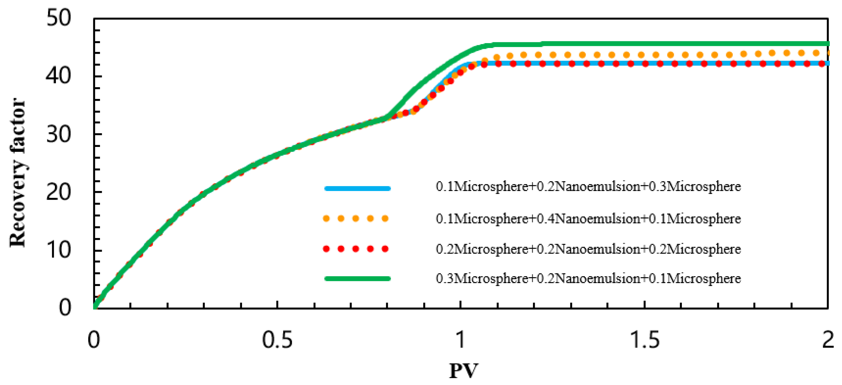
Figure 64.
Oil-recovery curves for three-slug cases with different slug ratios.
Figure 64.
Oil-recovery curves for three-slug cases with different slug ratios.
Figure 65.
Water-cut curves for three-slug cases with different slug ratios.
Figure 65.
Water-cut curves for three-slug cases with different slug ratios.
Figure 66.
Dimensionless-pressure curves for three-slug cases with different slug ratios.
Figure 66.
Dimensionless-pressure curves for three-slug cases with different slug ratios.
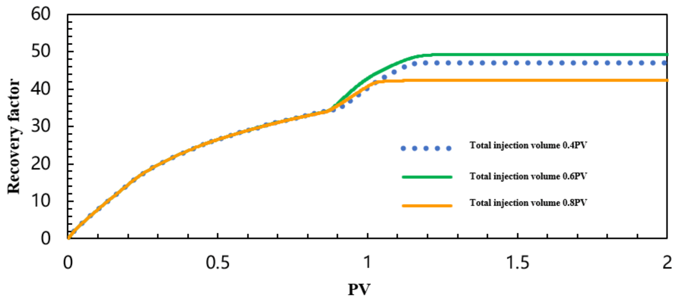
Figure 67.
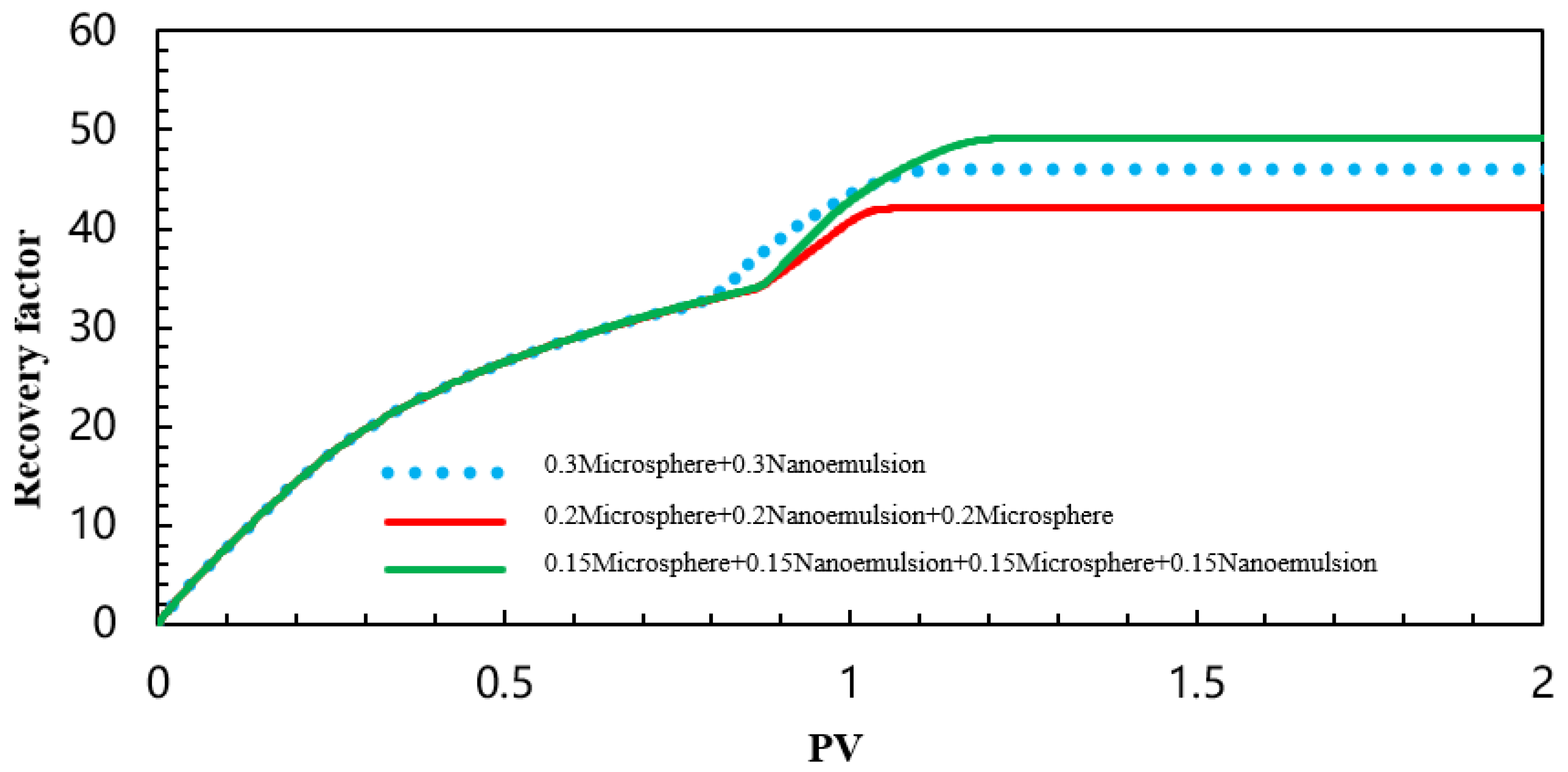
Oil-recovery curves for different slug counts.
Figure 67.
Oil-recovery curves for different slug counts.
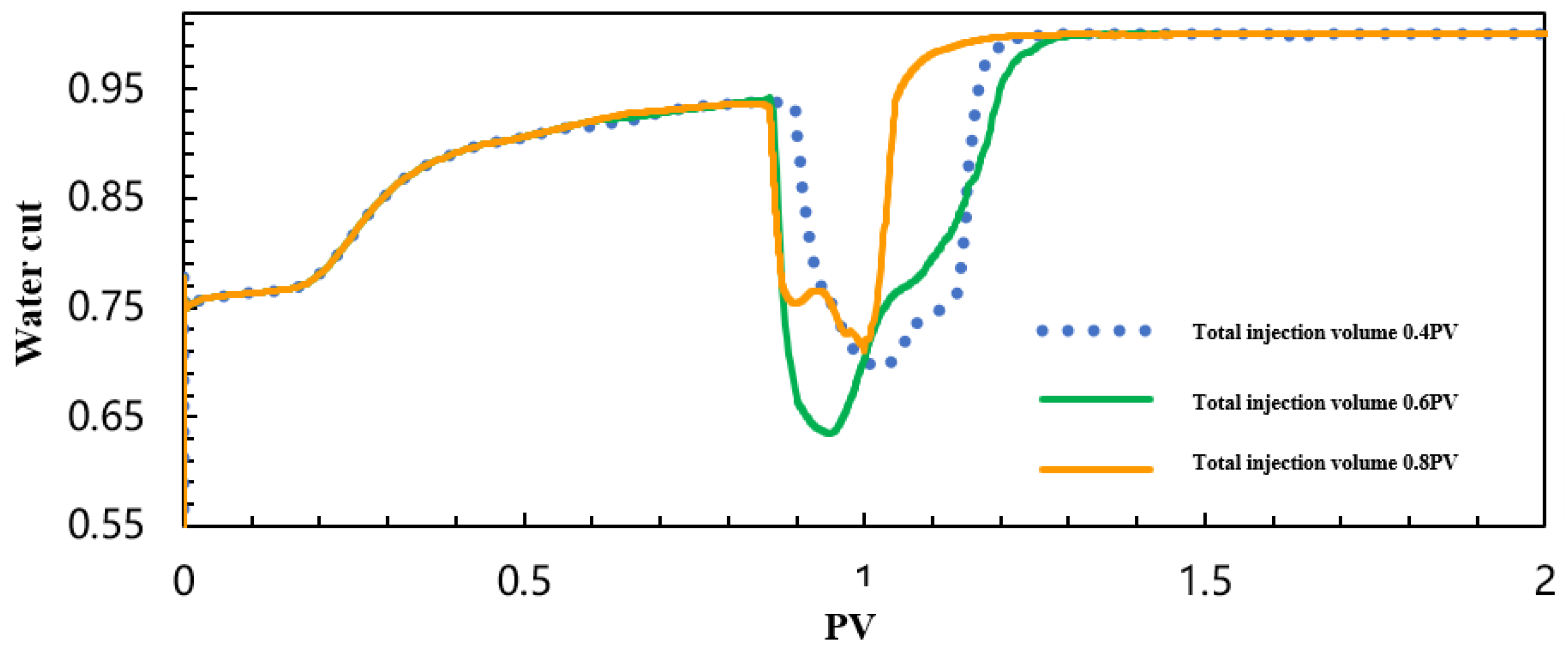
Figure 68.
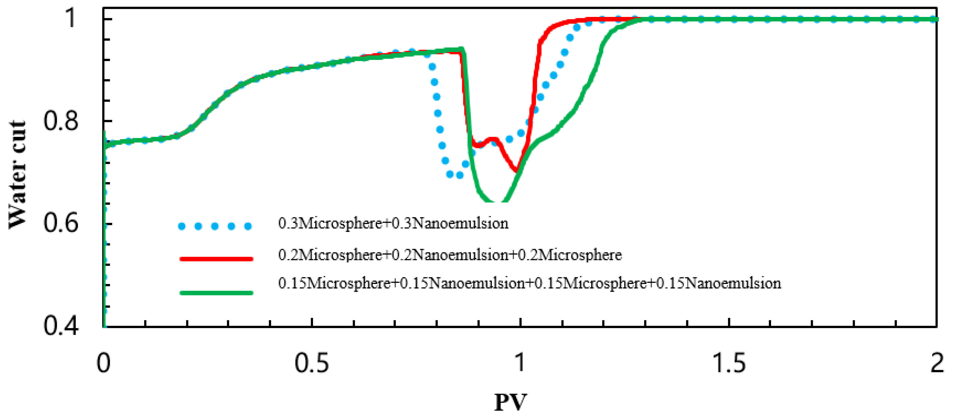
Water-cut curves for different slug counts.
Figure 68.
Water-cut curves for different slug counts.
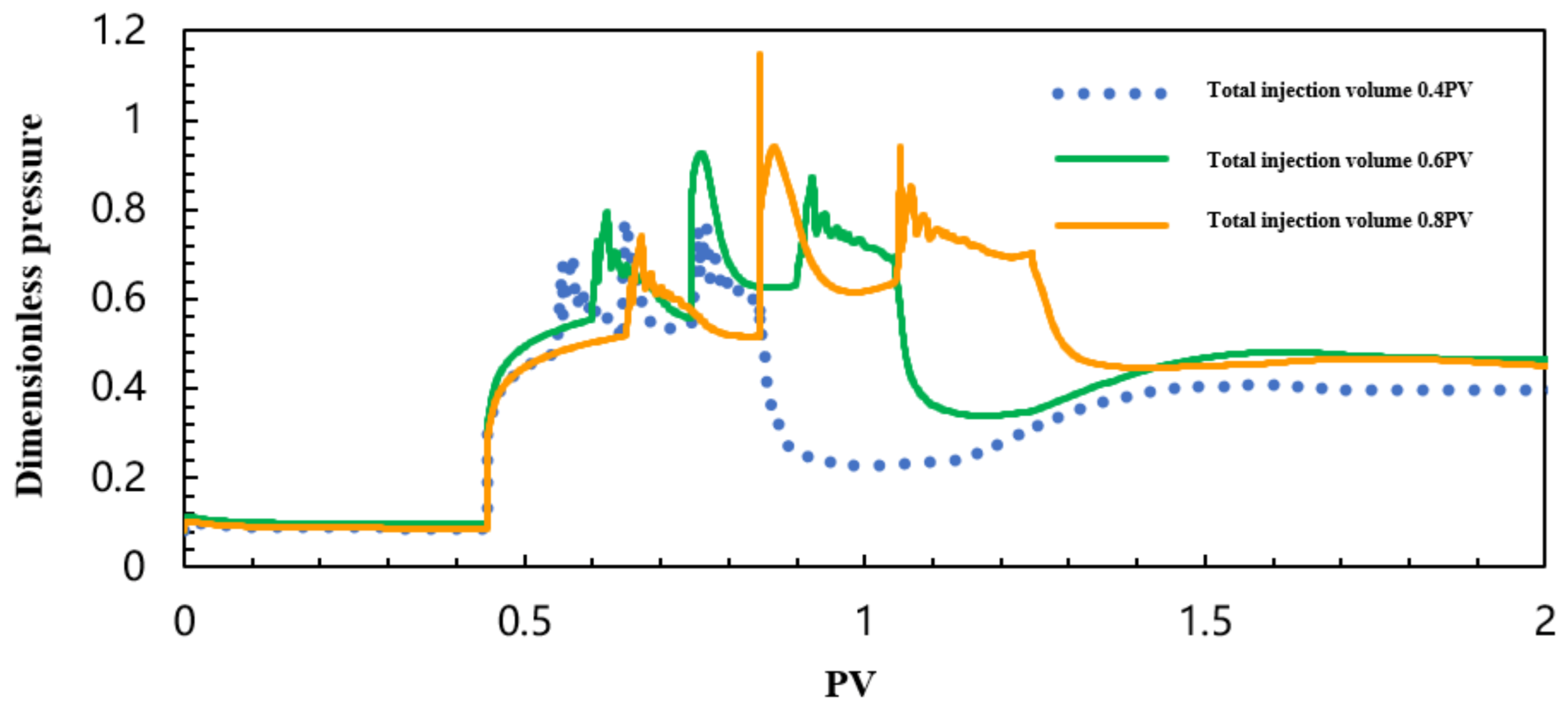
Figure 69.
Dimensionless-pressure curves for different slug counts.
Figure 69.
Dimensionless-pressure curves for different slug counts.
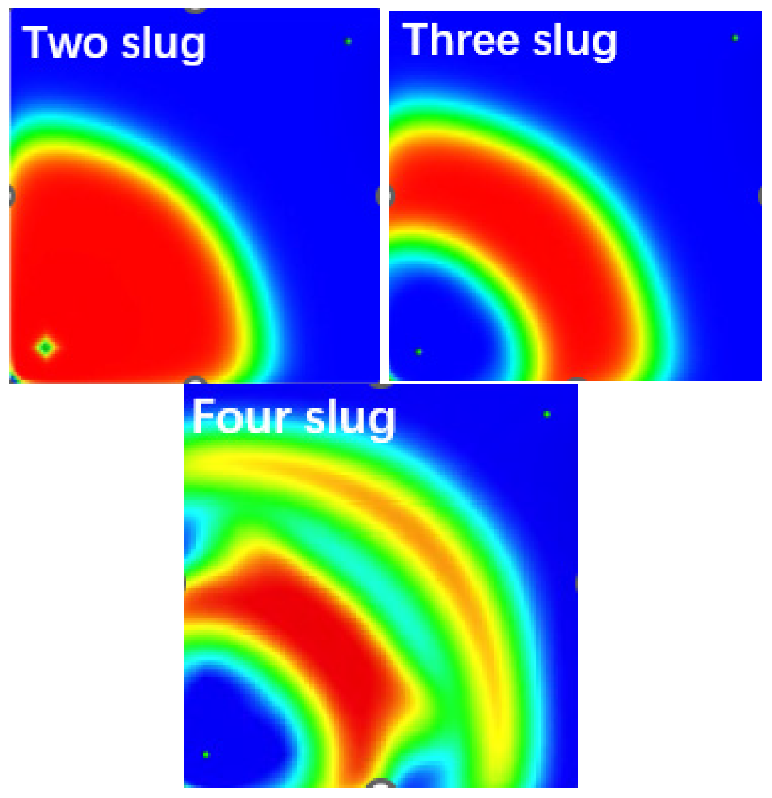
Figure 70.
Non-linear viscosity distributions for different slug counts (the colormap represents viscosity, with red indicating higher values).
Figure 70.
Non-linear viscosity distributions for different slug counts (the colormap represents viscosity, with red indicating higher values).
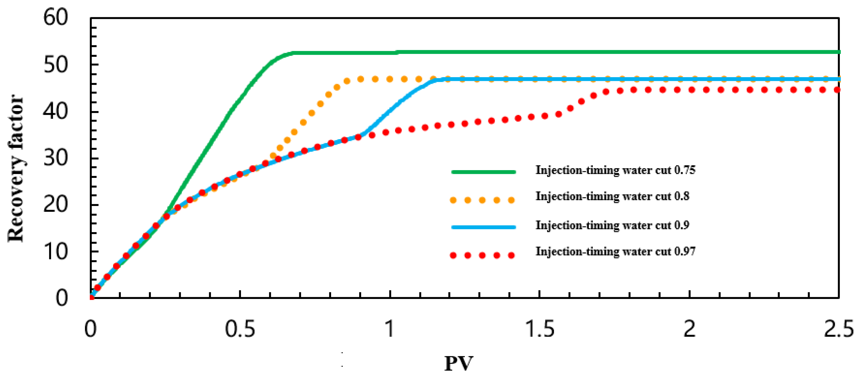
Figure 71.
Oil-recovery curves for different chemical injection timings.
Figure 71.
Oil-recovery curves for different chemical injection timings.
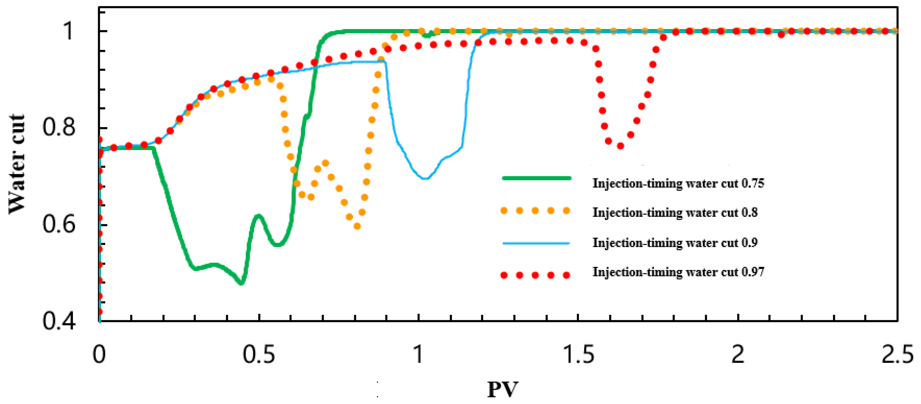
Figure 72.
Water-cut curves for different chemical injection timings.
Figure 72.
Water-cut curves for different chemical injection timings.
Figure 73.
Dimensionless-pressure curves for different chemical injection timings.
Figure 73.
Dimensionless-pressure curves for different chemical injection timings.
Figure 74.
Oil-recovery curves for different slug sizes.
Figure 74.
Oil-recovery curves for different slug sizes.
Figure 75.
Water-cut curves for different slug sizes.
Figure 75.
Water-cut curves for different slug sizes.
Figure 76.
Dimensionless-pressure curves for different slug sizes.
Figure 76.
Dimensionless-pressure curves for different slug sizes.
Figure 77.
Oil-recovery curves for different slug ratios.
Figure 77.
Oil-recovery curves for different slug ratios.
Figure 78.
Water-cut curves for different slug ratios.
Figure 78.
Water-cut curves for different slug ratios.
Figure 79.
Dimensionless-pressure curves for different slug ratios.
Figure 79.
Dimensionless-pressure curves for different slug ratios.
Figure 80.
Representative Well Group 1.
Figure 80.
Representative Well Group 1.
Figure 81.
Representative Well Group 2.
Figure 81.
Representative Well Group 2.
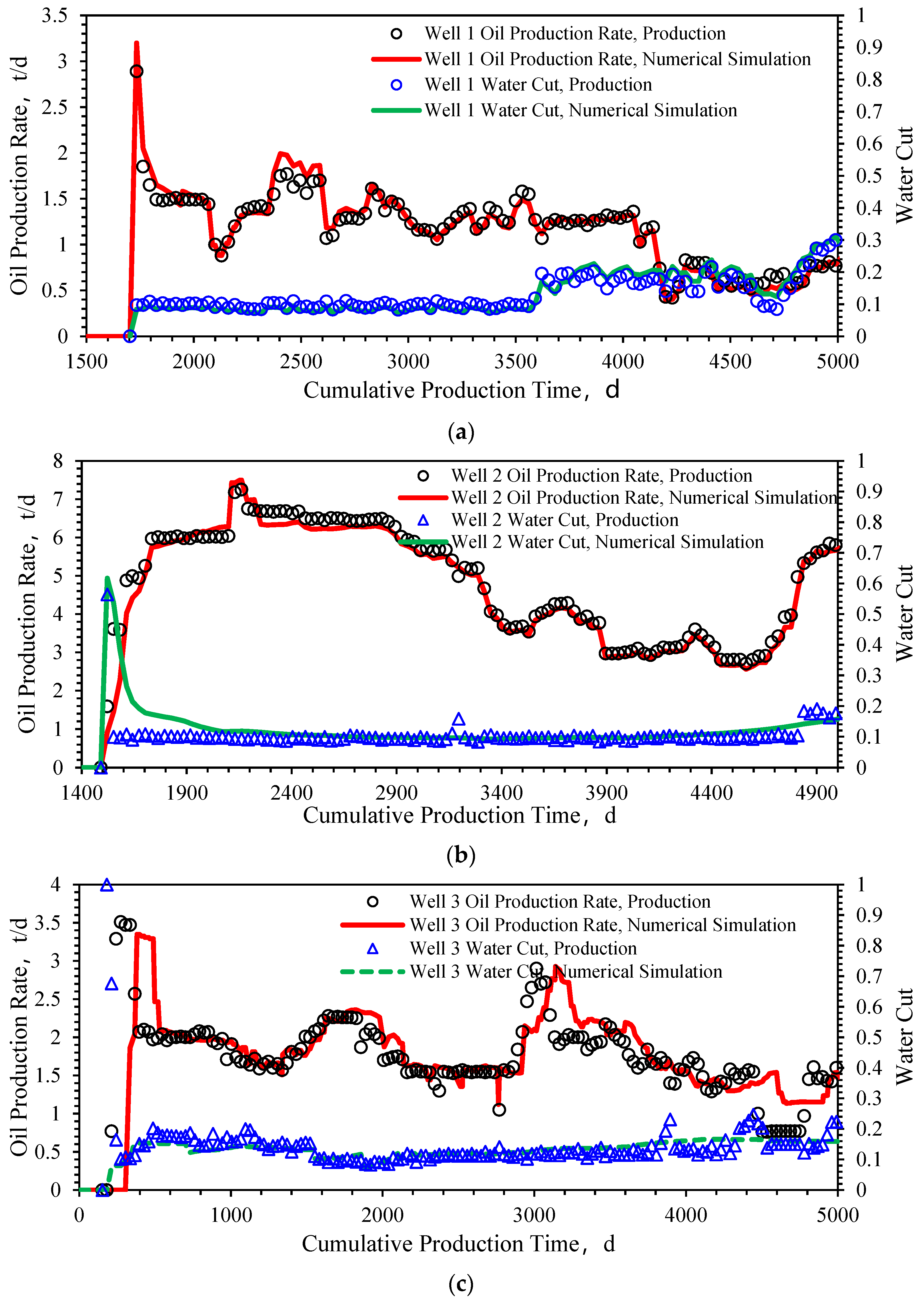
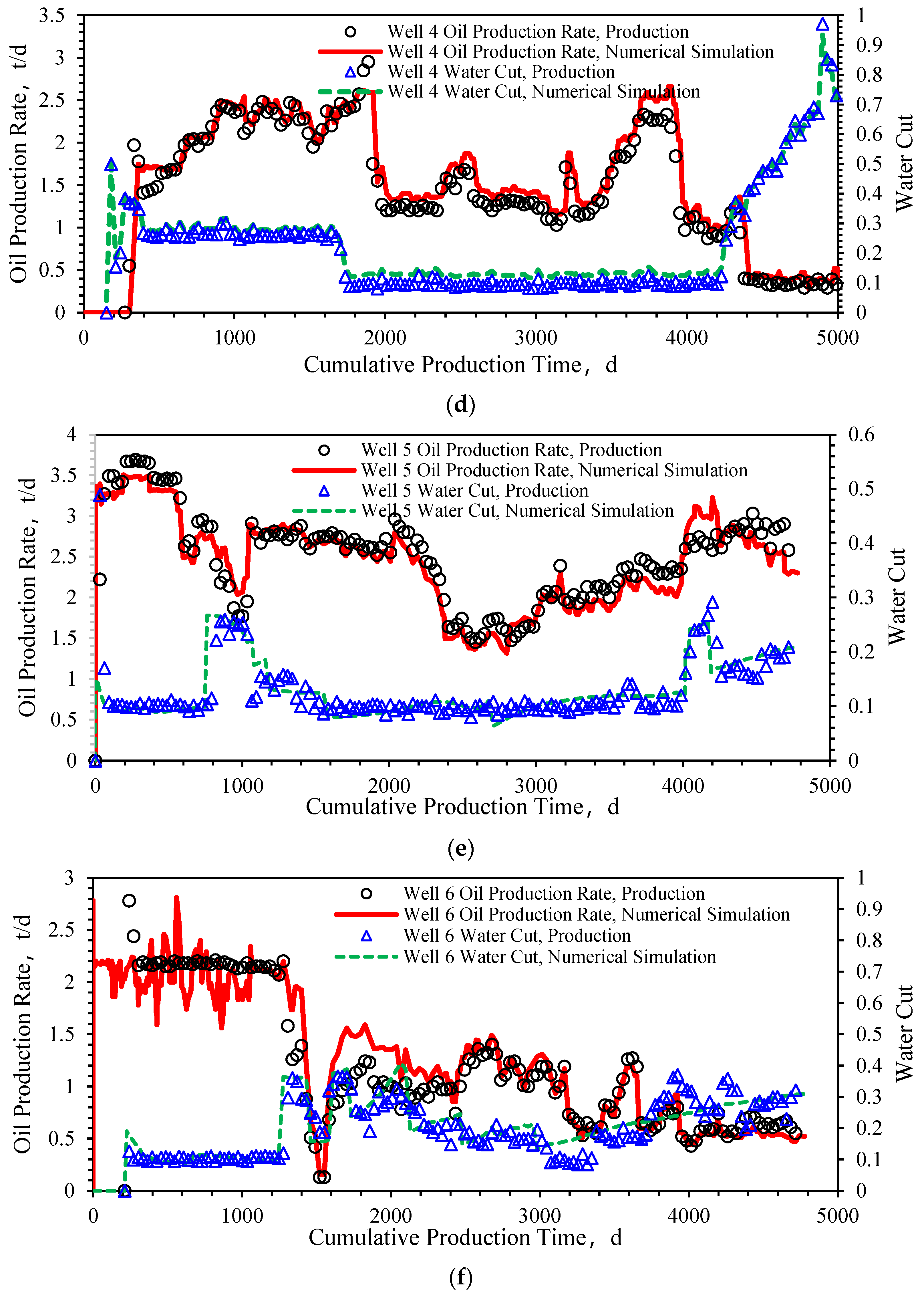
Figure 82.
History matching data for representative well groups, (a) Historical matching data of Well 1 (b) Historical matching data of Well 2 (c) Historical matching data of Well 3 (d) Historical matching data of Well 4 (e) Historical matching data of Well 5 (f) Historical matching data of Well 6.
Figure 82.
History matching data for representative well groups, (a) Historical matching data of Well 1 (b) Historical matching data of Well 2 (c) Historical matching data of Well 3 (d) Historical matching data of Well 4 (e) Historical matching data of Well 5 (f) Historical matching data of Well 6.
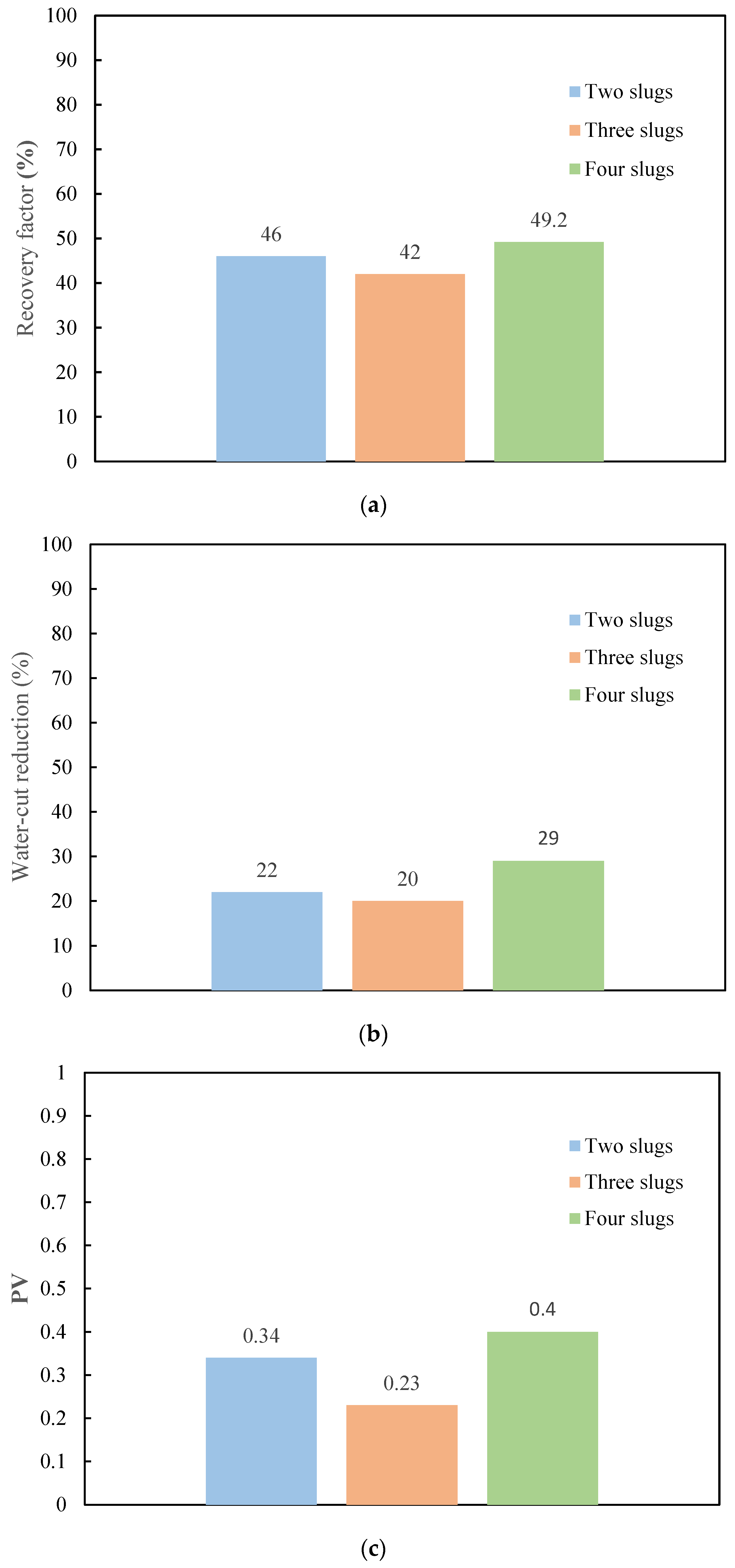
Figure 83.
Parameters diagram of different experimental schemes: (a) represents recovery factor, (b) represents water-cut reduction extent, (c) the water-cut reduction duration in PV injection.
Figure 83.
Parameters diagram of different experimental schemes: (a) represents recovery factor, (b) represents water-cut reduction extent, (c) the water-cut reduction duration in PV injection.
Table 1.
Reservoir conditions.
Table 1.
Reservoir conditions.
| Formation | Temperature
(°C) | Pressure
(MPa) | Permeability
(mD) | Porosity
(%) | Oil Saturation
(%) |
|---|
| Layer C1 | 56 | 15.20 | 5.5 | 12.8 | 53 |
| Layer C2 | 70 | 17.69 | 1.09 | 10.69 | 71 |
Table 2.
Formation water properties.
Table 2.
Formation water properties.
| Formation | Cation (mg·L−1) | Anion (mg·L−1) | pH | TDS |
|---|
| Na+ + K+ | Ca2+ | Mg2+ | Cl− | SO42− | HCO3− | (mg·L−1) |
|---|
| Layer C1 | 26,442 | 4712 | 847 | 48,720 | 723 | 214 | 6 | 81,658 |
| Layer C2 | 10,573.64 | 3997.84 | 375 | 21,634.2 | 152 | 160.93 | 6 | 36,794 |
Table 3.
Core-flood parameters.
Table 3.
Core-flood parameters.
| No. | K
(μm−2 (L-M)) | Porosity
(%) | Length
(cm) | C-S Area
(cm2) | Concentration
(%) | Injection Rate
(mL·min−1) |
|---|
| 1 | 45.7 | 21.3 | 10 | 4.91 | 0.2 | 0.3 |
| 2 | 12.8 | 15.45 |
| 3 | 3.6 | 10.3 |
Table 4.
Key variables at different scales.
Table 4.
Key variables at different scales.
| Experimental Scale | Injection Fluid | Influencing Factors | Key Variable Design |
|---|
| Core Scale L: 6.8~7.7 cm | Microsphere 2.0, Nanoemulsion single-fluid injection | Baseline rock/fluid properties (mD) | 48.70, 15.85, 1.61 |
| D: 2.5 cm | Injection rate (ml/min) | 0.1, 0.2, 0.4 |
| | Injection timing (WC) | 0.5, 0.7, 0.9 |
| | Injection volume (PV) | 0.1, 0.3, 0.5 |
| | Reservoir heterogeneity (mD) | 15.85 + 48.70; 15.85 + 1.61 |
| | Alternating injection | Slug ratio, slug size PV | 1:2, 1:1, 2:1 |
Table 5.
Resistance factor, residual resistance factor, and plugging efficiency for cores of different permeability (0.2% Microsphere2.0).
Table 5.
Resistance factor, residual resistance factor, and plugging efficiency for cores of different permeability (0.2% Microsphere2.0).
| | Core Permeability
(mD) | Water Flooding Pressure (MPa) | Microsphere Injection Pressure (MPa) | Follow-Up Water Flooding Pressure (MPa) | Plugging Efficiency
(%) | Resistance Factor | Residual Resistance Factor |
|---|
| 1 | 287.9 | 0.13 | 0.4384 | 0.35 | 63 | 3.37 | 2.69 |
| 2 | 553.7 | 0.074 | 0.2283 | 0.17 | 56 | 3.09 | 2.3 |
| 3 | 1204.8 | 0.033 | 0.098 | 0.07 | 53 | 2.97 | 2.12 |
| 4 | 2050.4 | 0.021 | 0.06 | 0.036 | 42 | 2.86 | 1.71 |
Table 6.
Experimental parameters for different permeabilities.
Table 6.
Experimental parameters for different permeabilities.
| Key Variables | Experimental Parameters |
|---|
| Absolute permeability (mD) | 1.61/15.85/48.70 |
| Porosity | 0.135, 0.181, 0.194 |
| Initial oil saturation | 0.53, 0.58, 0.71 |
| Injection flow rate (cm3/min) | 0.2 |
| Injected chemical agent | Microspheres 2.0, 0.2% |
| Chemical injection timing | Water cut to 0.9 |
| Chemical injection volume (PV) | 0.3 |
Table 7.
Experimental parameters for injection rates.
Table 7.
Experimental parameters for injection rates.
| Key Variables | Experimental Parameters |
|---|
| Absolute permeability (mD) | 15.85 (Nanoemulsion) |
| 48.70 (Microspheres) |
| Porosity | 0.181, 0.194 |
| Initial oil saturation | 0.58, 0.71 |
| Fluid injection flow rate (cm3/min) | 0.1/0.2/0.4 |
| Injected chemical agent | 0.2% (Microspheres) |
| 0.3% (Nanoemulsion) |
| Chemical injection timing | Water cut to 0.9 |
| Chemical injection volume (PV) | 0.3 |
Table 8.
Experimental parameters for injection timing.
Table 8.
Experimental parameters for injection timing.
| Key Variables | Experimental Parameters |
|---|
| Absolute permeability (mD) | 15.85 (Nanoemulsion) |
| 48.70 (Microspheres) |
| Porosity | 0.181, 0.194 |
| Initial oil saturation | 0.58, 0.71 |
| Fluid injection flow rate (cm3/min) | 0.2 |
| Injected chemical agent | 0.2% (Microspheres) |
| 0.3% (Nanoemulsion) |
| Chemical injection timing | Water cut 0.5/0.7/0.9 |
| Chemical injection volume (PV) | 0.3 |
Table 9.
Experimental parameters for chemical-slug size.
Table 9.
Experimental parameters for chemical-slug size.
| Key Variables | Experimental Parameters |
|---|
| Absolute permeability (mD) | 15.85 (Nanoemulsion) |
| 48.70 (Microspheres) |
| Porosity | 0.181, 0.194 |
| Initial oil saturation | 0.58, 0.71 |
| Fluid injection flow rate (cm3/min) | 0.2 |
| Injected chemical agent | 0.2% (Microspheres) |
| 0.3% (Nanoemulsion) |
| Chemical injection timing | Water cut to 0.9 |
| Chemical injection volume (PV) | 0.1/0.3/0.5 |
Table 10.
Parameters for heterogeneity tests.
Table 10.
Parameters for heterogeneity tests.
| Key Variables | Experimental Parameters |
|---|
| Absolute permeability (mD) | 15.85 + 48.70 |
| 15.85 + 1.61 |
| Porosity | 0.181, 0.194 |
| 0.181 + 0.135 |
| Initial oil saturation | 0.58, 0.71 |
| Fluid injection flow rate (cm3/min) | 0.2 |
| Injected chemical agent | 0.2% (Microspheres) |
| 0.3% (Nanoemulsion) |
| Chemical injection timing | Water cut to 0.9 |
| Chemical injection volume (PV) | 0.3 |
Table 11.
Input parameters for history matching.
Table 11.
Input parameters for history matching.
| Key Variables | Experimental Parameters |
|---|
| Absolute permeability (mD) | 15.85 (Nanoemulsion) |
| 48.70 (Microspheres) |
| Porosity | 0.181, 0.194 |
| Initial oil saturation | 0.58, 0.71 |
| Fluid injection flow rate (cm3/min) | 0.2 |
| Injected chemical agent | 0.2% (Microspheres) |
| 0.3% (Nanoemulsion) |
| Chemical injection timing | Water cut to 0.9 |
| Chemical injection volume (PV) | 0.3 |
Table 12.
Kinetic and flow parameters of the microsphere system.
Table 12.
Kinetic and flow parameters of the microsphere system.
| Types | Parameters | Microsphere 2.0 |
|---|
| Reaction Kinetics Parameters | Slow-Expansion Coefficient FREQFAC1 | 3.4 × 10⁻⁴ |
| Static Decay Coefficient FREQFAC2 | 1.61 × 10⁻⁶ |
| Reaction Stoichiometric Coefficient Si | 443.951 |
| Flow Parameters | Wetting Phase Interpolation Parameter DTRAPW | −3.58 |
| Non-Wetting Phase Interpolation Parameter DTRAPN | −2.95 |
| Maximum Adsorption Capacity ADMAXT (gmole/m3) | 4.98 × 10⁻⁷ |
| Residual Adsorption Capacity ADRT (gmole/m3) | 1.25 × 10⁻⁸ |
| Residual Resistance Factor RRFT | 4 |
Table 13.
Kinetic and flow parameters of the nanoemulsion system.
Table 13.
Kinetic and flow parameters of the nanoemulsion system.
| Types | Parameters | Nanoemulsion |
|---|
| Reaction Kinetics Parameters | Coalescence Reaction Frequency Coefficient FREQFAC1 | 1.4 × 10⁻⁷ |
| Solubilization Reaction Frequency Coefficient FREQFAC2 | 2.15 × 10⁻⁴ |
| Reaction Stoichiometric Coefficient Si | 22.15 |
| Flow Parameters | Wetting Phase Interpolation Parameter DTRAPW | −5.5 |
| Non-Wetting Phase Interpolation Parameter DTRAPN | −5 |
| Aqueous Phase Permeability Endpoint Reduction Factor KRWIRO | 0.35 |
| Oil Phase Permeability Endpoint Reduction Factor KROCW | 0.05 |
| Maximum Adsorption Capacity ADMAXT (gmole/m3) | 5.36 × 10⁻⁶ |
Table 14.
Reservoir model properties.
Table 14.
Reservoir model properties.
| Properties | Value |
|---|
| Reservoir Pressure (MPa) | 15.2 |
| Reservoir Temperature (°C) | 70.8 |
| Porosity | 0.1 |
| Horizontal Permeability (mD) | 1.5~25 |
| Vertical Permeability (mD) | 0.3~3 |
| Initial Oil Saturation (%) | 65 |
| Effective Thickness (m) | 10 |
| Injector-Producer Spacing (m) | 282 |
| Perforated Interval | 5 |
Table 15.
Injection-production design parameters.
Table 15.
Injection-production design parameters.
| Parameters | Value |
|---|
| Liquid Injection Rate (m3/d) | 10, 20, 30, 40, 50, 60 |
| Injection Timing (WC) | 0.75, 0.85, 0.9, 0.97 |
| Injection Volume (PV) | 0.1, 0.2, 0.3, 0.5 |
| Number of Slugs | 1~4 |
| Concentration (%) | Microsphere: 0.1, 0.2, 0.5, 1 |
| Nanoemulsion: 0.2, 0.3, 0.5 |
| Slug Ratio | 1:1, 2:1, 5:1, 1:2, 1:5, 1:1:1, 3:2:1, 1:2:3, 1:4:1 |
| (Microsphere/Nanoemulsion) |
Table 16.
Injection-rate design parameters.
Table 16.
Injection-rate design parameters.
| Parameters | Value |
|---|
| Liquid Injection Rate (m3/d) | 10, 20, 30, 40, 50, 60 |
| Injection Timing (WC) | 0.9 |
| Injection Volume (PV) | 0.3 |
| Concentration (%) | Microsphere: 0.2 |
| Nanoemulsion: 0.3 |
Table 17.
Injection-timing design parameters.
Table 17.
Injection-timing design parameters.
| Parameters | Value |
|---|
| Liquid Injection Rate (m3/d) | 30 |
| Injection Timing (WC) | 0.75, 0.85, 0.9 |
| Injection Volume (PV) | 0.3 |
| Concentration (%) | Microsphere: 0.2 |
| Nanoemulsion: 0.3 |
Table 18.
Slug-size design parameters.
Table 18.
Slug-size design parameters.
| Parameters | Value |
|---|
| Liquid Injection Rate (m3/d) | 30 |
| Injection Timing (WC) | 0.9 |
| Injection Volume (PV) | 0.1, 0.2, 0.3, 0.5 |
| Concentration (%) | Microsphere: 0.2 |
| Nanoemulsion: 0.3 |
Table 19.
Chemical concentration design parameters.
Table 19.
Chemical concentration design parameters.
| Parameters | Value |
|---|
| Liquid Injection Rate (m3/d) | 30 |
| Injection Timing (WC) | 0.9 |
| Injection Volume (PV) | 0.3 |
| Concentration (%) | Microsphere: 0.1, 0.2, 0.3, 0.5 |
| Nanoemulsion: 0.1, 0.2, 0.3, 0.5 |
Table 20.
Dual-slug injection-production parameters.
Table 20.
Dual-slug injection-production parameters.
| Parameters | Value |
|---|
| Liquid Injection Rate (m3/d) | 30 |
| Injection Timing (WC) | 0.9 |
| Injection Volume (PV) | 0.6 |
| Number of Slugs | 2 |
| Concentration (%) | Microsphere: 0.2 |
| Nanoemulsion: 0.3 |
| Slug Ratio (Microsphere/Nanoemulsion) | 1:1, 2:1, 5:1, 1:2, 1:5 |
Table 21.
Three-slug injection-production parameters.
Table 21.
Three-slug injection-production parameters.
| Parameters | Value |
|---|
| Liquid Injection Rate (m3/d) | 30 |
| Injection Timing (WC) | 0.9 |
| Injection Volume (PV) | 0.6 |
| Number of Slugs | 3 |
| Concentration (%) | Microsphere: 0.2 |
| Nanoemulsion: 0.3 |
| Slug Ratio (Microsphere/Nanoemulsion/Microsphere) | 1:1:1, 3:2:1, 1:2:3, 1:4:1 |
Table 22.
Injection-production parameters for different slug counts.
Table 22.
Injection-production parameters for different slug counts.
| Parameters | Value |
|---|
| Liquid Injection Rate (m3/d) | 30 |
| Injection Timing (WC) | 0.9 |
| Injection Volume (PV) | 0.6 |
| Number of Slugs | 2, 3, 4 |
| Concentration (%) | Microsphere: 0.2 |
| Nanoemulsion: 0.3 |
| Slug Ratio (Microsphere/Nanoemulsion) | 1:01 |
Table 23.
Injection-production parameters for different injection timing.
Table 23.
Injection-production parameters for different injection timing.
| Parameters | Value |
|---|
| Liquid Injection Rate (m3/d) | 30 |
| Injection Timing (WC) | 0.75, 0.8, 0.9, 0.97 |
| Injection Volume (PV) | 0.6 |
| Number of Slugs | 4 |
| Concentration (%) | Microsphere: 0.2 |
| Nanoemulsion: 0.3 |
| Slug Ratio (Microsphere/Nanoemulsion) | 1:01 |
Table 24.
Injection-production parameters for different slug sizes.
Table 24.
Injection-production parameters for different slug sizes.
| Parameters | Value |
|---|
| Liquid Injection Rate (m3/d) | 30 |
| Injection Timing (WC) | 0.9 |
| Injection Volume (PV) | 0.4, 0.6, 0.8 |
| Number of Slugs | 4 |
| Concentration (%) | Microsphere: 0.2 |
| Nanoemulsion: 0.3 |
| Slug Ratio (Microsphere/Nanoemulsion) | 1:01 |
Table 25.
Injection-production parameters for different slug ratios.
Table 25.
Injection-production parameters for different slug ratios.
| Parameters | Value |
|---|
| Liquid Injection Rate (m3/d) | 30 |
| Injection Timing (WC) | 0.9 |
| Injection Volume (PV) | 0.6 |
| Number of Slugs | 4 |
| Concentration (%) | Microsphere: 0.2 |
| Nanoemulsion: 0.3 |
| Slug Ratio (Microsphere/Nanoemulsion) | 1:1, 2:1, 1:2 |




 and
and