Article

Real-Time Prediction of Bottom Hole Pressure via Graph Neural Network

1
College of Petroleum Engineering, China University of Petroleum, Beijing 102249, China
2
CNOOC Research Institute Co., Ltd., Beijing 100010, China
*
Authors to whom correspondence should be addressed.
Processes 2025, 13(12), 4081; https://doi.org/10.3390/pr13124081
Submission received: 15 November 2025 / Revised: 9 December 2025 / Accepted: 16 December 2025 / Published: 18 December 2025
(This article belongs to the Special Issue Modeling, Control, and Optimization of Drilling Techniques)

Abstract

Accurately and efficiently predicting bottomhole pressure (BHP) is of great importance for safe drilling in complex formations. Many researchers have conducted extensive investigations into intelligent BHP prediction techniques. However, the current intelligent models mostly focus on the data-driven relationship between logging parameters and BHP, and less on the influence of the correlation between the logging parameters on the BHP. This paper proposes a real-time prediction framework based on graph neural networks. Our model selects input features based on drilling mechanisms and statistical analyses, and utilizes adaptive learning of the graph based on multivariate time-series parameters to capture the relationship between multivariate logging parameters and BHP. Finally, the model performance is thoroughly analyzed based on field drilling datasets after optimizing model hyperparameters using the Bayesian optimization method. Results indicate that the proposed method performs better in terms of prediction accuracy, captures the inflection points of curve changes better, and is more robust under the new well section. The mean absolute percentage error of the method reaches 1.28% which is reduced by 25% compared with other traditional intelligent models. This study provides a solution for achieving accurate real-time predictions of bottom hole pressure, establishing a solid foundation for the realization of precise pressure control during drilling operations.

1. Introduction

Bottomhole pressure (BHP) is a critical hydraulic indicator that ensures the wellbore pressure remains within the safe operating window during drilling [1]. Any deviation from this window can trigger severe downhole incidents: excessive BHP may induce lost circulation, differential sticking, or wellbore instability due to excessive hydraulic stress on the formation; insufficient BHP can lower the effective barrier against formation pressure, leading to gas influx, well kicks, and even blowouts. However, BHP is jointly influenced by complex factors such as displacement, trajectory, fluid properties, and transient gas intrusion, resulting in strong nonlinear fluctuations. Conventional empirical formulas often fail to address this complexity and thus yield large errors, while numerical approaches depend on predefined assumptions and lack real-time applicability. Although downhole pressure sensors can provide direct measurements, they are costly to deploy, susceptible to data distortion and transmission constraints, and therefore cannot fully meet the requirements of high-frequency, real-time monitoring in field operations. These challenges highlight the necessity for a more accurate and adaptive BHP prediction method capable of capturing dynamic downhole conditions.
In recent years, artificial intelligence has emerged as a powerful tool for addressing multi-parameter and nonlinear complex engineering problems, ushering in a transformative era in drilling technology [2], which has achieved a variety of studies, including drilling quality [3,4], drilling safety [5,6,7], and drilling efficiency [8,9]. Many researchers have increasingly turned to machine learning methods to predict BHP, which has been significantly improved in accuracy and efficiency. Some scholars [7,10,11] have utilized various structures of artificial neural network (ANN) to accurately calculate BHP. Okoro et al. [11] collected downhole pressure data from six wells with drilling measurement devices, establishing two high-precision BHP prediction models based on extreme random tree and feed-forward neural network, respectively. To further enhance the prediction accuracy of the models, several researchers have constructed hybrid network models. Zhang et al. [1] established a hybrid neural network model of Convolutional Neural Network (CNN) and attention-Gate Recurrent Unit (GRU) based on real-time logging data in the field, demonstrating its superiority over a single-network approach in predicting BHP. In addition, scholars have investigated the generalization of the model [12], which combines data expansion and transfer learning methods to ensure accurate predictions in different well sections.
Despite these advancements, BHP remains a complex parameter affected by various factors, exhibiting strong volatility and temporal sequence dependencies. It is difficult to collect data in real time from complex well sections such as high temperature and high pressure, and the large interval between data measurement points and the difficulty of transmission make it difficult to respond to the complex downhole conditions in a timely manner. Furthermore, the existing data-driven models, due to their sensitivity, have not adequately considered the combined effects of the multiple interacting parameters on BHP. Compared to traditional temporal networks, Graph Neural Networks (GNNs) present a promising solution, capable of capturing diverse and complex relationships within features and the temporal contexts in the sequences. Graph-based modeling approaches have demonstrated success in various domains such as transportation, ocean, and drilling [13,14,15]. Therefore, this paper proposes a real-time prediction method for BHP based on an Improved Hybrid Graph Learning Network (IHGLN). The graph learning layer adaptively learns multivariate relationships in different downhole environments to enhance model stability under varying data conditions. The combination of the temporal feature extractor and the graph convolution layer effectively captures high-dimensional features influencing bottomhole pressure variations, resulting in accurate predictions. This study can provide valuable technical support for the efficient and accurate prediction of bottomhole pressure, providing field engineers with guidance for implementing pressure control measures effectively and scientifically.

2. Methodology

In this paper, we propose a graph learning framework to examine the impact on prediction of BHP under the temporal variation in key factors and their interactions. The experimental dataset, the overall model architecture, and the setup of the training process are described in the subsequent sections.

2.1. Datasets

The data used in this study originate from a drilling well in the Tarim Basin, China, with a maximum vertical depth of 4942 m and a measured depth of 6705 m. Based on hydraulic mechanism analysis and literature research [1,12,16], thirteen drilling operations and mud parameters influencing bottomhole pressure are selected as model inputs.
To ensure data quality and improve the robustness of the model, multiple pre-processing operations are applied. First, the 3σ rule is used for outlier removal [17], since extreme deviations may arise from downhole sensor interference or transient drilling disturbances and could misguide the training process if retained. Linear interpolation is then applied to reconstruct missing records while maintaining the continuity of the drilling time series. Considering that downhole measurements are often affected by random noise and operational fluctuations, a sliding window technique is introduced [18,19] to construct subsequences with contextual information, enabling the model to more effectively learn the temporal evolution and dynamic coupling relationships among parameters.
After cleaning, the characteristics of the selected data are presented in Table 1. Data normalization is performed to eliminate the influence of different parameters on the bottomhole pressure. This paper utilizes the maximum-minimum normalization calculation method, mapping the characteristic variables to the (0, 1) range according to the formula:
x ~ = x x min x max x min
where x ~ denotes a feature after normalization, x is an original feature, x m i n represents the minimum value of the feature, x m a x represents the maximum value of the feature.
The processed dataset is divided in the ratio of 8:2, and a total of 64,000 samples are utilized to train the model, and a total of 16,000 samples are reserved for testing the model’s performance.

2.2. Feature Engineering

Influencing factors of BHP involve complex hydraulic, mechanical, and thermodynamic interactions along the wellbore. To ensure the physical interpretability and computational efficiency of the proposed model, feature engineering is performed to refine the input variables before model construction.
(1)
Mechanism-driven initial feature screening
Based on drilling hydraulic principles, thirteen variables closely related to BHP variations are initially selected, including geometric parameters (measured depth, fixed vertical depth), fluid characteristics (drilling fluid density, outlet density, outlet temperature, funnel viscosity, sand content), hydraulic operating parameters (standpipe pressure, inlet/outlet flow rate, back-pressure pump flow rate), and drilling mechanical control (rotary speed), as well as surface system state indicators (total pit volume). These parameters collectively influence static pressure, frictional pressure loss, and transient flow behavior, forming a physically comprehensive input foundation for BHP prediction.
(2)
Correlation-based feature selection
To further reduce redundancy, enhance prediction accuracy, avoid multicollinearity, and improve interpretability and computational performance, Pearson correlation analysis is applied to quantify linear relationships among the variables and between each input variable and the BHP target. Pearson correlation coefficient rxy ranges from −1 to 1, describing the strength and direction of linear correlation:
r x y = C o v ( X , Y ) σ X σ Y
where C o v ( X , Y ) denotes the covariance between X and Y , and σ X and σ Y represent their standard deviations.
A correlation heatmap is constructed based on the computed coefficients. As shown in Figure 1, the sand content remains almost constant in our dataset and therefore provides little informative variability for the model. Consequently, this variable is removed from the input parameters. The final feature subset is determined to balance physical completeness and model efficiency, ensuring a solid data foundation for BHP prediction.

2.3. Improved Hybrid Graph Learning Network

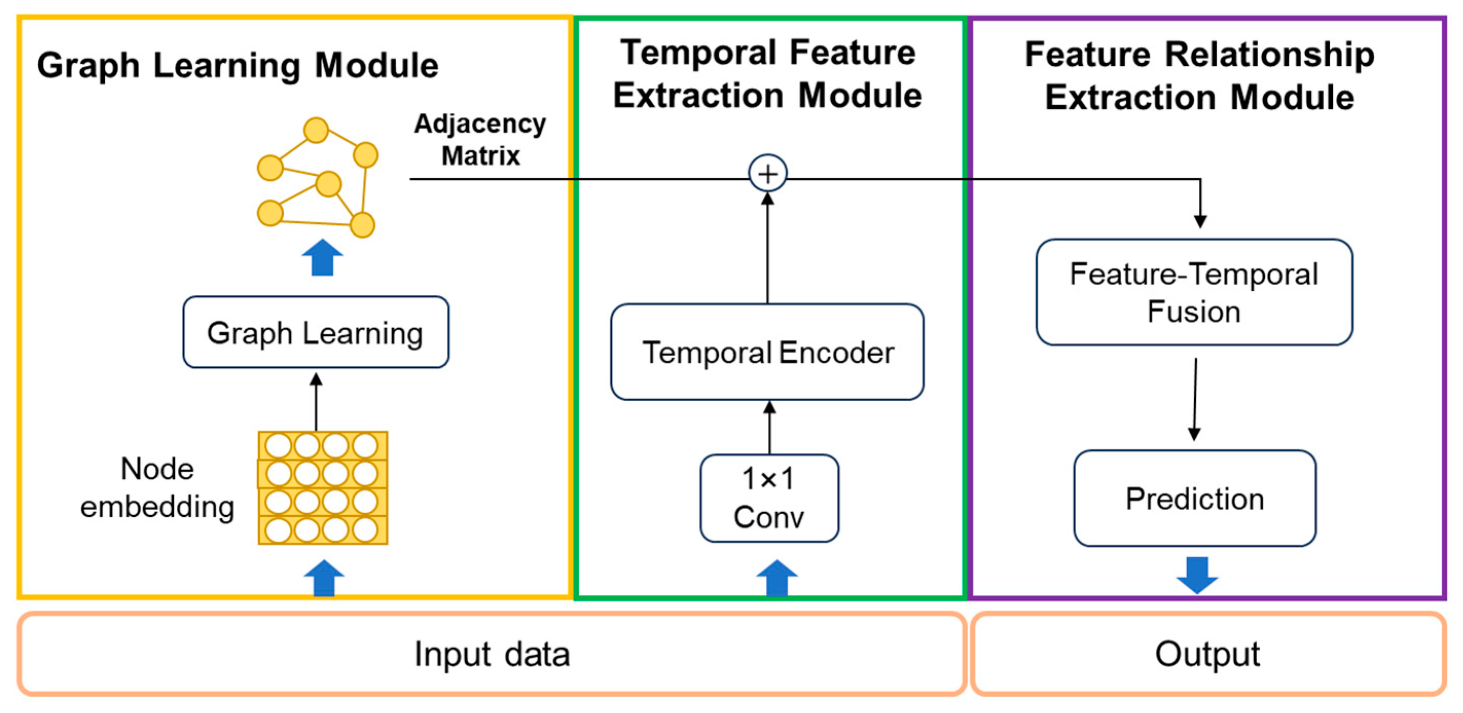
To address the strong temporal fluctuations and dynamically changing parameter correlations inherent in the drilling process, this paper proposes a real-time BHP prediction model based on an Improved Hybrid Graph Learning Network (IHGLN). The main architecture of the model consists of three modules—graph learning layer, temporal feature extraction module, and feature relationship extraction module, as illustrated in Figure 2. The overall workflow is designed to simultaneously capture the temporal evolution of drilling parameters and the non-stationary multivariate interactions that jointly influence BHP changes. Specifically, the graph learning module adaptively constructs a data-driven feature association graph to overcome the limitation of pre-defined static feature relationships, while the temporal feature extraction module focuses on learning high-dimensional dynamic patterns within the time domain. Finally, the feature relationship extraction module fuses structural dependencies and temporal representations to strengthen the model’s capability in identifying pressure fluctuation characteristics and inflection points.
(3)
Graph learning module
The graph learning layer is responsible for describing the dynamic relationships among drilling parameters. Due to frequent lithology variations, hydraulic disturbances, and potential gas invasion, the correlations between parameters vary over time. Therefore, instead of relying on expert-defined prior graphs, the model adaptively constructs an adjacency matrix Aj based on real-time node embeddings, enabling a more realistic representation of parameter interactions. The adjacency matrix guides the downstream extraction of inter-feature influence relationships and improves model robustness under varying data distributions. The initial step involves subjecting the input data to node embedding, followed by relational mapping using a linear layer. By employing Tanh and Relu activation functions, the result is the generation of the adjacency matrix, denoted as Aj, which serves as a representation of a feature association graph (variable × variable). This process is outlined as follows:
E 1 = t a n h ( W 1 X t ) ,   E 2 = t a n h ( W 2 X t )
A j = R e l u ( t a n h ( E 1 E 2 T ) )
where W1 and W2 are the weight matrices and E1 and E2 denote the original node embedding and the target node embedding, which are both trainable parameters.
Notably, this graph learning module can automatically mine the implicit influence relationships among drilling parameters, rather than relying on manually designed correlations or prior physical assumptions. This not only provides a more flexible and accurate representation of the drilling dynamics but also offers better interpretability, since the learned feature association graph explicitly reveals how different parameters affect BHP under varying operating conditions.
(4)
Temporal feature extraction module
In the IHGLN structure, the temporal feature extraction module utilizes the TCN network architecture [20] to receive input parameter information from a 1 × 1 Conv layer. The network is designed for sequence modeling tasks, which contains five components. At its core, TCN utilizes one-dimensional convolutions to discern temporal dependencies within input sequences. What sets TCN apart is its incorporation of dilated convolutions, which enable the network to capture both short-term and long-term temporal relationships efficiently. The dilation factor introduces gaps between filter elements, expanding the receptive field without a substantial increase in parameters. To address training challenges, TCN often integrates residual connections between convolutional layers, facilitating the flow of gradients during optimization. Moreover, TCN employs causal convolutions to respect the temporal order of input sequences, ensuring predictions rely solely on past and present information.
Compared with recurrent networks, TCN supports parallel computation and maintains temporal causality, which better satisfies real-time prediction requirements. The incorporation of dilated convolution expands the receptive field efficiently, ensuring the model can learn both gradual and sudden pressure variations caused by operational adjustments and formation changes while maintaining stability.
(5)
Feature relationship extraction module
The feature relationship extraction module establishes connections between the feature vectors of each node and those of its neighbors. This is achieved by inputting the adjacency matrix Aj, constructed in the graph learning layer, and the node feature matrix Xt containing temporal information. This facilitates the fusion of graph relationship information and temporal relationship information. The computation process is detailed as follows:
H = σ ( [ A ~ , X t , W ] )
where σ is an activation function, e.g., a Sigmoid or Relu, A ~ = D ~ 1 2 ( A + I ) D ~ 1 2 ; D ~ i i is the diagonal elements of the degree matrix D ~ , which can be represented as D ~ i i = 1 + j A i j ; and W is a weight matrix.
Based on the learned adjacency matrix Aj and the temporal node feature matrix, this module performs graph convolution operations to achieve joint modeling of spatial-structural correlations and sequential dynamics. This allows the model to comprehensively capture the compound effects of fluid properties, mechanical loading, and circulation variations on BHP. Finally, the fused features are fed into a fully connected layer to generate the BHP predictions with improved accuracy and responsiveness to dynamic working conditions.

2.4. Incremental Updating Workflow

Due to the variations in data distribution caused by changes in the complex downhole environment, current intelligent models often encounter challenges in maintaining stable prediction performance in field applications. Therefore, some scholars have proposed online learning models [18,19], where the models are continuously updated using real-time data streams from the field. Building upon this approach, we enhance the method by introducing an incremental updating model, as illustrated in Figure 3. The model is initially trained using the initial dataset, and when the model prediction reaches a specified time step (k × l steps), the real-time data is updated to that step, allowing the model to incorporate incremental data streams for ongoing updates. This strategy improves data utilization and ensures continuous adaptation to the latest downhole conditions.

2.5. Training Configuration

Hyperparameter tuning is a key aspect of developing intelligent models. Different hyperparameter settings often result in significant differences in the models’ performance. Given the extensive search space, traditional methods like grid search prove inefficient. Therefore, we employ a Bayesian optimization algorithm based on a tree structure in this experiment to automatically optimize the hyperparameters. The algorithm dynamically adjusts the size of the parameter search space and efficiently seeks the globally optimal solution with minimal iterations [21]. Experiments were conducted to optimize 5 hyperparameters of the model, as detailed in Table 2, while the rest of the model parameters were set based on the tuning experience of deep learning. The Adam algorithm was selected as the model optimizer.
To prevent the model from overfitting on new data, an early stop strategy is implemented during the model training phase to regulate the overall training process. Additionally, to address experiments randomness, the results are based on the average predicted values obtained from three independent runs.
In terms of assessing and comparing the performance of the model, two common error functions are chosen for the experimental evaluation metrics: the mean absolute percentage error (MAPE) and the Coefficient of determination (R2), as shown in Equations (6) and (7). Where MAPE is used to measure the average relative error of n samples, R2 indicates the degree of model fit to the data. The model is favorably evaluated by considering its performance comprehensively across these metrics.
MAPE = 1 n i = 1 n y i y p r e y i × 100 %
R 2 = 1 i = 1 n y p r e y i 2 i = 1 n y ¯ y i 2
where yi is the measured value, ypre is the predicted value of the model output, and y ¯ is the mean value of the parameters.

3. Results and Discussion

In this section, the model performance is evaluated using real drilling data from the field. The superiority of the proposed IHGL model in the task of predicting BHP is verified by comparing it with four existing deep learning models, including the LSTM model [22], TCN model, CNN model [23], and CNN-LSTM model.
The hyperparameters of the comparison models are also searched by a Bayesian optimization algorithm. To keep the complexity level of the different models similar, the experiments were conducted to ensure that the total number of parameters in each model is kept similar.

3.1. Model Performance Analysis

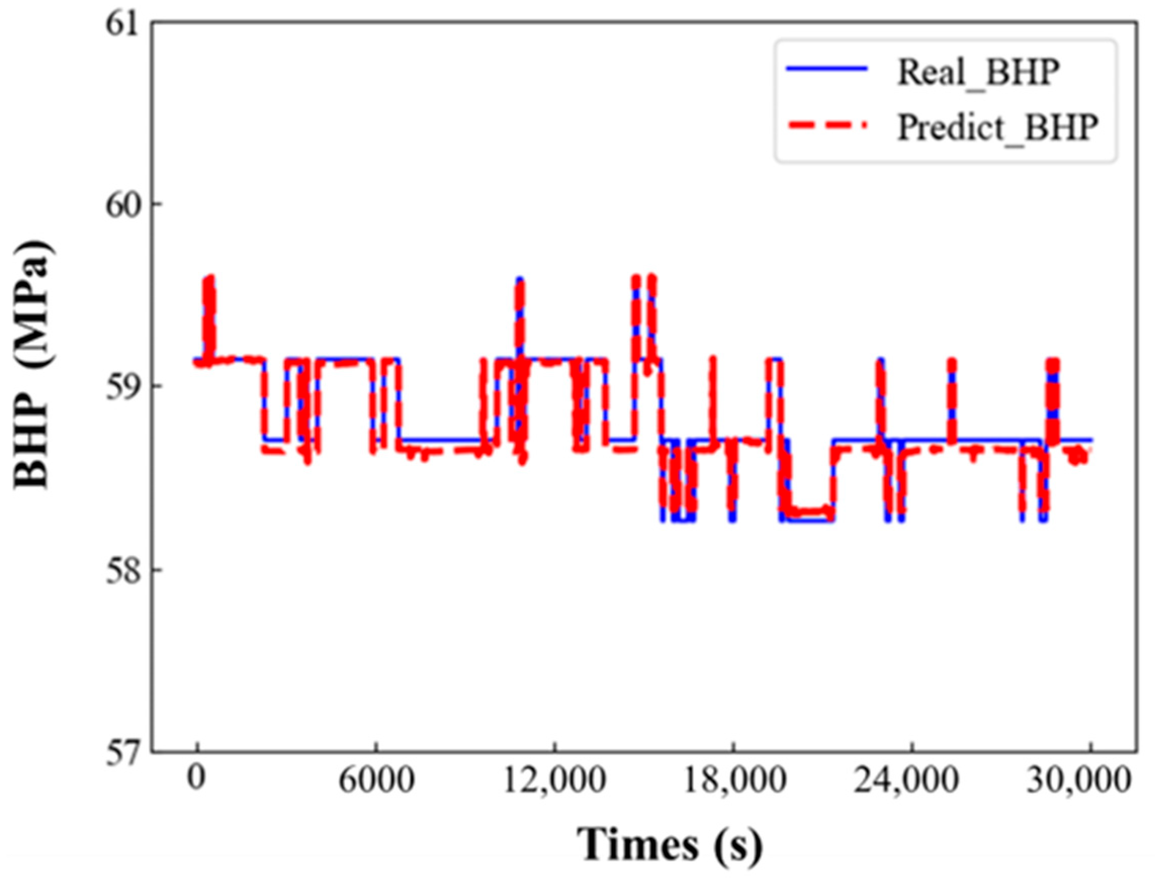
The field data test results demonstrate the effectiveness of the BHP prediction model based on the graph learning framework, presenting a robust alignment with actual BHP dynamics, as illustrated in Figure 4. The model exhibits a prompt response at the inflection point of pressure changes, indicating its capability to collectively extract parameter interactions through the adaptive graph layer. Furthermore, during pressure equilibrium, the model maintains a stable state. Although a slight deviation between the predicted pressure and the actual bottomhole pressure exists during the stabilization stage due to the influence of the activation function, this deviation is well within the acceptable engineering error range (5%).
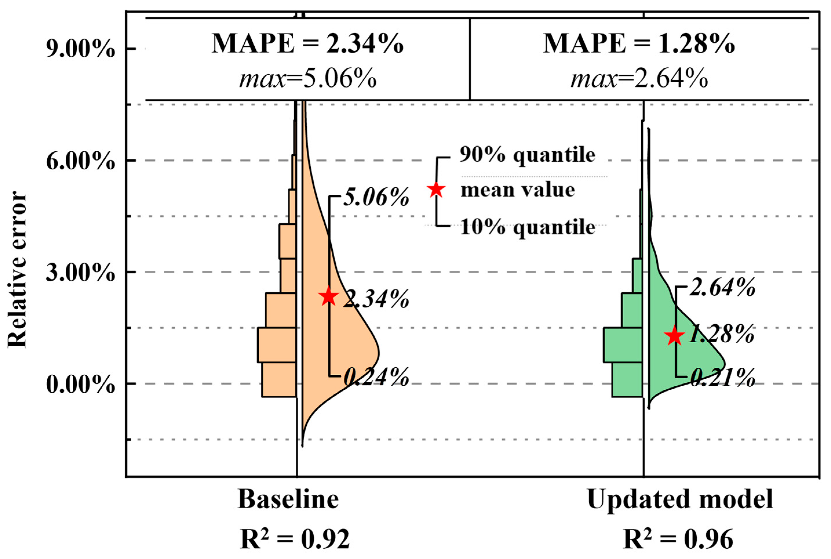
On this basis, the application scenario is simulated as a real-time data stream in the field, and the model is updated based on the incremental learning method. The comparative results, depicted in Figure 5, reveal that the incremental updating model achieves an MAPE of 1.28% and an R2 of 0.9563. This represents a notable enhancement compared to the original model, with a 45.3% reduction in MAPE and a 3.8% improvement in R2.

3.2. Model Interpretability

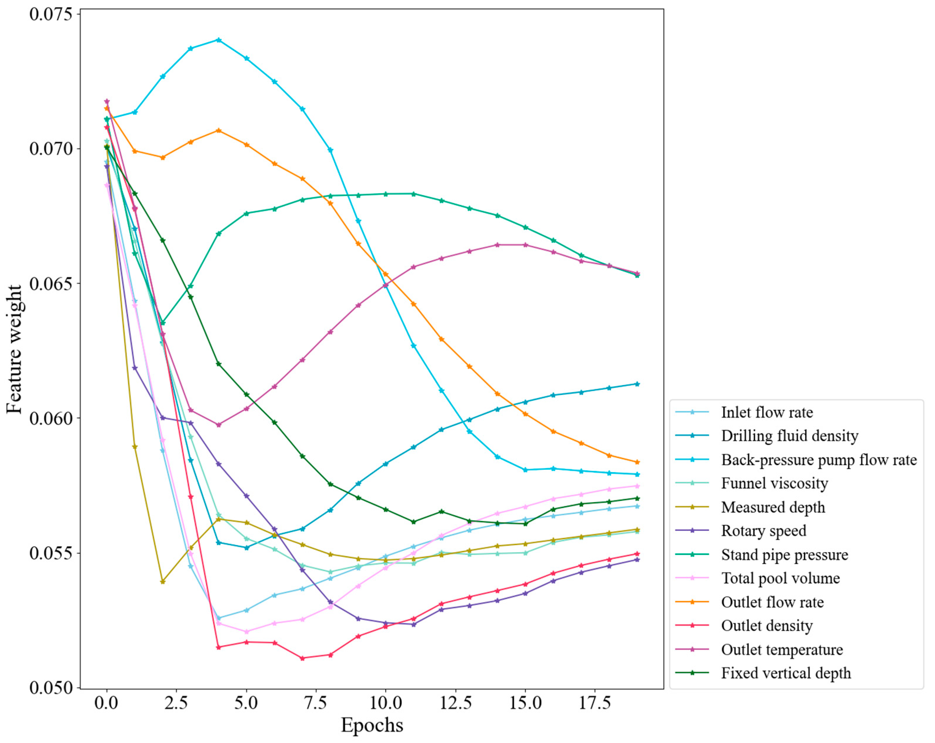
The temporal attention weights of the extraction model are illustrated in Figure 6. It is observed that the attention weights for all parameters tend to converge in the later stages of model training. Notably, the feature importance of rotary speed and outlet density exhibits a consistent upward trend, ultimately reaching peak values. The feature importance analysis indicates that the proposed model assigns the highest contribution to the inlet flow rate. For the datasets and operating conditions considered in this study, the inlet flow rate is the most informative parameter for BHP prediction. In particular, under abnormal drilling scenarios such as kicks, the outlet flow rate and other monitoring variables are known to play a paramount role, and the relative importance of features may change accordingly. Subsequently, the total pit volume, drilling fluid density, and standpipe pressure are ranked as relatively significant. Analysis suggests that fluctuations in the total pit volume reflect variations in the fluid volume within the wellbore. According to the principles of multiphase flow, the density of the drilling fluid determines the hydrostatic pressure in the wellbore. Under steady-state conditions, outlet temperature exerts negligible effects on bottomhole pressure variations. These results indicate that the proposed model not only achieves high prediction accuracy but also demonstrates reasonable interpretability.

3.3. Model Comparison

Moreover, in this section, to verify the validity of the IHGLN model, a model comparison test was conducted. Table 3 represents the six models that exhibit different performances in predicting the BHP. Notably, the IHGLN model outperforms the other four models, demonstrating the highest prediction accuracy. The simple architecture, the Multi-Layer Perceptron (MLP), shows the poorest performance with a significantly high MAPE of 15.36% and an R2 of 0.8894. This result indicates that simple feed-forward structures are fundamentally inadequate for capturing the complex, nonlinear, and sequential dynamics inherent in drilling time-series data. Among the advanced models, the CNN model fluctuates more drastically, with a maximum MAPE of 6.30%. The analysis suggests that the CNN pays more attention to the local feature changes, resulting in sudden changes at pressure inflection points. In contrast, the TCN and LSTM models focus extensively on the overall pressure trend while overlooking the changes at the inflection points, with the MAPE values of 4.0% and 4.1%, respectively. The CNN-LSTM model achieves an MAPE and an R2 of 2.93% and 0.9190. By combining the strengths of CNN in capturing local information and LSTM in capturing long-term information, the model demonstrates overall improvement. However, during the pressure stabilization phase, its stability falls short compared to the IHGLN model.

3.4. Ablation Study

To quantify the contributions of the core components to the IHGLN’s overall performance, an ablation study was conducted. We denote the IHGLN variants with different component configurations as follows:
  • IHGLN-w/o GL: Replacing the Graph Learning (GL) module with a fixed, identity adjacency matrix I.
  • IHGLN-w/LSTM: Replacing the TCN with a standard LSTM layer (maintaining similar parameter counts).
  • IHGLN-w/o Feature-Temporal Fusion: Simplifying the Feature Relationship Extraction Module by feeding the TCN output directly to the final Fully Connected layer.
The ablation results are summarized in Table 4. Replacing the Graph Learning module with a fixed identity matrix, removing dynamic feature relationship learning, resulted in the largest performance degradation, increasing the MAPE to 1.85%. This confirms that adaptive modeling of multivariate dependencies constitutes the most influential component of the architecture. Substituting the TCN Temporal Encoder with a conventional LSTM also produced a notable decline in performance, raising the MAPE to 1.76%, which underscores the advantage of dilated and causal convolutions in capturing long-range temporal dependencies in BHP sequences. Finally, directly feeding the TCN output into the prediction layer caused a moderate but meaningful degradation (MAPE = 1.51%). This indicates that, although the TCN and graph learning modules each contribute substantially, the explicit integration of relational graph information with temporal dynamics is indispensable for achieving optimal predictive accuracy.

4. Discussion

The proposed IHGLN offers distinct advantages for real-time BHP prediction by addressing core limitations of existing methods, while its applicability is tailored to industrial drilling scenarios and accompanied by clear avenues for improvement. Its primary strength lies in the explicit capture of parameter interaction mechanisms: unlike traditional models (e.g., LSTM, CNN-LSTM) that treat parameters as independent or implicitly model correlations, the IHGLN’s graph learning layer adaptively constructs a feature interaction graph to quantify pairwise and higher-order synergies, such as rotary speed-inlet flow rate driven flow regime transitions and drilling fluid density-outlet flow rate mediated hydrostatic-frictional coupling—that govern nonlinear BHP variations. This design directly translates to superior prediction accuracy, with a MAPE of 1.28% (25% lower than traditional intelligent models). In practical drilling engineering, downhole conditions (e.g., formation lithology, temperature gradients) drift constantly as depth increases. A static model trained on the initial section often fails to generalize to deeper sections due to distribution shifts. The proposed incremental updating workflow addresses this by utilizing a sliding window method. Despite the high accuracy, two key limitations must be acknowledged to ensure safe deployment. First, regarding the feature importance analysis, the model assigned low weights to Outlet Flow Rate, identifying Inlet Flow Rate as the dominant predictor. It must be clarified that this result is specific to “normal drilling conditions” where the system is in mass balance. The training dataset underwent outlier removal, effectively excluding kick or loss events. Therefore, while the model is excellent for predicting BHP under steady states, its current dismissal of Outlet Flow Rate makes it unsuitable for detecting kicks where the divergence between inlet and outlet flow is the primary indicator. Future iterations must incorporate specific “kick” scenarios into the training data to learn this critical safety logic. Second, the model’s robustness in well sections with highly variable solids content or extreme temperature gradients requires further validation with more diverse datasets.

5. Conclusions

(1) This paper introduces an approach by considering the mutual influence between parameters and the temporal sequence of BHP. It involves the construction of a graph learning layer, a temporal feature extraction module, and a feature relationship extraction module. These components characterize the association relationship between input parameter nodes, facilitating data-driven graph learning to enhance the accuracy of the model predictions.
(2) We propose a real-time BHP prediction model based on the improved graph learning network. The model’s hyperparameters are carefully selected using a Bayesian optimization algorithm. The sliding window method is employed to achieve incremental learning of the model in real-time data streams, thereby enhancing the feasibility of on-the-ground applications.
(3) Field data application demonstrates the significant advantage of the proposed IHGLN model in prediction compared to four other deep learning models. The IHGLN model achieves an average error MAPE of 1.28% and exhibits good stability and accuracy.
In the future, the proposed IHGLN model exhibits good scalability and deployment potential in field operations. Firstly, the adaptive graph learning mechanism enables the model to adjust to variable drilling environments, which supports its extension to different formations and operational conditions. Secondly, the trained model can be efficiently transferred to new wells with limited labeled data through parameter fine-tuning, reducing the cost of retraining from scratch. Finally, with its lightweight temporal convolution structure and real-time computational efficiency, the model can be integrated into intelligent drilling monitoring systems to provide continuous BHP prediction and early warning during drilling operations. Future work will focus on multi-well and multi-condition validation, as well as implementing the model into site-level digital platforms for closed-loop drilling control.

Author Contributions

Conceptualization, Z.P. and R.Z.; methodology, R.Z.; software, R.Z.; validation, Z.P., M.M., and H.W.; formal analysis, Q.L. and C.W.; investigation, Z.P. and M.M.; resources, H.W.; data curation, Z.P.; writing—original draft preparation, R.Z.; writing—review and editing, Z.P. and Q.L.; visualization, M.M., Q.L., and C.W.; supervision, H.W.; project administration, H.W.; funding acquisition, Z.P. All authors have read and agreed to the published version of the manuscript.

Funding

This research was funded by the National Natural Science Foundation of China, grant number 52421002, the Science Foundation of China University of Petroleum, Beijing, grant number 2462023QNXZ01, and the Distinguished Young Foundation of National Natural Science Foundation of China, grant number 5212540.

Data Availability Statement

The original contributions presented in this study are included in the article. Further inquiries can be directed to the corresponding authors.

Conflicts of Interest

Author Zhaoyu Pang was employed by the CNOOC Research Institute Co., Ltd. The remaining authors declare that the research was conducted in the absence of any commercial or financial relationships that could be construed as a potential conflict of interest.

Abbreviations

The following abbreviations are used in this manuscript:
BHPBottomhole pressure
ANNArtificial neural network
IHGLNImproved hybrid graph learning network
ConvConvolution
TCNTemporal convolutional network
CNNConvolutional neural network
LSTMLong short-term memory
MAPEMean absolute percentage error
R2Coefficient of determination

References

  1. Zhang, C.; Zhang, R.; Zhu, Z.; Song, X.; Su, Y.; Li, G.; Han, L. Bottom Hole Pressure Prediction Based on Hybrid Neural Networks and Bayesian Optimization. Pet. Sci. 2023, 20, 3712–3722. [Google Scholar] [CrossRef]
  2. Li, G.; Song, X.; Tian, S.; Zhu, Z. Intelligent Drilling and Completion: A Review. Engineering 2022, 18, 33–48. [Google Scholar] [CrossRef]
  3. Wang, Z.; Gao, D.; Liu, J. Multi-Objective Sidetracking Horizontal Well Trajectory Optimization in Cluster Wells Based on DS Algorithm. J. Pet. Sci. Eng. 2016, 147, 771–778. [Google Scholar] [CrossRef]
  4. Zheng, J.; Lu, C.; Gao, L. Multi-Objective Cellular Particle Swarm Optimization for Wellbore Trajectory Design. Appl. Soft Comput. 2019, 77, 106–117. [Google Scholar] [CrossRef]
  5. Duan, S.; Song, X.; Cui, Y.; Xu, Z.; Liu, W.; Fu, J.; Zhu, Z.; Li, D. Intelligent Kick Warning Based on Drilling Activity Classification. Geoenergy Sci. Eng. 2023, 222, 211408. [Google Scholar] [CrossRef]
  6. Duan, S.; Song, X.; Xu, Z.; Zhou, M.; Zhu, Z.; Yao, X.; Hemmati, A.; Verma, S. Wellbore Pressure Inversion Model Based on Wavelet Analysis During Gas Kick. SPE J. 2025, 30, 3416–3436. [Google Scholar] [CrossRef]
  7. Tariq, Z.; Mahmoud, M.; Abdulraheem, A. Real-Time Prognosis of Flowing Bottom-Hole Pressure in a Vertical Well for a Multiphase Flow Using Computational Intelligence Techniques. J. Pet. Explor. Prod. Technol. 2020, 10, 1411–1428. [Google Scholar] [CrossRef]
  8. Hu, S.; Sheng, M.; Shi, S.; Li, J.; Tian, S.; Li, G. Optimization of Fracturing Stages/Clusters in Horizontal Well Based on Unsupervised Clustering of Bottomhole Mechanical Specific Energy on the Bit. Nat. Gas Ind. B 2023, 10, 583–590. [Google Scholar] [CrossRef]
  9. Zhang, R.; Zhu, Z.; Song, X.; Li, G.; Wang, B.; Zhang, C.; Wang, C. A Knowledge-Guided Temporal Graph Neural Network for Predicting Rate of Penetration in Complex Formations. SPE J. 2025, 1–20. [Google Scholar] [CrossRef]
  10. Opoku, D.; Al-Ghamdi, A.; Osei, A. Novel Method to Estimate Bottom Hole Pressure in Multiphase Flow Using Quasi-Monte Carlo Method. In Proceedings of the International Petroleum Technology Conference (IPTC), Dhahran, Saudi Arabia, 13–14 January 2020; p. D021S050R001. [Google Scholar] [CrossRef]
  11. Okoro, E.E.; Obomanu, T.; Sanni, S.E.; Olatunji, D.I.; Igbinedion, P. Application of Artificial Intelligence in Predicting the Dynamics of Bottom Hole Pressure for Under-Balanced Drilling: Extra Tree Compared with Feed Forward Neural Network Model. Petroleum 2022, 8, 227–236. [Google Scholar] [CrossRef]
  12. Zhang, R.; Song, X.; Li, G.; Lv, Z.; Zhu, Z.; Zhang, C.; Gong, C. A Novel Hybrid Transfer Learning Method for Bottom Hole Pressure Prediction. In Proceedings of the ASME 2023 42nd International Conference on Ocean, Offshore and Arctic Engineering (OMAE 2023), Melbourne, Australia, 11–16 June 2023; Volume 9: Offshore Geotechnics; Petroleum Technology. [Google Scholar] [CrossRef]
  13. Hu, G.; Xiao, X.; Shen, M.; Zhang, B.; Yan, X.; Liu, Y. TCGNN: Packet-Grained Network Traffic Classification via Graph Neural Networks. Eng. Appl. Artif. Intell. 2023, 123, 106531. [Google Scholar] [CrossRef]
  14. Kim, J.; Kim, T.; Ryu, J.-G.; Kim, J. Spatiotemporal Graph Neural Network for Multivariate Multi-Step Ahead Time-Series Forecasting of Sea Temperature. Eng. Appl. Artif. Intell. 2023, 126, 106854. [Google Scholar] [CrossRef]
  15. Wang, S.; Li, Y.; Zhang, J.; Meng, Q.; Meng, L.; Gao, F. PM2.5-GNN: A Domain Knowledge Enhanced Graph Neural Network for PM2.5 Forecasting. In Proceedings of the 28th International Conference on Advances in Geographic Information Systems, Seattle, WA, USA, 3–6 November 2020; pp. 163–166. [Google Scholar] [CrossRef]
  16. Zolfagharroshan, M.; Khamehchi, E. Accurate Artificial Intelligence-Based Methods in Predicting Bottom-Hole Pressure in Multiphase Flow Wells, a Comparison Approach. Arab. J. Geosci. 2021, 14, 284. [Google Scholar] [CrossRef]
  17. Lehmann Rüdiger 3σ-Rule for Outlier Detection from the Viewpoint of Geodetic Adjustment. J. Surv. Eng. 2013, 139, 157–165. [CrossRef]
  18. Zhang, C.; Song, X.; Liu, Z.; Ma, B.; Lv, Z.; Su, Y.; Li, G.; Zhu, Z. Real-Time and Multi-Objective Optimization of Rate-of-Penetration Using Machine Learning Methods. Geoenergy Sci. Eng. 2023, 223, 211568. [Google Scholar] [CrossRef]
  19. Yin, H.; Zhao, X.; Li, Q. Research on Adaptive Prediction Model of Rate of Penetration under Dynamic Formation Conditions. Eng. Appl. Artif. Intell. 2024, 133, 108281. [Google Scholar] [CrossRef]
  20. Lea, C.; Vidal, R.; Reiter, A.; Hager, G.D. Temporal Convolutional Networks: A Unified Approach to Action Segmentation. In Proceedings of the Computer Vision—ECCV 2016 Workshops; Hua, G., Jégou, H., Eds.; Springer International Publishing: Cham, Switzerland, 2016; pp. 47–54. [Google Scholar] [CrossRef]
  21. Akiba, T.; Sano, S.; Yanase, T.; Ohta, T.; Koyama, M. Optuna: A Next-Generation Hyperparameter Optimization Framework. In Proceedings of the 25th ACM SIGKDD International Conference on Knowledge Discovery & Data Mining, Anchorage, AK, USA, 4–8 August 2019; pp. 2623–2631. [Google Scholar] [CrossRef]
  22. Hochreiter, S.; Schmidhuber, J. Long Short-Term Memory. Neural Comput. 1997, 9, 1735–1780. [Google Scholar] [CrossRef] [PubMed]
  23. O’Shea, K.; Nash, R. An Introduction to Convolutional Neural Networks. arXiv 2015. [Google Scholar] [CrossRef]
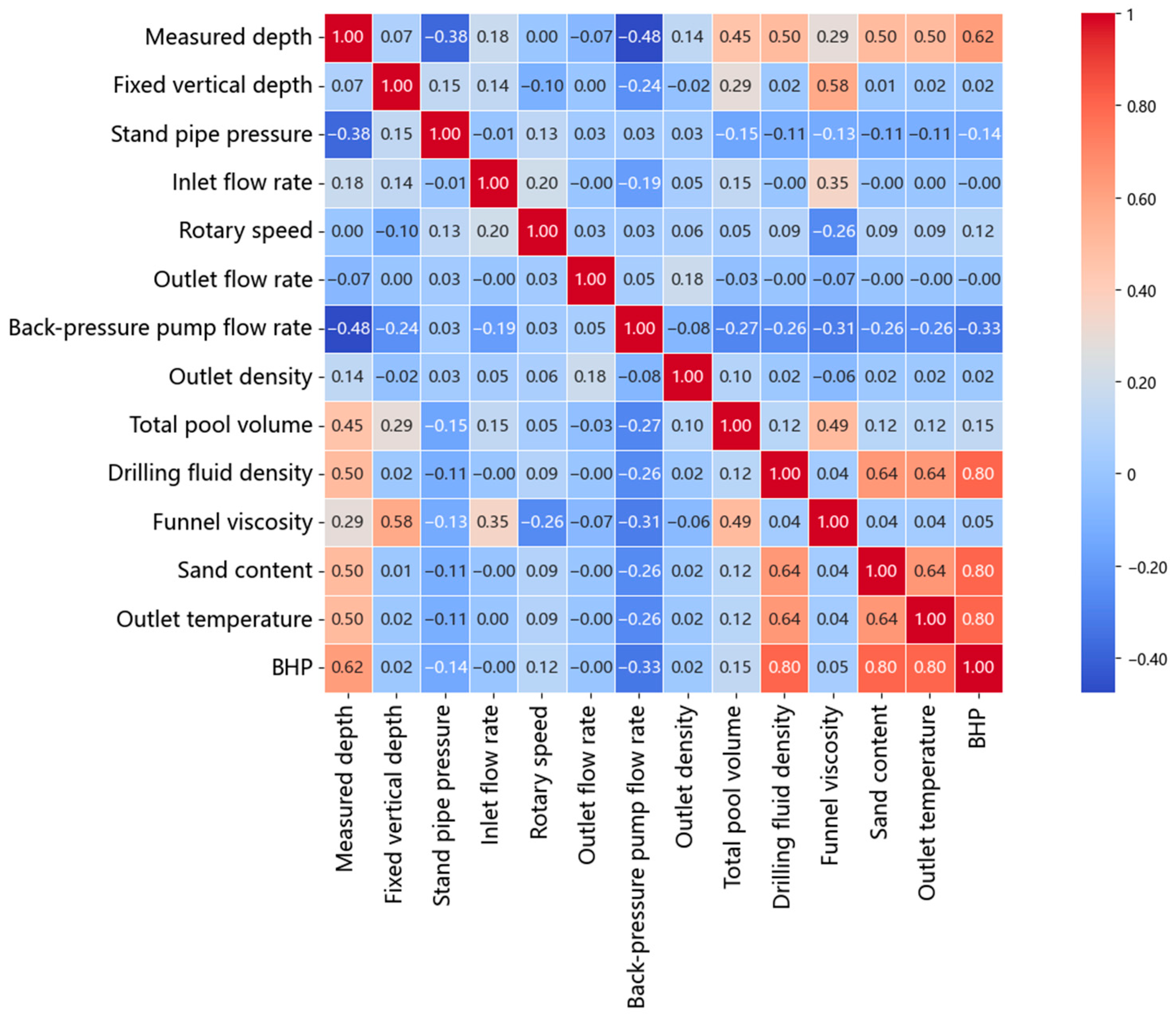
Figure 1. Correlation matrix thermal diagram.
Processes 13 04081 g001
Figure 2. The structure of the proposed IHGLN model.
Processes 13 04081 g002
Figure 3. The sliding window method in incremental updating.
Processes 13 04081 g003
Figure 4. Comparison of predicted BHP and measured BHP.
Processes 13 04081 g004
Figure 5. Comparison of BHP predictions of incremental and non-incremental updates. The red five-pointed star represents the mean value of relative errors.
Processes 13 04081 g005
Figure 6. Temporal attention weights in different epochs.
Processes 13 04081 g006
Table 1. The statistical description of datasets.
Measured Depth (m)Fixed Vertical Depth (m)Stand Pipe Pressure (MPa)Inlet Flow Rate (L/s)Rotary Speed (rpm)Outlet Flow Rate (L/s)Back-Pressure Pump Flow Rate (L/s)
Mean6087.994935.3919.3713.7511.6813.748.84
Min5832.824930.1516.5413.306.2813.406.78
Max6705.784942.0722.1719.4723.5019.4710.78
Outlet Density (g/cm3)Total Pool Volume (m3)Drilling Fluid Density (g/cm3)Outlet Temperature ()Funnel Viscosity (s)Sand Content (%)BHP (MPa)
Mean1.19146.441.151440.258.58
Min1.17124.381.150430.256.94
Max1.82175.231.252450.259.58
Table 2. Hyperparameter configurations. Here, “Channels” denotes the number of convolutional filters in each TCN block. “Fully connected neurons” is the number of hidden units in each layer of the final multilayer perceptron.
HyperparameterOptimal Values
Channels(16, 32, 64)
Fully connected neurons(8, 16, 32, 64)
Dropout(0.1, 0.2, 0.3)
Learning rate(0.01, 0.001, 0.0001)
Epoch(50, 80, 100)
Table 3. Evaluation metrics of five models.
ModelMAPE (%)R2
IHGLN1.28 ± 0.030.9563 ± 0.0031
MLP15.36 ± 0.130.8894 ± 0.0043
CNN8.30 ± 0.080.8572 ± 0.0056
LSTM4.12 ± 0.060.8991 ± 0.0039
TCN4.01 ± 0.050.9013 ± 0.0032
CNN-LSTM2.93 ± 0.030.9190 ± 0.0032
Table 4. The results of ablation study.
ModelsMAPE (%)R2
w/o GL1.850.9320
w/LSTM1.510.9450
w/o Feature-Temporal Fusion1.760.9365
IHGLN1.280.9563
Disclaimer/Publisher’s Note: The statements, opinions and data contained in all publications are solely those of the individual author(s) and contributor(s) and not of MDPI and/or the editor(s). MDPI and/or the editor(s) disclaim responsibility for any injury to people or property resulting from any ideas, methods, instructions or products referred to in the content.