An Optimized CNN-BiLSTM-RF Temporal Framework Based on Relief Feature Selection and Adaptive Weight Integration: Rotary Kiln Head Temperature Prediction

Abstract

The kiln head temperature of a rotary kiln is a core process parameter in cement clinker production, and its accurate prediction coupled with uncertainty quantification is crucial for process optimization, energy consumption control, and safe operation. To tackle the prediction challenges arising from strong multi-variable coupling and nonlinear time series characteristics, this paper proposes a prediction approach integrating feature selection, heterogeneous model ensemble, and probabilistic interval estimation. Firstly, the Relief algorithm is adopted to select key features and construct a time series feature set with high discriminability. Then, a hierarchical architecture encompassing deep feature extraction, heterogeneous model fusion, and probabilistic interval quantification is devised. CNN is utilized to extract spatial correlation features among multiple variables, while BiLSTM is employed to bidirectionally capture the long-term and short-term temporal dependencies of the temperature sequence, thereby forming a deep temporal–spatial feature representation. Subsequently, RF is introduced to establish a heterogeneous model ensemble mechanism, and dynamic weight allocation is implemented based on the Mean Absolute Error of the validation set to enhance the modeling capability for nonlinear coupling relationships. Finally, Gaussian probabilistic regression is leveraged to generate multi-confidence prediction intervals for quantifying prediction uncertainty. Experiments on the real rotary kiln dataset demonstrate that the R² of the proposed model is improved by up to 15.5% compared with single CNN, BiLSTM and RF models, and the Mean Absolute Error is reduced by up to 27.7%, which indicates that the model exhibits strong robustness to the dynamic operating conditions of the rotary kiln and provides both accuracy guarantee and risk quantification basis for process decision-making. This method offers a new paradigm integrating feature selection, adaptive heterogeneous model collaboration, and uncertainty quantification for industrial multi-variable nonlinear time series prediction, and its hierarchical modeling concept is valuable for the intelligent perception of complex process industrial parameters.

1. Introduction

With the continuous improvement of industrial intelligence levels, smart manufacturing technology has become the core driving force for promoting the transformation and upgrading of traditional manufacturing industries [1]. As a typical process industry, cement manufacturing relies heavily on the accurate control of the kiln head temperature of the rotary kiln during its production process, which is directly related to the stability of the calcination process, the consistency of clinker quality, and the optimization of system energy efficiency. Therefore, implementing real-time monitoring and dynamic optimal control of the kiln head temperature is of crucial significance for improving enterprise production efficiency and realizing closed-loop management of smart manufacturing.

Currently, the modeling methods for the operation process of rotary kilns are mainly divided into two categories: numerical simulation and data-driven methods [2,3]. Numerical simulation methods are based on the principles of heat transfer, dynamics, and thermodynamics. They discretize the internal space of the kiln into grid units, establish and solve combustion models, drying models, and mass balance models [4,5,6]. Although this method can calculate the kiln head temperature with high precision, the production process of the rotary kiln involves processes such as gas–solid two-phase flow, pulverized coal combustion, and unsteady heat transfer, which exhibit strong nonlinearity, large time delay, and strong multi-variable coupling characteristics [7,8]. These characteristics result in substantial computational resources required for model solving and a long convergence time, making it difficult to meet the requirements of real-time monitoring.

Data-driven modeling methods can establish mathematical models for the rotary kiln operation process by learning from the historical operational data of rotary kilns using machine learning techniques. Yin et al. [9] proposed an adaptive data-driven soft sensor method: by integrating moving window technology and the just-in-time learning (JITL) mechanism into the partial least squares regression (PLSR) algorithm, they developed two adaptive soft sensors for real-time monitoring and prediction of the zinc rotary kiln temperature. This method effectively copes with dynamic temperature changes and eliminates the time delay issue of traditional models. Wang et al. [10] put forward a rotary kiln temperature field prediction method that combines computational fluid dynamics (CFDs) with machine learning. They generated a dataset covering 625 operating conditions via CFD to train the prediction model; while maintaining prediction accuracy, this method reduced the computation time from 2 to 3 weeks (of traditional methods) to 10 s, with a significant decrease in prediction error.

Zheng et al. [11] proposed an optimization method for NO_x emissions in the cement calcination process based on improved just-in-time learning Gaussian mixture regression (JITL-GMR). By optimizing sample selection through a spatiotemporal similarity strategy and combining the particle swarm optimization (PSO) algorithm to dynamically optimize operating parameters, this method significantly reduced the NO_x emission level at the kiln tail. Although the aforementioned methods can describe the rotary kiln operation process to a certain extent, they fail to capture deep-seated features due to the inherent limitations of traditional machine learning [12]. Consequently, they exhibit poor learning capabilities for the process data of rotary kilns, which are characterized by strong nonlinearity and long time delays.

With the development of deep learning [13] technology, this approach has attracted the attention of numerous researchers. Deep learning can capture deep-seated features through large-scale datasets and thereby construct corresponding mathematical models, and it has been widely applied in various industrial production processes [14,15,16]. In terms of rotary kiln monitoring, Zheng et al. [17] proposed a hybrid modeling strategy integrating process mechanism and recurrent neural networks (RNNs). By compensating for the residence time inside the kiln through a time-delay mechanism and introducing attention mechanism-enhanced long short-term memory (LSTM) networks to capture nonlinear time-varying characteristics, this strategy significantly improved the accuracy and robustness of dynamic modeling for cement rotary kilns. Xu et al. [18] developed a graph neural network (GNN) model. By optimizing unstructured grid computation using the Cleary–Luby–Jones–Plassmann graph topology coarsening algorithm, this model maintained high precision in predicting the two-dimensional temperature field of the rotary kiln while improving computational efficiency by three orders of magnitude compared with traditional CFD methods. Thus, it provides a new approach for real-time temperature monitoring and energy efficiency optimization of rotary kilns. Li et al. [19] proposed a multi-parameter collaborative optimization method based on data-driven models and improved particle swarm optimization (PSO) algorithms. By using a sparse autoencoder-based bidirectional LSTM network to predict combustion status and NO_x emissions, this method achieved high stability and low-cost control of NO_x emissions during waste incineration. Wang et al. [20] constructed a time series prediction model (nonlinear autoregressive with exogenous inputs-time convolutional network, NARX-TCN) that integrates inlet flue gas, process control parameters, and pollutants. By dynamically predicting the next-moment SO₂ concentration through nonlinear autoregression and time convolutional networks, and by reducing the flue gas pressure at the absorber inlet or increasing the pressure in the concentration section, this model effectively improved desulfurization efficiency and provided a data-driven solution for real-time regulation of industrial parameters.

To address the challenges of strong multi-variable coupling and temporal dynamic prediction for the clinker rotary kiln head temperature, this paper proposes a heterogeneous ensemble model integrating Relief feature selection and optimized CNN-BiLSTM-RF. By leveraging multi-variable feature selection and an adaptive error-oriented weight fusion mechanism, the model enhances prediction robustness, providing a new paradigm for temporal prediction of complex industrial time series parameters. The main innovations of this paper are as follows:

(1) A Relief multi-variable feature selection method adapted to industrial scenarios is proposed. Based on multi-source parameters of the rotary kiln, the method calculates the contribution of features to the differences in target values of neighboring samples. It screens out high-contribution features, effectively filtering noise and temporal redundant information, improving the discriminability of input features, and enhancing the model’s anti-interference capability from the data source.

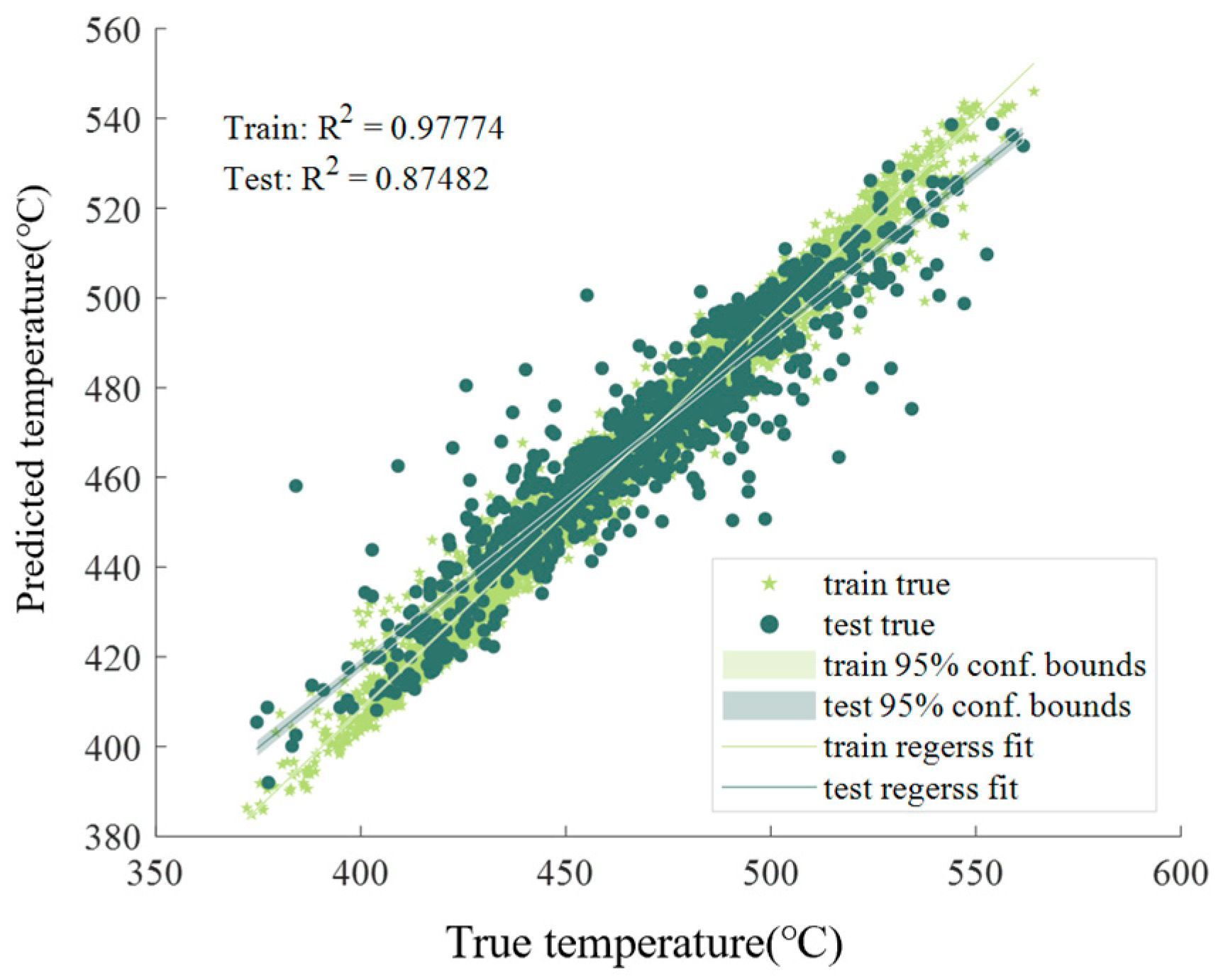
(2) A three-layer heterogeneous ensemble architecture of CNN-BiLSTM-RF is constructed. CNN-BiLSTM extracts spatial coupling features of multiple variables and captures bidirectional temporal dependencies, taking both historical influences and future trends into account. Meanwhile, RF performs dynamic decision-making based on feature weights, overcoming the limitations of single models. The R² of the proposed model on the test set reaches 0.87482, representing an increase of up to 15.5% compared with single models.

(3) Gaussian probabilistic intervals are constructed to achieve reasonable quantification of uncertainty, supporting reliable future trend prediction and thus providing a basis for decision-making.

The temporal forecasting model proposed in this study holds broad application potential in industrial scenarios. For general industrial time series forecasting tasks—such as predicting parameters in chemical reaction processes, monitoring equipment status in smart manufacturing, and forecasting loads in energy systems—the integrated feature selection, Variational Mode Decomposition (VMD) denoising, and adaptive weighted fusion strategies effectively address common challenges in industrial data, including high noise levels, feature redundancy, and nonlinear correlations. By accurately capturing both spatial correlations and bidirectional temporal dependencies in time series data, the model provides reliable support for real-time industrial process control, fault warning, and optimized decision-making. This contributes to reducing energy consumption, improving product quality consistency, and offers valuable technical references for intelligent industrial upgrading.

2. Data Preprocessing and Feature Engineering

2.1. Data Description

Experimental data were obtained from the rotary kiln control system of a cement manufacturing enterprise. The input data include 6 variables, namely rotary kiln current, rotary kiln rotation speed, tertiary air temperature, raw meal feed rate, flue chamber temperature, and actual coal feed rate at the kiln head; the output data is the kiln head temperature. The dataset was divided into a training set, validation set, and test set in a ratio of 7:2:1. The dataset comprises a total of 8483 samples, divided into 5938 for training, 1697 for validation, and 848 for testing. The split was performed sequentially according to the temporal order of data collection (i.e., non-random splitting): the first 70% of the data were allocated to the training set, the subsequent 20% to the validation set, and the final 10% to the test set. This approach preserves the temporal dependencies inherent in industrial time series data and helps prevent data leakage.

The key hyperparameters include a hidden layer size of 32 neurons, a learning rate of 0.001, 70 training epochs, and a batch size of 851.

All experiments were conducted on a CPU-based computing environment (Intel Core i5-13500H, 2.6 GHz, 16 GB RAM) using MATLAB 2023b as the running platform.

2.2. Data Preprocessing

2.2.1. Missing Value Handling

Interpolation was employed to address missing values, and specifically, spline interpolation was adopted. After identifying the positions of missing values, the missing values were removed while valid data and their corresponding position indices were retained. Finally, spline interpolation was used to fill the vacant positions, resulting in the final processed data. The formula is as follows:

$$S(x)=\left\{\begin{array}{l}{a}_1{x}^3+b_1{x}^2+c_{1}x+d_1,x\in [x_1,x_2]\\ a_2{x}^3+b_2{x}^2+c_{2}x+d_2,x\in [x_2,x_3]\\ ⋮\\ a_{n-1}{x}^3+b_{n-1}{x}^2+c_{n-1}x+d_{n-1},x\in [x_{n-1},x_n]\end{array}\right.$$

(1)

where $a_i,b_i,c_i,d_i(i=1,2,\dots ,n-1)$ is the cubic polynomial coefficient of each interval, and it satisfies:

The function value is continuous:

$$S(x_i^{+})=S(x_i^{-})=y_i,(i=2,\dots ,n-1)$$

(2)

The first derivative is continuous:

$$S^{\prime }(x_i^{+})=S^{\prime }(x_i^{-}),(i=2,\dots ,n-1)$$

(3)

The second derivative is continuous:

$$S^{″}(x_i^{+})=S^{″}(x_i^{-}),(i=2,\dots ,n-1)$$

(4)

Natural spline boundary conditions:

$$S^{″}(x_1)=S^{″}(x_n)=0$$

(5)

Through spline interpolation, the values at missing positions are estimated smoothly based on the trends of valid data points, ultimately yielding a complete, continuous dataset free of missing values. Compared with simple linear interpolation, this method better preserves the inherent trends and smoothness of the data—an advantage that is particularly critical for maintaining the temporal continuity and dynamic characteristics of rotary kiln operational data.

2.2.2. Data Standardization

To mitigate the impact of inconsistent dimensions of different variables on model performance, the Z-score converts the data into a distribution with a mean of 0 and a standard deviation of 1. The formula is given as follows:

$$z={\displaystyle \frac{x-\mu }{\sigma }}$$

(6)

where $z$ represents the standardized value, $x$ is the original value, $\mu$ is the average value of the feature, and $\sigma$ is the standard deviation of the feature.

By eliminating differences in dimensions and units among various variables, the data are standardized to share the same scale and dimension. This standardization process facilitates more effective comparison and analysis of multi-variable data, while also preventing variables with larger magnitudes from dominating the model training process—an issue that could otherwise distort the learning of feature correlations.

2.3. Feature Engineering

2.3.1. Time Sliding Window Feature Extraction

The time sliding window technique was adopted, with a historical feature step size of 2, a historical sequence step size of 10, a number of prediction points of 12, a window size of 32, and a step length of 1. For each variable, statistical features and time series features were extracted; through sliding window processing, the original single-time-point data were converted into feature vectors containing historical temporal information. This transformation enables the model to capture the dynamic evolutionary patterns of variables over time, laying a foundation for subsequent temporal dependency modeling.

2.3.2. Feature Selection

Relief is a classic instance-based feature selection algorithm. Its core lies in screening features by measuring their predictive contribution to continuous target values among neighboring samples, making it particularly suitable for time series or regression datasets with noisy and redundant features. The core logic is as follows: for each sample, neighboring samples in the feature space are identified; by calculating the differences in target values between these neighboring samples and the current sample with respect to the target feature, the explanatory power of the feature for the target value is evaluated. The formula is given as follows:

$$w_j=w_j-{\displaystyle \frac{1}{2mk}}{\displaystyle {\sum }_{i=1}^m{\displaystyle {\sum }_{l=1}^k(diff(x_i^j,N_{i,l}^j)\cdot diff(y_i,y_{N_{i,l}}))}}$$

(7)

where $y_i$ is the continuous target value of sample $x_i$; $N_{i,l}$ is the l-th nearest neighbor of sample $x_i$; $diff(y_i,y_{N_{i,l}})=\left|y_i-y_{N_{i,l}}\right|$ is the absolute difference in the target value; $diff(x_i^j,N_{i,l}^j)=\left|x_i^j-N_{i,l}^j\right|$ is the absolute difference in feature $j$.

Leveraging this difference correlation-based evaluation mechanism, Relief can effectively capture nonlinear correlations between features and continuous target variables. This not only filters out irrelevant and redundant information but also provides a high-discriminability input feature set for the subsequent temporal prediction model, thereby enhancing the model’s learning efficiency and generalization performance.

3. Optimized CNN-BiLSTM-RF Time Series Framework

3.1. Overall Model Architecture

The optimized CNN-BiLSTM-RF model is mainly composed of two parts: a deep feature extraction layer (CNN-BiLSTM) and a dynamic decision fusion layer (RF), and is optimized using the metaheuristic algorithm. Specifically, the CNN-BiLSTM module consists of an input layer, convolutional layer, batch normalization layer, ReLU activation layer, max-pooling layer, Flatten layer, BiLSTM layer, fully connected layer, and regression output layer.

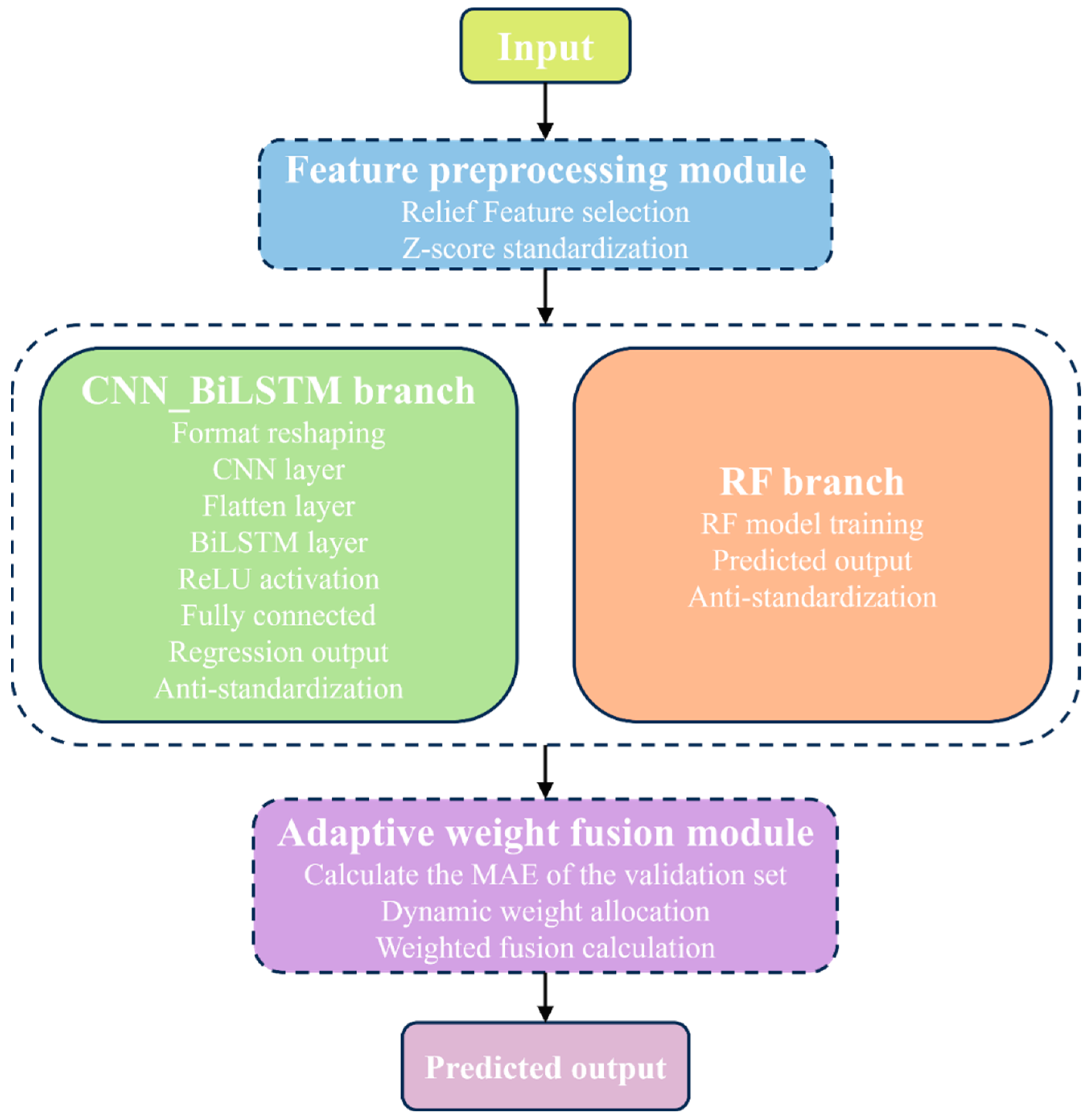
Unlike traditional machine learning models such as XGBoost [21], the proposed overall model adopts a phased modeling approach, coordinating parameters of multiple modules to perform feature extraction and time series modeling. The architecture of the overall model is illustrated in Figure 1.

Feature Preprocessing Module: The input data first undergoes Relief feature selection to identify and retain core features strongly relevant to the prediction target. Subsequently, Z-score normalization is applied to eliminate the influence of varying measurement scales.

CNN_BiLSTM Branch: The processed data is reshaped to fit the convolutional input requirements. A CNN layer is employed to extract local spatial correlations and short-term patterns. The resulting feature maps are then flattened and fed into a BiLSTM layer to capture bidirectional long-term temporal dependencies. The output is passed through a ReLU activation function and a fully connected layer for regression, followed by denormalization to restore the original data scale.

RF Branch: A Random Forest model is trained directly on the preprocessed data. Its predictions are similarly denormalized to the original scale.

Adaptive Weight Fusion Module: The Mean Absolute Error (MAE) of each branch on the validation set is calculated. Fusion weights for the two branches are dynamically assigned based on the inverse of their respective MAE values, favoring the more reliable branch. The final prediction is obtained as the weighted sum of the two branches’ outputs.

Prediction Output Module: This module delivers the adaptively fused final prediction.

3.2. Adaptive Weight Allocation Mechanism

After initializing the optimized hyperparameters, setting the upper and lower bounds of the optimized parameters, and determining the number of optimization iterations, the meta-heuristic optimizer MMGO (Mapping mountain gazelle optimizer) algorithm [22] was used to search for the optimal hyperparameters of the model. Subsequently, the errors of the two sub-models (CNN-BiLSTM and RF) on the validation set were recorded, and the relative error difference ${\Delta }_r$ was employed to evaluate the performance of different sub-models. The corresponding formula is as follows:

$${\Delta }_r={\displaystyle \frac{\left|E_{CB}-E_{RF}\right|}{\max (E_{CB},E_{RF})}}$$

(8)

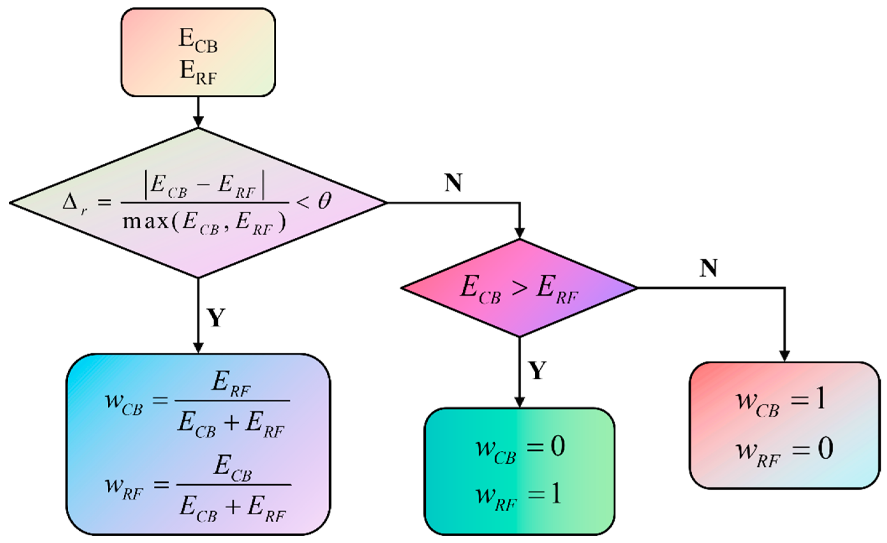
The Mean Absolute Error (MAE) of CNN-BiLSTM and RF on the validation set was calculated to ensure that weight allocation was based on model generalization ability rather than the fitting effect on the training set. Then, the appropriate weights were selected and allocated by judging the errors of the two sub-models on the validation set. The allocation process is shown in Figure 2.

In Figure 2, $E_{CB}$ represents the MAE of the CNN-BiLSTM model, $E_{RF}$ denotes the MAE of the Random Forest model, $W_{CB}$ refers to the weight assigned to the CNN-BiLSTM model, $W_{RF}$ indicates the weight assigned to the Random Forest model, and $\theta$ is the decision threshold, which is set to 0.1 in this study.

After calculating $E_{CB}$ and $E_{RF}$, their absolute difference is compared against the threshold $\theta$. If the difference is less than or equal to $\theta$, the weights $W_{CB}$ and $W_{RF}$ are allocated proportionally based on the respective errors. Conversely, if the difference exceeds $\theta$, the model with the smaller error is assigned full weight, effectively disregarding the model with the larger error.

After weight allocation, the de-normalized predicted values of the two sub-models were weighted and summed according to the allocated weights to obtain the final prediction result. Dynamically allocating the weights of the two sub-models based on relative error differences to achieve advantage complementarity is the key feature that distinguishes this model from traditional single models.

3.3. Loss Function

For CNN-BiLSTM, to avoid the impact of extreme deviations on its performance, special attention needs to be paid to the stable convergence of the model itself. Therefore, the mean square error (MSE) is adopted as its loss function, and the formula is as follows:

$$L_{C{B}_{MSE}}={\displaystyle \frac{1}{N}}{{\displaystyle {\sum }_{i=1}^N(y_i-{\widehat{y}}_i)}}^2$$

(9)

where $N$ represents the sample size, $y_i$ is the true value of the i-th sample, ${\widehat{y}}_i$ is the model prediction value of the i-th sample.

However, as a decision tree-based ensemble model, RF requires greater focus on the overall characteristics of the data. The MAE imposes a linear penalty on outliers, which better facilitates minimizing the error of child nodes and thus improves model performance. Consequently, MAE is selected as the loss function for RF, with the formula given below:

$$L_{R{F}_{MAE}}={\displaystyle \frac{1}{N}}{\displaystyle {\sum }_{i=1}^N\left|y_i-{\widehat{y}}_i\right|}$$

(10)

where $N$ represents the sample size, $y_i$ is the true value of the i-th sample, ${\widehat{y}}_i$ is the model prediction value of the i-th sample.

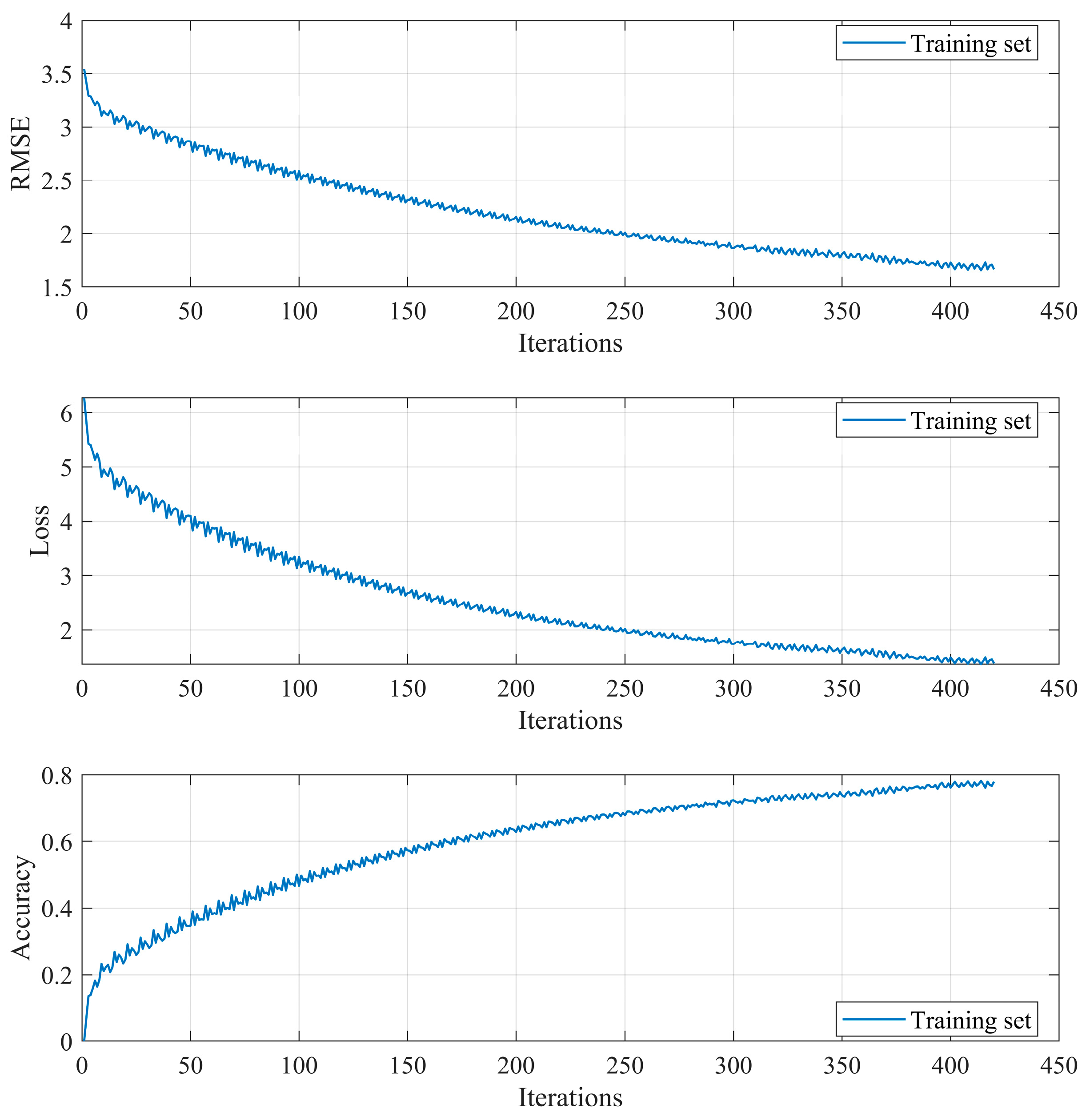
Figure 3 clearly illustrates the key dynamics of the model’s learning process, specifically the evolution of training performance in terms of RMSE, Loss, and Accuracy. The curves demonstrate a favorable convergence behavior throughout training.

3.4. Probabilistic Interval Prediction

Time series data typically exhibit a dynamic nature, uncertainty, and susceptibility to noise interference. The core advantage of probabilistic interval prediction over traditional point prediction lies in its ability to quantify uncertainty, enabling better adaptation to data fluctuations and interference, thereby providing a basis for decision-making.

In this study, a Gaussian-based probabilistic interval prediction method is employed, which leverages the normal distribution assumption and statistical characteristics of errors for calculation. According to the target confidence level, the uncertainty is estimated using the quantile function of the normal distribution and the prediction errors of the validation set, which is used to determine the width of the confidence interval. The calculation formulas for the upper and lower bounds of the confidence interval are as follows:

$${\widehat{y}}_i^u(\alpha )={\widehat{y}}_i+Z(\alpha )\cdot {\sigma }_e\cdot \sqrt{1+{\displaystyle \frac{1}{N_{valid}}}}$$

(11)

$${\widehat{y}}_i^l(\alpha )={\widehat{y}}_i-Z(\alpha )\cdot {\sigma }_e\cdot \sqrt{1+{\displaystyle \frac{1}{N_{valid}}}}$$

(12)

where ${\widehat{y}}_i$ is the point prediction value of the i-th sample, $Z(\alpha )$ is the quantile corresponding to the confidence level $\alpha$, ${\sigma }_e$ is the standard deviation of the validation set error, $N_{valid}$ is the sample size of the validation set.

As the sample size decreases, the interval becomes wider to address uncertainty. By dynamically adjusting the interval width, the probabilistic interval better aligns with the actual characteristics of the data.

4. Results Analysis

4.1. Relief Feature Selection

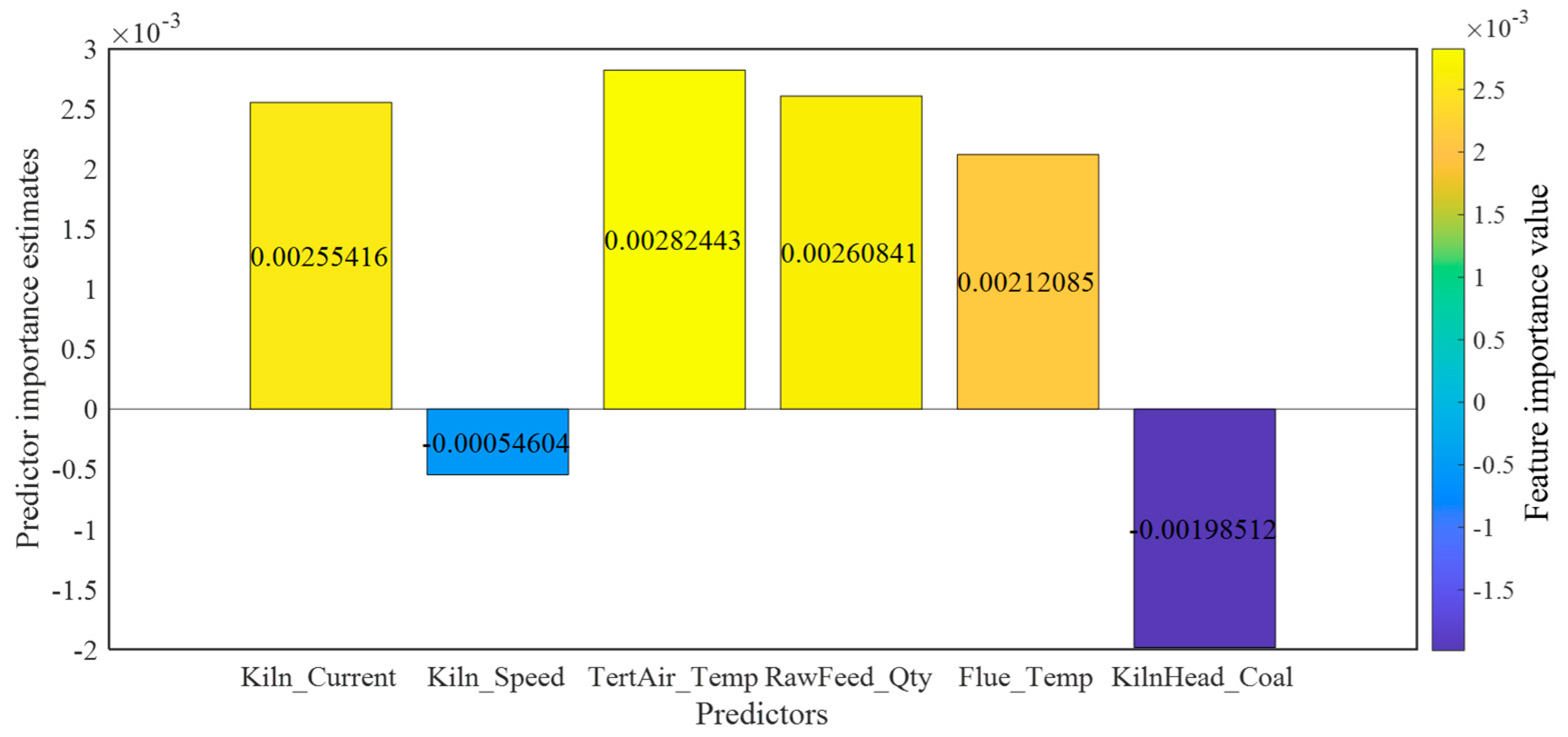
As shown in Figure 4, the Relief algorithm ultimately screened three core features: tertiary air temperature (TertAir_Temp), raw meal feed rate (RawFeed_Qty), and rotary kiln current (Kiln_Current). This result is highly consistent with the thermal balance mechanism of the rotary kiln calcination process, and the role and importance of each feature are analyzed as follows:

Tertiary air temperature (TertAir_Temp): As a key parameter of the combustion-supporting air in the kiln, it directly affects fuel combustion efficiency. Its fluctuations are transmitted to the kiln head temperature, making it a core characteristic variable of the heat input process. It has the highest importance because its fluctuation pattern in the dataset exhibits the strongest instantaneous correlation with the kiln head temperature, stably reflecting changes in heat input.

Raw meal feed rate (RawFeed_Qty): As an input parameter of the heat-absorbing carrier, it is directly related to heat consumption and serves as a core operational variable for thermal balance adjustment. It ranks second in importance: as a manually regulated slow variable, its lagged correlation with temperature is stable in time series data. However, due to its low adjustment frequency, its contribution is slightly lower than that of tertiary air temperature.

Rotary kiln current (Kiln_Current): It indirectly reflects the material filling rate and movement state inside the kiln. An abnormal increase in current often indicates risks of ring formation or material blockage, which affects the kiln head temperature by changing the flame shape, making it an important early warning indicator for operational stability. Its slightly lower importance is due to its nonlinear impact on temperature, but it is irreplaceable in capturing non-thermal interference factors.

These three features together form a characteristic system covering heat input, heat consumption, and operational stability, encompassing several key dimensions that influence the kiln head temperature.

4.2. Model Performance Analysis

4.2.1. Fitting Performance

Figure 5a presents the density plot of the training set, which exhibits an excellent fitting performance. The dense color area is concentrated around the fitting line, indicating that the model has learned sufficiently from the training set and can capture the inherent patterns of the data. Figure 5b shows the density plot of the validation set, where the data density is slightly lower than that of the training set. In contrast, the fitting performance of the test set (Figure 5c) is slightly inferior to that of the training and validation sets, but it still maintains a high standard, demonstrating the model’s strong overall generalization ability.

Figure 6 displays the joint density plot of the training set and test set. The true values of the training set cluster around the training fitting line, showing a narrow-band distribution along the line, which reflects the model’s high prediction accuracy. Additionally, the bandwidth of the 95% confidence interval for the training set is relatively narrow, indicating lower prediction uncertainty of the model for the training data. In contrast, the fitting deviation of the test set is larger than that of the training set, and the bandwidth of the 95% confidence interval for the test set is wider, resulting in higher prediction uncertainty for the test data. This is because the test data are new and not involved in model training, making error fluctuations more difficult to predict; thus, a wider interval is required to cover the true values. Overall, the model still maintains good fitting performance and strong generalization ability.

4.2.2. Prediction Capability

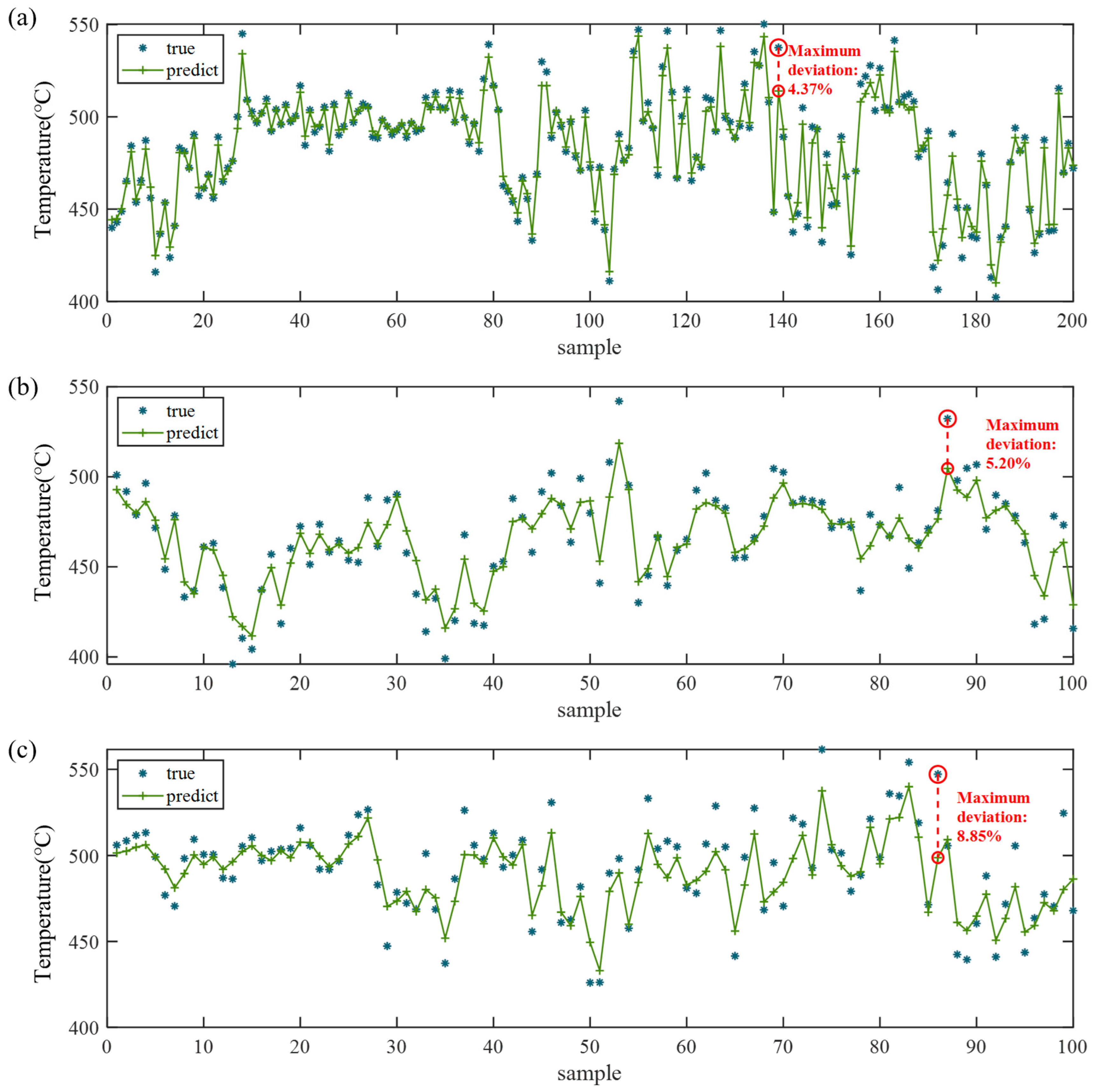
Figure 7 illustrates the comparison curves between the predicted results of the optimized CNN-BiLSTM-RF model and the true values for partial data in the training set, validation set, and test set, respectively.

Specifically, in Figure 7a (training set), the green predicted curve is consistent with the overall trend of the blue true value scatter points. Even in high-frequency fluctuation intervals, the predicted curve can oscillate and rise or fall accurately following the true values, exhibiting almost no significant lag or deviation. This indicates that the model has fully learned the fluctuation patterns of the time series data on the training set.

In Figure 7b (validation set), the predicted curve still captures the overall trend of the true values, demonstrating that the model has partially transferred the patterns learned from the training process to the validation data.

In contrast, Figure 7c (test set) shows that the predicted curve can roughly follow the core trend of the true values, which verifies the generalizability of the core time series patterns learned by the model. However, local deviations increase slightly, which reflects the novelty of the test data (not involved in training) and may also be attributed to data distribution differences or noise that enhance prediction uncertainty. Nevertheless, the model’s predicted values still track the variation trend of the true values well, and maintain high prediction accuracy even in regions with large temperature fluctuations—confirming the model’s strong adaptability and generalizability.

4.2.3. Model Performance Comparison

The performance of the optimized CNN-BiLSTM-RF model was compared with that of three single models (CNN, BiLSTM, and RF). The performance comparison results of all models on the test set are presented in

Table 1. Performance of Various Models on the Test Set.

Model	MAE	MAPE	MSE	RMSE	R2	Average Time
CNN	12.843	0.027454	274.09	16.556	0.75727	330.69
BiLSTM	9.889	0.02115	157.19	12.537	0.8608	266.9
RF	11.589	0.024794	252.51	15.891	0.77638	45.95
Opt-CNN-BiLSTM-RF	9.2792	0.019929	142.97	11.957	0.87482	1178.2

.

As shown in Table 1, the optimized CNN-BiLSTM-RF model outperforms the other comparative models in all evaluation metrics. Compared with the single CNN, BiLSTM, and RF models, the optimized model achieves a 27.7% reduction in Mean Absolute Error (MAE), a 27.4% reduction in Mean Absolute Percentage Error (MAPE), a 47.8% reduction in Mean Squared Error (MSE), a 27.8% reduction in Root Mean Squared Error (RMSE), and a 15.5% increase in coefficient of determination (R²). These results indicate that the optimized CNN-BiLSTM-RF model can effectively improve prediction performance and has obvious advantages in capturing complex dependencies and dynamic features among multiple variables, thus verifying the effectiveness of the heterogeneous ensemble.

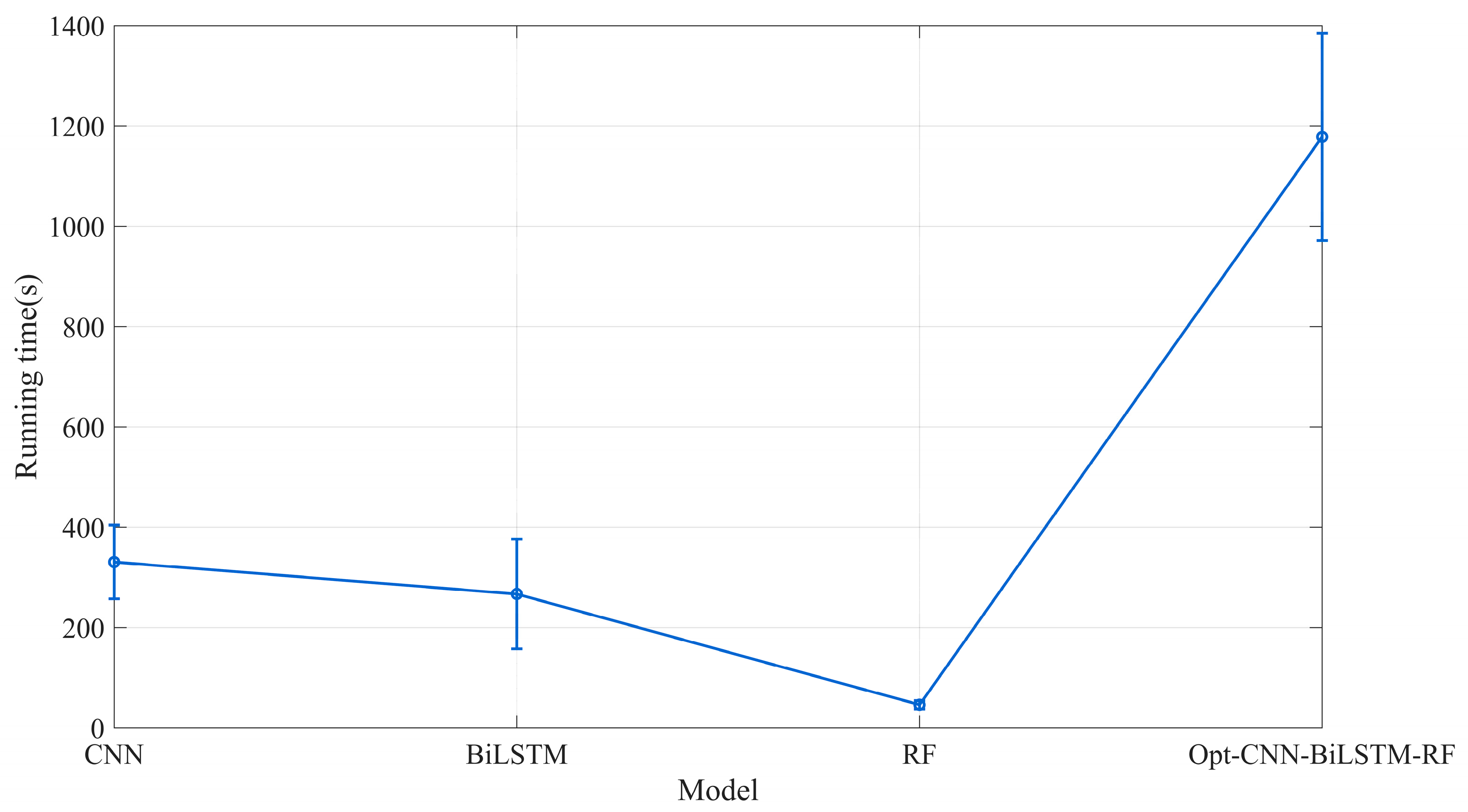
Figure 8 presents a comparison of the average runtime across the four models. The results indicate that the enhanced performance of the hybrid model is accompanied by a notably higher computational overhead. Therefore, model selection requires a deliberate consideration of the trade-off between predictive capability and running efficiency.

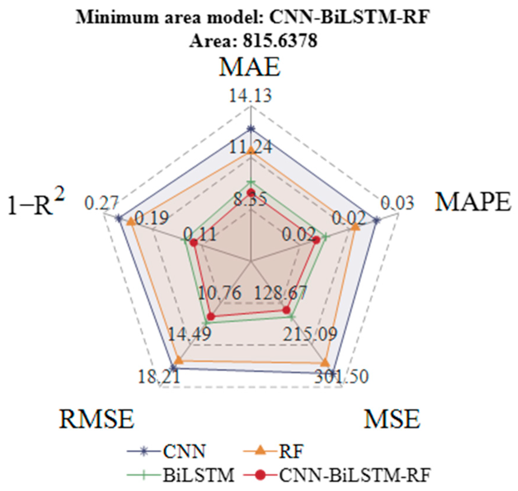
To more intuitively reflect the performance differences between models, the evaluation metrics were visualized using a radar chart, as shown in Figure 9.

Figure 9 compares the performance of CNN, BiLSTM, RF, and the optimized CNN-BiLSTM-RF across five core model metrics (MAE, MAPE, MSE, RMSE, and 1 − R²), where smaller values indicate better performance for all metrics. It can be easily observed from the chart that the performance of each model can be judged by the area enclosed by its metric values. Among all models, the optimized CNN-BiLSTM-RF encloses the smallest area and outperforms the single models in all metrics, confirming its optimal performance. This verifies the effectiveness of the proposed model in time series prediction tasks, as it balances both prediction accuracy and generalizability.

4.3. Probabilistic Interval Time Series Prediction

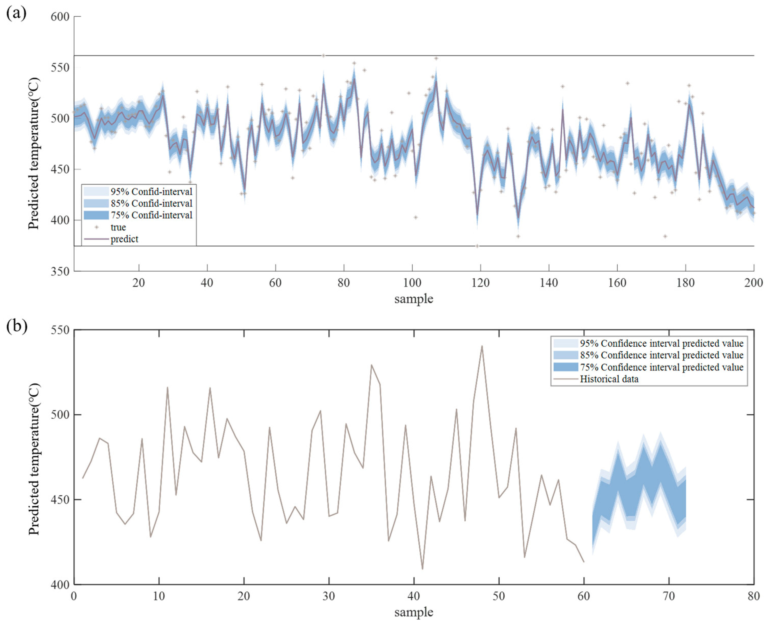
Figure 10a presents the multi-confidence level time series prediction fitting comparison chart, which includes three confidence intervals (75%, 85%, and 95%) distinguished by filled bands ranging from light blue to dark blue. Consistent with statistical principles, the higher the confidence level, the wider the interval bandwidth. Notably, most true values fall within each confidence interval, indicating that the uncertainty estimation of the model is reasonable. Additionally, the fitted curve of predicted values aligns well with the overall distribution trend of true values and can even capture local small-scale fluctuations—fully demonstrating the model’s high prediction accuracy for training data points.

Figure 10b shows the future trend prediction confidence interval chart. The initial shape of the future prediction interval connects naturally with the tail trend of historical data, the fluctuation characteristics of historical data near the 60th sample point are inherited by the initial shape of the prediction interval, which proves that the model considers the continuity of historical trends during extrapolation.

Furthermore, the bandwidth of the future interval does not expand excessively as the prediction step increases, and the oscillation pattern inside the interval is similar to the actual fluctuation characteristics of historical data. This reflects the model’s ability to reasonably quantify future uncertainty: it not only inherits historical patterns but also covers potential risks through the designed intervals, providing reliable decision support for future operational adjustments of the rotary kiln.

The probabilistic interval forecasts generated in this study can be directly applied to quantify risks in industrial control decisions. For instance, in a kiln temperature control scenario, the predictions with a 95% confidence interval quantify the risk range of “actual temperature deviating from the predicted value.” If the prediction interval encompasses the process-allowed temperature threshold, the associated decision risk is low, and current control parameters can be maintained. Conversely, if the interval exceeds the threshold, control strategies must be adjusted based on the interval’s characteristics—such as increasing the monitoring frequency when the interval is too wide, or preemptively raising the temperature when the lower bound falls below the threshold. This approach provides a quantifiable basis for enhancing the robustness of industrial control systems.

4.4. Discussion

Feature Selection: The Relief algorithm was employed to identify and retain core features strongly correlated with the prediction target, thereby eliminating redundant information and reducing model computational complexity as well as the risk of overfitting.

Data Preprocessing: Variational Mode Decomposition (VMD) was applied to effectively separate the target signal from noise, enhancing data quality and providing cleaner temporal features for model learning.

Model Architecture: The CNN component extracts local spatial correlations within the temporal data through convolutional operations, capturing underlying relationships between features at adjacent time steps while mitigating interference from irrelevant information.

The BiLSTM layer utilizes both forward and backward LSTM units to simultaneously capture past and future dependencies in the time series data, adapting to the dynamic characteristics of industrial processes.

The RF model, based on ensemble learning with multiple decision trees, enhances the model’s capacity to fit nonlinear relationships, reduces overfitting risks associated with single models, and provides robust decision support for the fused framework.

Fusion Strategy: An adaptive weighting mechanism, based on the Mean Absolute Error (MAE) on the validation set, dynamically allocates weights to the two model branches. This approach leverages the strengths of each individual model while compensating for its respective limitations, thereby achieving overall performance improvement.

5. Conclusions

To address the kiln head temperature prediction problem of rotary kilns, this study proposes an optimized CNN-BiLSTM-RF time series prediction framework based on Relief feature selection and adaptive weight integration. Through preprocessing of industrial data and feature engineering, rich dynamic features are extracted; by introducing an adaptive weight mechanism, the proposed model effectively enhances the ability to capture key variables and long-distance dependencies. Experimental results show that this method outperforms traditional machine learning models and existing deep learning models in prediction accuracy, providing effective technical support for the stable operation of rotary kilns. Specific conclusions are as follows:

(1) Data preprocessing and feature selection ensure data validity and feature specificity, laying a solid foundation for subsequent model training.

(2) The proposed fusion strategy integrates the advantages of CNN, BiLSTM, and RF: CNN captures spatial coupling features, BiLSTM models bidirectional temporal dependencies, and RF enhances robustness—collectively significantly improving prediction accuracy.

(3) The introduction of an adaptive weight mechanism enables the model to dynamically adjust the contribution of each sub-model according to data characteristics, thereby enhancing its adaptability to dynamic industrial data.

(4) Gaussian probabilistic intervals are utilized to achieve reasonable quantification of prediction uncertainty, which not only quantifies potential risks but also supports reliable prediction of future temperature trends.

(5) The error variation from the training set to the test set and the comparison of multiple evaluation metrics verify that the model balances both fitting accuracy and generalization ability, meeting the requirements of practical industrial applications.

Limitations of This Study:

The limited dataset size may lead to insufficient learning of temporal features under extreme operating conditions, and the model’s generalization capability requires further validation.

Dependence on Hyperparameters: Key hyperparameters, such as the number of IMFs in VMD and the size of CNN convolutional kernels, require manual adjustment based on empirical experience. The current framework lacks an adaptive optimization mechanism for these parameters.

Simplistic Fusion Strategy: The fusion weights are assigned solely based on the Mean Absolute Error (MAE) metric. This approach does not incorporate other statistical characteristics of the predictions, such as variance or skewness, which could provide a more comprehensive basis for fusion.

Future Research Directions:

Automatic Hyperparameter Tuning: Future work will explore the integration of advanced optimization techniques, including Bayesian optimization and genetic algorithms, to automate the hyperparameter search process. This aims to enhance model performance while reducing reliance on manual intervention.

Multi-Metric Fusion Strategy: Subsequent research will focus on developing a more sophisticated fusion strategy. This involves constructing a weighted matrix that incorporates multiple metrics—such as variance and Mean Absolute Percentage Error (MAPE)—to more effectively leverage the strengths of each constituent model and improve overall predictive robustness.

Incorporate interpretability techniques such as SHAP or Grad-CAM to visualize the decision-making process of the CNN-BiLSTM-RF model and quantify the contribution of key features to the predictions.

Expand the current single-target prediction to multi-target forecasting, thereby providing more comprehensive decision support for industrial control.