A Hybrid EMD–LASSO–MCQRNN–KDE Framework for Probabilistic Electric Load Forecasting Under Renewable Integration

Abstract

Accurate probabilistic load forecasting is essential for secure power system operation and efficient energy management, particularly under increasing renewable integration and demand-side complexity. However, traditional forecasting methods often struggle with issues such as non-linearity, non-stationarity, feature redundancy, and quantile crossing, which hinder reliable uncertainty quantification. To overcome these challenges, this study proposes a hybrid probabilistic load forecasting framework that integrates empirical mode decomposition (EMD), LASSO-based feature selection, and a monotone composite quantile regression neural network (MCQRNN) enhanced with kernel density estimation (KDE). First, EMD decomposes the raw load series into intrinsic mode functions and a trend component to mitigate non-stationarity. Then, LASSO selects the most informative features from both the decomposed components and the original time series, effectively reducing dimensionality and multicollinearity. Subsequently, the proposed MCQRNN model generates multiple quantiles under monotonicity constraints, eliminating quantile crossing and improving multi-quantile coherence through a composite loss function. Finally, Gaussian kernel density estimation reconstructs a continuous probability density function from the predicted quantiles, enabling full distributional forecasting. The framework is evaluated on two public datasets—GEFCom2014 and ISO New England—using point, interval, and density evaluation metrics. Experimental results demonstrate that the proposed EMD–LASSO–MCQRNN–KDE model outperforms benchmark approaches in both point and probabilistic forecasting, providing a robust and interpretable solution for uncertainty-aware grid operation and energy planning.

1. Introduction

With the acceleration of global energy transition and the evolution of power systems toward high-penetration renewable energy and power-electronics-dominated infrastructure, accurate load forecasting and effective uncertainty quantification have become central to ensuring grid stability and optimizing resource allocation [1]. On one hand, the strong volatility of renewable generation—such as wind and solar—requires precise load forecasts to maintain supply-demand balance. According to the International Energy Agency (IEA), renewable sources accounted for 28% of global electricity generation in 2023, and every 1% increase in load forecasting error can raise grid reserve costs by 0.5–1.2% [2]. On the other hand, diversified consumer behaviors—including electric vehicle charging and industrial flexible loads—introduce heightened non-linearity and randomness into load patterns. Traditional point forecasting models, such as ARIMA, are increasingly inadequate for capturing risk probabilities required by modern dispatch decisions [3]. Consequently, research focus has shifted from deterministic point predictions to probabilistic distribution forecasting, enabling comprehensive uncertainty quantification for grid scheduling, energy storage planning, and pricing strategies [4]. This paradigm shift has positioned probabilistic load forecasting as a critical research frontier in energy systems [5].

Electric load time series exhibit pronounced non-linearity and non-stationarity due to influences from weather, social activities, and seasonal cycles, posing significant challenges to conventional forecasting models [6,7,8]. For instance, air conditioning surges during heatwaves or distinct weekday-weekend consumption patterns lead to complex multi-scale dynamics: short-term (hourly) fluctuations are often masked by noise, mid-term (daily) cycles show peak-valley regularity, and long-term (seasonal) trends reflect structural shifts [9]. To address this, data decomposition techniques have been widely adopted to break down complex load signals into simpler components. Empirical Mode Decomposition (EMD), an adaptive method that extracts physically meaningful intrinsic mode functions (IMFs) without predefined basis functions, has proven effective in preprocessing non-stationary load data [10]. For example, EMD-based decomposition has reduced prediction errors by 15–20% in certain studies by separating high-frequency noise, daily cycles, and seasonal trends [11]. However, most existing approaches couple EMD with single forecasting models, neglecting potential redundancy among decomposed components, which may lead to overfitting and increased model complexity [12]. Thus, a synergistic preprocessing strategy combining EMD with feature selection—termed “EMD + feature selection’’—remains underexplored and warrants further investigation [13].

The quality of input features critically determines model performance in load forecasting. Redundant features—such as high-frequency noise components or weakly correlated lagged variables—can increase computational burden and induce multicollinearity, while missing key predictors may result in underfitting [14]. Feature selection thus serves as a vital bridge between data preprocessing and predictive modeling. The Least Absolute Shrinkage and Selection Operator (LASSO), which employs L1 regularization to shrink irrelevant coefficients to zero, enables simultaneous parameter estimation and variable selection, offering both simplicity and interpretability [15]. Similarly, LASSO has been used to eliminate redundant high-frequency IMFs after EMD, enhancing the generalization of SVR models [16]. Nevertheless, most current research integrates LASSO with traditional machine learning models, and joint selection of EMD-derived components and historical load features remains rare [17]. Moreover, in-depth analysis of the relationship between selected features and load distribution is often lacking, limiting the full potential of feature selection in supporting probabilistic forecasting [18].

To quantify uncertainty in load forecasting, quantile regression (QR) has emerged as a core technique. By estimating conditional quantiles at different confidence levels, QR provides prediction intervals without assuming a specific error distribution (e.g., normality) [19]. However, traditional linear QR struggles to capture the non-linear dynamics of load data. This limitation has driven the development of Quantile Regression Neural Networks (QRNN), which leverage the non-linear modeling capacity of neural networks to enhance QR’s applicability [20]. QRNN has shown promise in probabilistic load forecasting; for example, one study achieved a 92% prediction interval coverage probability (PICP) at a 90% confidence level [21]. Other works have improved QRNN by refining loss functions to better capture extreme load events [22]. Despite these advances, QRNN suffers from the “quantile crossing” problem—where higher quantiles are predicted below lower ones—leading to logically inconsistent intervals [23]. Additionally, most QRNN models optimize individual quantiles independently, lacking joint constraints across multiple quantiles, which compromises the overall coherence of the predicted distribution [24]. Therefore, integrating monotonic quantile constraints with composite quantile loss functions represents a key direction for developing more robust and logically consistent probabilistic models [25].

While quantile regression provides discrete quantile estimates, it does not yield a continuous probability density function (PDF). A continuous PDF, however, offers a more intuitive representation of load likelihood across different values, which is crucial for risk assessment—such as evaluating the probability of extreme peak loads [26]. Kernel Density Estimation (KDE), a nonparametric method, reconstructs smooth density curves from discrete samples without assuming a specific distribution form, thereby bridging the gap between quantile forecasts and full density estimation [27]. In load forecasting, KDE has been applied to transform quantile outputs into continuous PDFs; for instance, combining QRNN with KDE enabled the quantification of wind integration impacts on load distribution. Similarly, KDE has been integrated with LSTM-based quantile forecasts to generate probabilistic load densities in distribution networks. However, most existing studies rely on conventional QRNN outputs, failing to account for the adverse effects of quantile crossing on density reconstruction. Furthermore, KDE bandwidths are often set empirically, lacking adaptive optimization tailored to load characteristics, which may result in oversmoothing or loss of detail [28]. Hence, a unified probabilistic forecasting framework that combines non-crossing quantile prediction with adaptive KDE remains to be fully developed.

To address the limitations in current research—insufficient handling of non-linearity, ineffective removal of feature redundancy, quantile crossing, and suboptimal density reconstruction—this study proposes a novel probabilistic load forecasting framework based on Monotone Composite Quantile Regression Neural Network (MCQRNN) and Gaussian kernel density estimation. The primary objectives are threefold: (1) to implement an EMD-LASSO hybrid preprocessing strategy for multi-scale decomposition and key feature selection, reducing modeling complexity; (2) to develop an MCQRNN model that enforces monotonicity constraints to eliminate quantile crossing and employs composite quantile loss to improve multi-quantile fitting accuracy; and (3) to reconstruct continuous load probability density functions using KDE based on MCQRNN outputs, achieving a full-chain uncertainty quantification from point to interval to density forecasting. The proposed method is evaluated on two benchmark datasets—GEFCom2014 and ISO New England (ISO-NE)—across three dimensions: point prediction accuracy, quantile validity, and density reliability. This work aims to provide more robust forecasting support for power system operations while advancing the methodological framework for probabilistic forecasting of non-stationary time series.

To be specific, targeting the issues of non-linearity, non-stationarity, feature redundancy, and quantile crossing existing in electric load forecasting under renewable energy grid integration, this study aims to propose a hybrid probabilistic forecasting framework to achieve accurate electric load prediction. Based on two public datasets, namely GEFCom2014 and ISO New England, this paper first decomposes the original load sequence into IMFs and a trend component via EMD to reduce non-stationarity. Subsequently, LASSO is adopted to select key features for mitigating redundancy and multicollinearity. Then, a monotonic composite quantile regression neural network (MCQRNN) with monotonicity constraints is utilized to generate non-crossing multi-quantile prediction results. Finally, kernel density estimation (KDE) is employed to reconstruct the discrete quantiles, thereby realizing probabilistic forecasting.

2. Proposed Methods

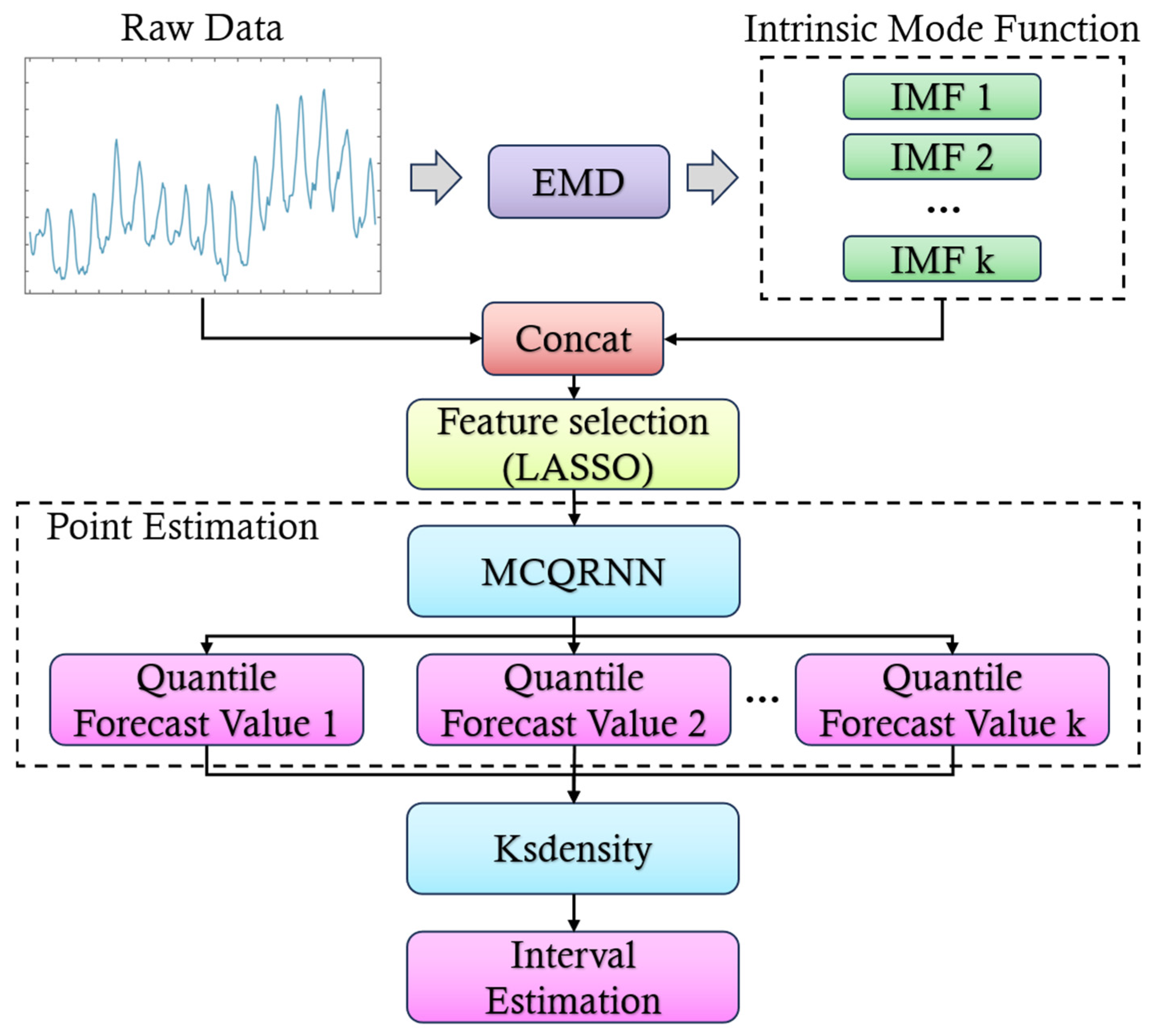
As illustrated in Figure 1, the raw electric load data often exhibits characteristics of non-linearity and non-stationarity. To address these challenges, EMD technique is employed to decompose the original time series of electric load data into multiple IMFs. This process extracts components with varying frequencies and fluctuation features from the raw data, ranging from high-frequency random fluctuations to low-frequency trend variations. The original electric load data are then concatenated with the obtained IMFs.

Following this, feature selection is performed using the LASSO method. This step identifies the most influential features for electric load forecasting while eliminating redundant information and reducing data dimensions. Subsequently, a MCQRNN is utilized for point estimation, generating a series of quantile predictions that comprehensively characterize the uncertainty distribution in electric load forecasting outcomes.

Finally, based on these quantile predictions, kernel density estimation (KDE) is applied to estimate the probability density distribution of the forecasts. This facilitates interval estimation, providing a robust framework for understanding the variability and uncertainty inherent in electric load predictions.

2.1. Empirical Mode Decomposition

EMD is a versatile method for the analysis of non-linear and non-stationary signals [29]. It aims to decompose the original signal into several IMFs along with a residual term that captures the overall trend [30]. Two key considerations underpin the selection of EMD over other decomposition techniques such as VMD and CEEMDAN in this study:

First, electric load data inherently exhibits strong periodicity. EMD does not require prior parameters (e.g., preset number of decomposition modes or basis functions) and can adaptively extract IMFs based on the time-scale characteristics of the electric load sequence itself. In contrast, VMD demands predefinition of the number of modes—improper parameter selection may lead to over-decomposition or under-decomposition. While CEEMDAN can suppress mode mixing, it still relies on noise parameter settings, resulting in weaker adaptability than EMD.

Second, in terms of computational efficiency, EMD’s decomposition process does not involve complex iterative optimization. Compared with other methods such as VMD (which uses the alternating direction method of multipliers) and CEEMDAN (which requires multiple noise additions and ensemble averaging), EMD significantly reduces computational time consumption.

The decomposition process, known as sifting, follows these steps:

Given an initial signal $x\left(t\right)$, set the first residue $r_0\left(t\right)=x\left(t\right)$ and initialize the IMF index $i$ to 1. To extract the $i$-th IMF, use the current residue $r_{i-1}\left(t\right)$ as input, denoted as $h\left(t\right)$ [31]. In each iteration, identify all local maxima and minima of $h\left(t\right)$, fit upper and lower envelopes using cubic spline interpolation ($e_{\max }\left(t\right)$ and $e_{\min }\left(t\right)$), and calculate their average:

$$m(t)={\displaystyle \frac{e_{\mathrm{m}\mathrm{a}\mathrm{x}}\left(t\right)+e_{\mathrm{m}\mathrm{i}\mathrm{n}}\left(t\right)}{2}},$$

(1)

Subtract this mean from $\mathrm{h}\left(\mathrm{t}\right)$ to obtain an updated version:

$$h\left(t\right)\leftarrow h\left(t\right)-m\left(t\right),$$

(2)

This iterative process continues until $h\left(t\right)$ meets the criteria for an IMF: the number of extrema and zero crossings must be equal or differ by one, and the local means of the envelopes should approach zero. Convergence is typically assessed using the standard deviation (SD):

$$\mathrm{S}\mathrm{D}={\displaystyle \frac{\sum _t {\left|h_{k-1}\left(t\right)-h_k\left(t\right)\right|}^2}{\sum _t h_{k-1}^2\left(t\right)}},$$

(3)

where convergence is achieved when SD falls below a specified threshold 0.3. At this point, $h\left(t\right)$ becomes ${IMF}_i\left(t\right)$, and the residue is updated:

$$r_i\left(t\right)=r_{i-1}\left(t\right)-{IMF}_i\left(t\right),$$

(4)

If $r_i\left(t\right)$ contains at least two extrema, it suggests further oscillatory components are present, prompting the continuation of the IMF extraction process; otherwise, the procedure ends, with $r_i\left(t\right)$ being the final residue.

The original signal $x\left(t\right)$ is thus represented as the sum of all IMFs and the final residue:

$$x(t)={\sum }_{i=1}^k {IMF}_i(t)+r(t),$$

(5)

where each ${IMF}_i\left(t\right)$ encapsulates different oscillatory patterns within the signal, ranging from high-frequency fluctuations to low-frequency trends, while $r\left(t\right)$ embodies the long-term trend.

2.2. Feature Selection Based on LASSO

After performing EMD, the original signal is decomposed into multiple Intrinsic Mode Function (IMF) components. These IMFs encapsulate information across various time scales. To enhance the performance and interpretability of predictive models, it is essential to select the most influential features from these IMF components for the prediction target. The LASSO is a linear regression technique that achieves both variable selection and parameter estimation by incorporating an L1 regularization term. Its fundamental form can be expressed as:

$$\underset{{\beta }^L}{\mathrm{m}\mathrm{i}\mathrm{n}} \left\{{\sum }_{t=1}^T {\left(y_t-{\sum }_{m=1}^M {\beta }_m^L{x}_{t,m}\right)}^2+v{\sum }_{m=1}^M \left|{\beta }_m^L\right|\right\},$$

(6)

Here, $\mathrm{T}$ represents the sample size, $y_t$ and $x_{t,m}$ denote the response variable and predictor variables for the $t$-th sample, respectively, while ${\beta }_m^L$ corresponds to the coefficient for the $\mathrm{m}$-th feature. The inclusion of the L1 penalty term $\nu {\sum }_{m=1}^M \left|{\beta }_m^L\right|$ allows for the coefficients of less impactful or irrelevant predictors to approach zero, thereby simplifying the model and mitigating over-fitting. The parameter $v$, a non-negative regularization constant, controls the degree of shrinkage; larger values of $\mathrm{v}$ impose stricter penalties, leading to fewer retained variables.

Assuming ${\widehat{\beta }}^L$ is the coefficient estimator in LASSO, it can be computed by minimizing the residual sum of squares subject to a linear constraint, as follows:

$$\begin{array}{rr}{\widehat{\beta }}^L& =\mathrm{a}\mathrm{r}\mathrm{g}\underset{\beta }{\mathrm{m}\mathrm{i}\mathrm{n}} \left\{{\sum }_{t=1}^T {\left(y_t-{\sum }_{m=1}^M {\beta }_m^L{x}_{t,m}\right)}^2\right\}\\ & \end{array},$$

(7)

$$\mathrm{s}.\mathrm{t}.{\sum }_{m=1}^M \left|{\beta }_m^L\right|\le \delta ,$$

(8)

The parameter $\delta$ is inversely related to $\mathrm{v}$. Optimal values for $\mathrm{v}$ can be determined through methods such as cross-validation (CV) or generalized cross-validation (GCV). After iterative optimization, certain variable coefficients in the LASSO regression may be reduced to zero. Variables with zero coefficients are deemed insignificant and are thus excluded from the model. This process ensures that only the most relevant features contribute to the final predictive model, enhancing its accuracy and interpretability.

2.3. Monotonic Composite Quantile Regression Neural Network (MCQRNN)

Following the feature selection using LASSO, this study employs a Monotonic Composite Quantile Regression Neural Network (MCQRNN) to achieve robust and high-resolution multi-quantile predictions for the target variable. This method integrates the statistical stability of composite quantile regression (CQR) with the non-linear modeling capabilities of neural networks. Additionally, it imposes structural constraints to ensure the monotonicity of predicted quantile sequences, thereby avoiding the issue of quantile crossing and enhancing the rationality and interpretability of the prediction results.

The MCQRNN model is defined as follows:

$$\begin{array}{ll}{Q}_{y_t}\left(\theta \mid x_t\right)=f\left(x_t,G\left(\theta \right),H\left(\theta \right)\right)=& l_2\left\{{\displaystyle \sum _{k=1}^K} l_1\left[{\displaystyle \sum _{i\in I}} x_i\mathrm{e}\mathrm{x}\mathrm{p}\left(g_{i,k}\left(\theta \right)\right)\right.\right.\\ & \left.\left.+{\displaystyle \sum _{l\in L}} x_l{g}_{l,k}\left(\theta \right)+b_{t,m}^h\right]\times \mathrm{e}\mathrm{x}\mathrm{p}\left(h_k\left(\theta \right)\right)+b_t^o\right\}\end{array}$$

(9)

Here, $\mathrm{I}$ denotes the index set corresponding to explanatory variables that exhibit a monotonically increasing relationship with the target electric load. In contrast, $L$ represents the index set for covariates in $x_t$ that do not impose such a monotonic constraint-meaning their association with the load lacks a fixed increasing or decreasing trend. $G\left(\theta \right)$ refers to the weight matrix (note: corrected from “vector” for consistency with layer connection logic) linking the input layer to the hidden layer, while $H\left(\theta \right)$ denotes the weight matrix connecting the hidden layer to the output layer; both sets of weights are adjusted dynamically with the quantile level $\theta$ to ensure the rationality of quantile predictions. $K$ indicates the number of hidden layer nodes (i.e., hidden layer size), a key hyperparameter tuned during model training. Meanwhile, $b^h$ and $b^o$ stand for the bias vectors of the hidden layer and output layer, respectively, which help the model fit complex load dynamics by offsetting linear mapping deviations. $l_1(\cdot )$ denotes the activation function of the hidden layer, with the hyperbolic tangent function as the common choice to introduce non-linearity into the model. $l_2(\cdot )$ represents the smooth non-decreasing inverse link function of the output layer, whose core role is to maintain the monotonicity of predicted quantiles (i.e., higher quantile levels correspond to larger predicted values) and avoid quantile crossing.

The optimal estimates of $\mathrm{G}(\mathsf{\theta })$ and $\mathrm{H}(\mathsf{\theta })$, denoted as $\stackrel{\mathrm{ˆ}}{\mathrm{G}}(\mathsf{\theta })$ and $\stackrel{\mathrm{ˆ}}{\mathrm{H}}(\mathsf{\theta })$, can be obtained by solving the following equation, thus yielding the conditional quantiles of $y_t$:

$$U(G(\theta ),H(\theta ))=\mathrm{m}\mathrm{i}\mathrm{n}{E}_{\theta }=\mathrm{m}\mathrm{i}\mathrm{n}{\displaystyle \frac{1}{T}}\sum _{l=1}^T {\zeta }_{\theta }\left(y_t-f\left(x_t,G\left(\theta \right),H\left(\theta \right)\right)\right)$$

(10)

Typically, parameters in the MQRNN model can be trained or estimated using gradient based non-linear optimization algorithms. However, the check function ${\zeta }_{\theta }\left(\sigma \right)$ is not always differentiable due to its undefined derivative at the origin. Therefore, we use the Huber norm, which provides a smooth approximation between absolute error and squared error near the origin, to replace the exact quantile regression loss function’s $\zeta \left(\sigma \right)$. The approximation is given by:

$${\bar{\zeta }}_{\theta }(\sigma )=\left\{\begin{array}{l}\theta \cdot \zeta \left(\sigma \right)\\ (\theta -1)\cdot \zeta \left(\sigma \right)\end{array}\right.$$

(11)

where $\zeta \left(\sigma \right)$ is the Huber function, ensuring a stable transition between absolute and squared errors:

$$\zeta (\sigma )=\left\{\begin{array}{ll}{\displaystyle \frac{{\sigma }^2}{2\varrho }}& 0\le \left|\sigma \right|\le \varrho \\ |\sigma |-{\displaystyle \frac{\varrho }{2}}& \left|\sigma \right|>e\end{array}\right.$$

(12)

Here, $\varrho$ represents the specified threshold value. Utilizing this approximate check function to update the MQRNN loss yields the empirical approximate loss function in Equation (10):

$$E_{\theta }={\displaystyle \frac{1}{T}}\sum _{t=1}^T {\tilde{\varphi }}_{\theta }\left(y_t-f\left(x_t,G\left(\theta \right),H\left(\theta \right)\right)\right)$$

(13)

However, the MQRNN model is unable to effectively prevent the crossing of multiple $\theta$ estimates. To address this issue, the MCQRNN model integrates the structural framework of the MQRNN with the error function of the CQRNN. The optimal estimates are obtained by optimizing the following approximate loss function:

$$E_{\theta }={\displaystyle \frac{1}{ZT}}\sum _{z=1}^Z \sum _{t=1}^T {\tilde{\zeta }}_{{\theta }_z}\left(y_t-f\left(x_t,G\left({\theta }_z\right),H\left({\theta }_z\right)\right)\right)$$

(14)

Here, ${\theta }_z={\displaystyle \frac{z}{z+1}}$, where $\mathrm{z}$ represents the size of the quantile.

By combining these elements, the MCQRNN model aims to enhance prediction accuracy while maintaining the integrity of the quantile relationships. This approach ensures that the estimated values remain consistent across different quantiles, thereby improving the overall reliability and interpretability of the model.

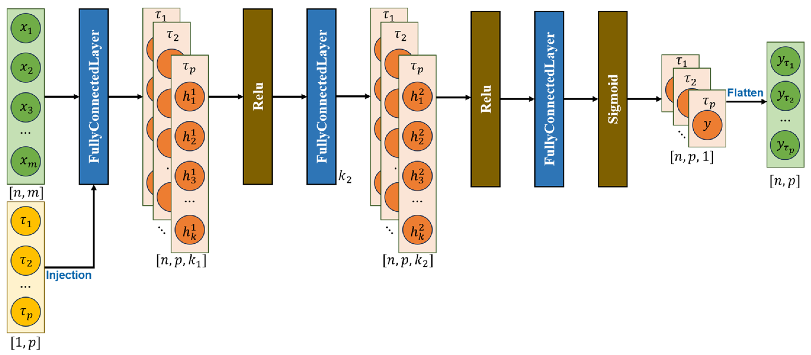
The specific network architecture of the model is illustrated in Figure 2. The experimental hyperparameter configuration is as follows: the number of training epochs is set to 10,000, and the learning rate is 0.05; the network architecture comprises two fully connected hidden layers, each with a dimension of 10; the ReLU activation function is adopted for the hidden layers, while the Sigmoid activation function is used for the output layer; the Adam optimizer is employed as the optimization algorithm.

2.4. Kernel Density Estimation

To further reconstruct the conditional probability density function from discrete quantile predictions and generate smooth probabilistic prediction intervals, this study introduces kernel density estimation (KDE) based on MCQRNN outputs. By leveraging the similarity between conditional quantiles and conditional densities, we use the obtained conditional quantiles $G_{t,z}$ as inputs to the KDE function to construct the probability density curve.

The conditional quantile predictions $G_{t,z}$ are treated as a set of independently and identically distributed samples. Their probability density estimates can be obtained using KDE:

$${\widehat{f}}_z(G)={\displaystyle \frac{1}{Zs}}\sum _{z=1}^Z C\left({\displaystyle \frac{G_{t,z}-G}{s}}\right)$$

(15)

Here, $Z$ represents the number of quantiles, $s$ denotes the bandwidth, and $C(\cdot )$ is a non-negative kernel function.

2.5. Evaluation Metrics

To further evaluate the performance of the model, in addition to using the Mean Absolute Percentage Error (MAPE), Root Mean Square Error (RMSE), and Mean Absolute Error (MAE) for quantifying the point prediction accuracy, we also incorporate the coefficient of determination ($R^2$), a measure of goodness-of-fit. Smaller values of MAPE, RMSE, and MAE indicate better deterministic predictive performance, while a higher $R^2$ value signifies a better fit between the predicted and actual values.

The expressions for these metrics are as follows:

$$MAPE={\displaystyle \frac{1}{T}}\sum _{t=1}^T \left|{\displaystyle \frac{R_t-{\widehat{R}}_t}{R_t}}\right|$$

(16)

$$RMSE=\sqrt{{\displaystyle \frac{1}{T}}\sum _{t=1}^T {\left(R_t-{\widehat{R}}_t\right)}^2}$$

(17)

$$MAE={\displaystyle \frac{1}{T}}\sum _{t=1}^T \left|R_t-{\widehat{R}}_t\right|$$

(18)

The coefficient of determination, $R^2$, is defined as:

$$R^2=1-{\displaystyle \frac{{\sum }_{t=1}^T {\left(R_t-{\widehat{R}}_t\right)}^2}{{\sum }_{t=1}^T {\left(R_t-\bar{R}\right)}^2}}$$

(19)

where $\bar{R}$ represents the mean of the actual values $R_t$. A higher $R^2$ value indicates that a greater proportion of the variance in the data is explained by the model, suggesting a better fit.

By incorporating these evaluation metrics, we can comprehensively assess the predictive performance and goodness-of-fit of the model, ensuring its reliability and effectiveness in practical applications.

3. Experimental Results Analysis

3.1. Dataset Description

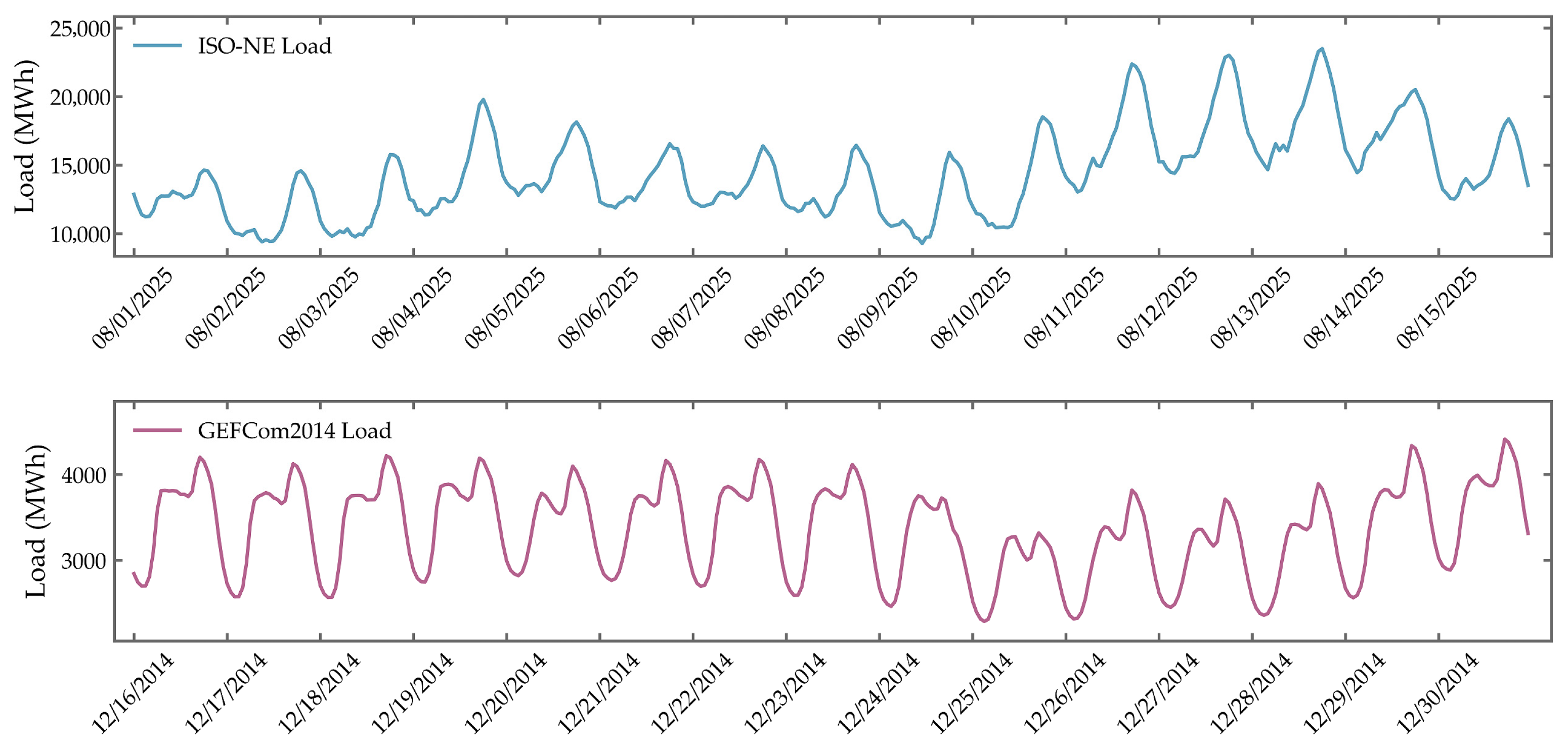
To validate the effectiveness and generalization capability of the MCQRNN model, historical electric load data from two widely recognized benchmark datasets are employed for comprehensive case studies: the Global Energy Forecasting Competition 2014 (GEFCom2014) and the ISO New England (ISO-NE) system load data. Figure 3 illustrates the time series characteristics of the load data in both datasets. In all cases, the datasets are partitioned into training and testing subsets following the same protocols as in existing studies to ensure a fair and reproducible comparison, particularly given that many deep learning-based load forecasting models lack publicly available code, making direct replication challenging. For the GEFCom2014 dataset, which contains hourly load records from 16 December 2004 to 30 December 2008, the period from 16 December 2004 to 29 December 2008 (noon) is used for training, while the remaining 36 hourly samples (from 29 December 2008, noon, to 30 December 2008) constitute the test set. Similarly, for the ISO-NE dataset (https://www.iso-ne.com/isoexpress/web/reports/load-and-demand, accessed on 20 November 2025), which includes hourly load data from 1 August 2025, to 15 August 2025, the interval from 1 August 2025, to 14 August 2025 (noon) is designated as the training subset, and the subsequent 36 hourly samples (from 14 August 2025, noon, to 15 August 2025) are reserved for testing. The proposed MCQRNN model is applied to generate probabilistic load forecasts over a 36 h horizon for both datasets, enabling a rigorous evaluation of its predictive accuracy, uncertainty quantification, and adaptability across different geographic and temporal contexts. This experimental setup ensures a robust assessment of the model’s performance under consistent evaluation criteria, facilitating reliable comparison with state-of-the-art methods.

3.2. Data Preprocessing and EMD Performance

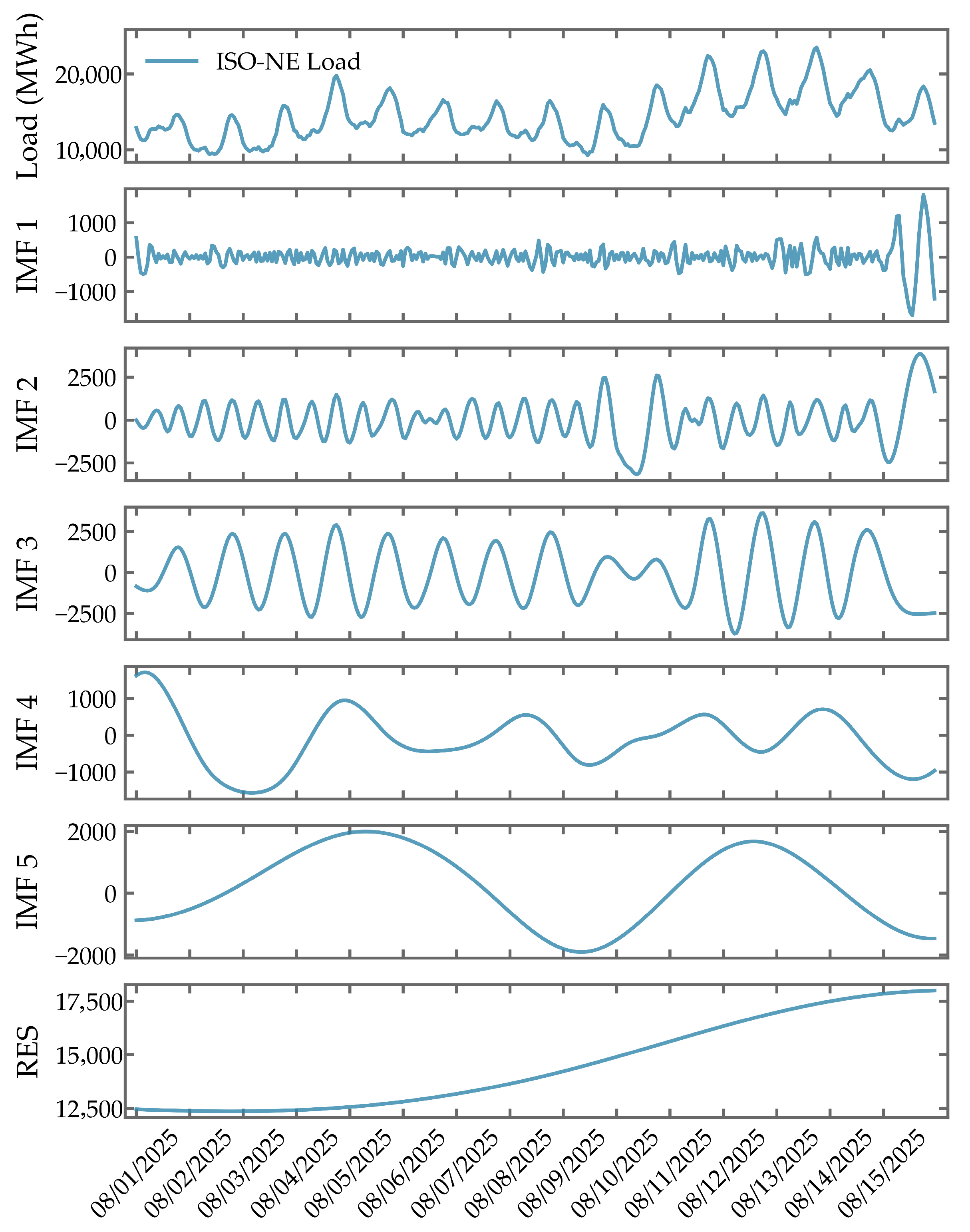
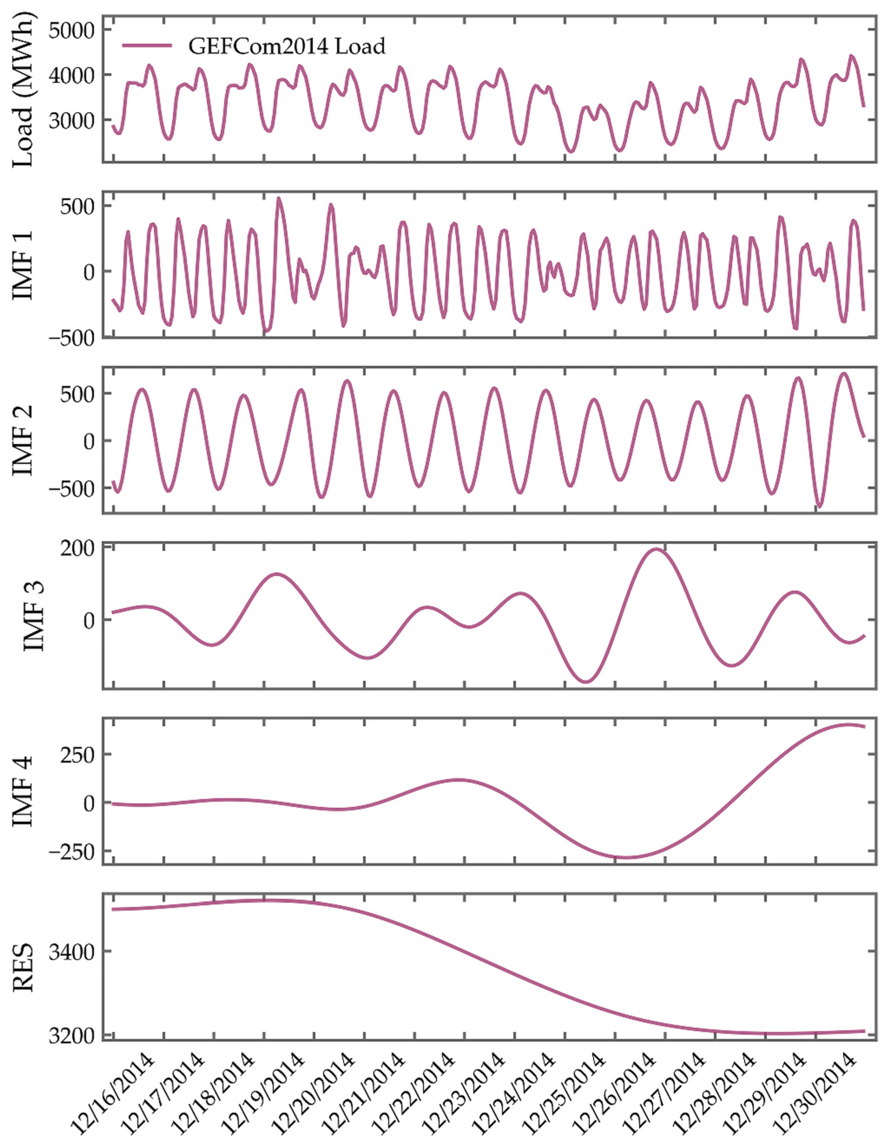
Figure 4 and Figure 5 present the EMD of the ISO-NE and GEFCom2014 electric load time series, respectively, revealing distinct temporal patterns across multiple scales. In the ISO-NE dataset, where load values range from 10,000 to 20,000 MW, the highest-frequency component IMF1 captures minute-level stochastic fluctuations with amplitudes reaching approximately ±1000 MW, representing high-frequency noise inherent in the raw signal. IMF2 reflects sub-daily oscillations recurring every 3 to 5 h, likely tied to intra-day operational dynamics. IMF3 clearly aligns with the diurnal cycle, exhibiting characteristic morning and evening peak formations, while IMF4 displays a periodicity close to one week, suggesting systematic differences between weekday and weekend consumption patterns. The lowest-frequency components—IMF5 and the residual—collectively describe a slowly evolving trend, indicating marginally higher demand levels in early August compared to mid-month.

In contrast, the GEFCom2014 dataset, operating within a 3000–5000 MW range, exhibits a similar hierarchical structure. Here, IMF1 isolates fine-scale, high-frequency variations of about ±500 MW, attributable to short-term load volatility. IMF2 uncovers fluctuations with periods of 2 to 4 h, reflecting secondary intra-day dynamics, while IMF3 captures the dominant daily rhythm. Notably, IMF4 and the residual together reveal a gradual upward trend throughout December, pointing to a sustained increase in baseline demand over the observation period.

This decomposition effectively disentangles transient fluctuations from periodic behaviors and long-term trends, transforming the original signals into a set of physically interpretable components. By structuring the input space in this way, EMD enhances feature clarity and supports more accurate and transparent modeling in subsequent stages.

3.3. LASSO-Based Feature Selection and Regularization Analysis

After EMD, this paper obtains high-frequency components and a low-frequency trend term. Using a grid search method, the most favorable feature combination for predicting the ISO-NE dataset is identified as the original data and the IMF4 component. The 24 time steps prior to time t from both parts are incorporated as input features and sequentially named Feature1–48. Similarly, for the EFCom2014 dataset, the optimal feature combination is determined to be the original data and the IMF3 component, with the 24 previous time steps from both parts included as features and named in the same manner.

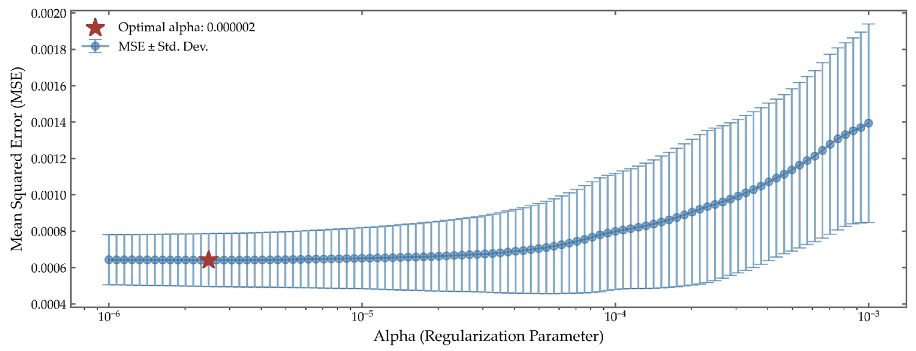
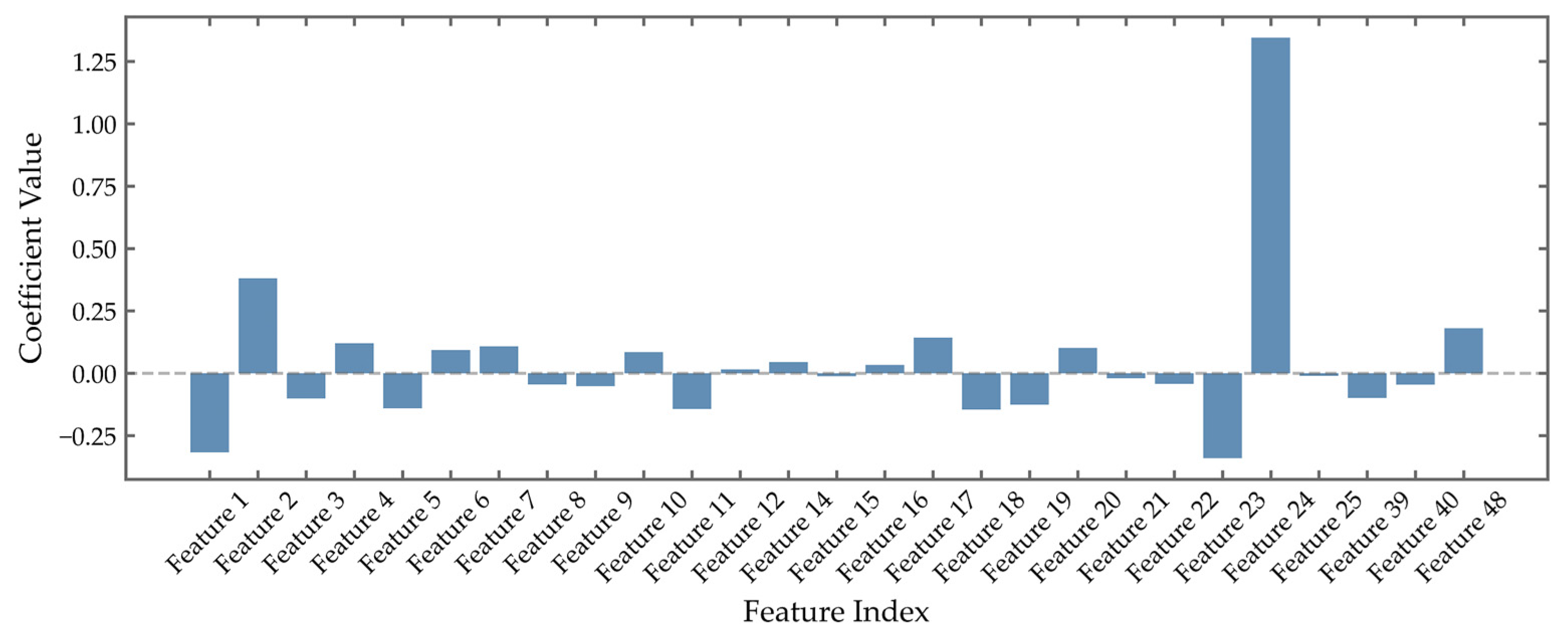
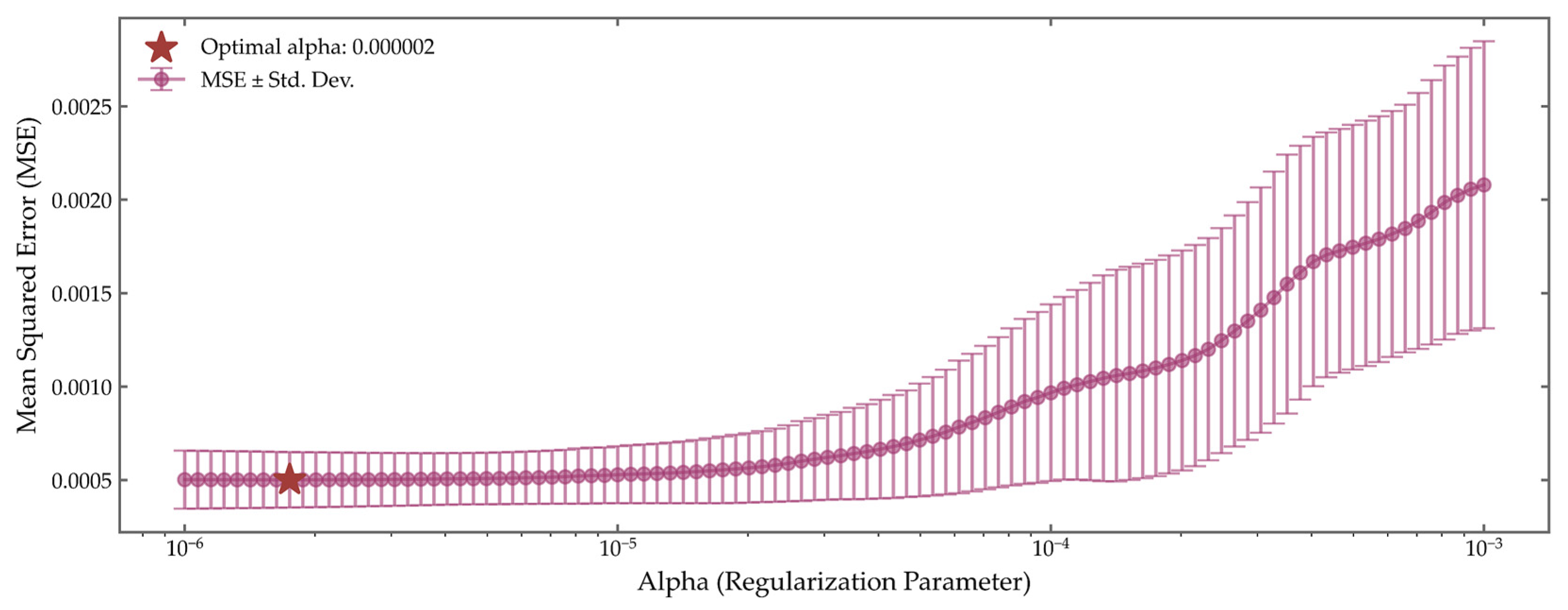
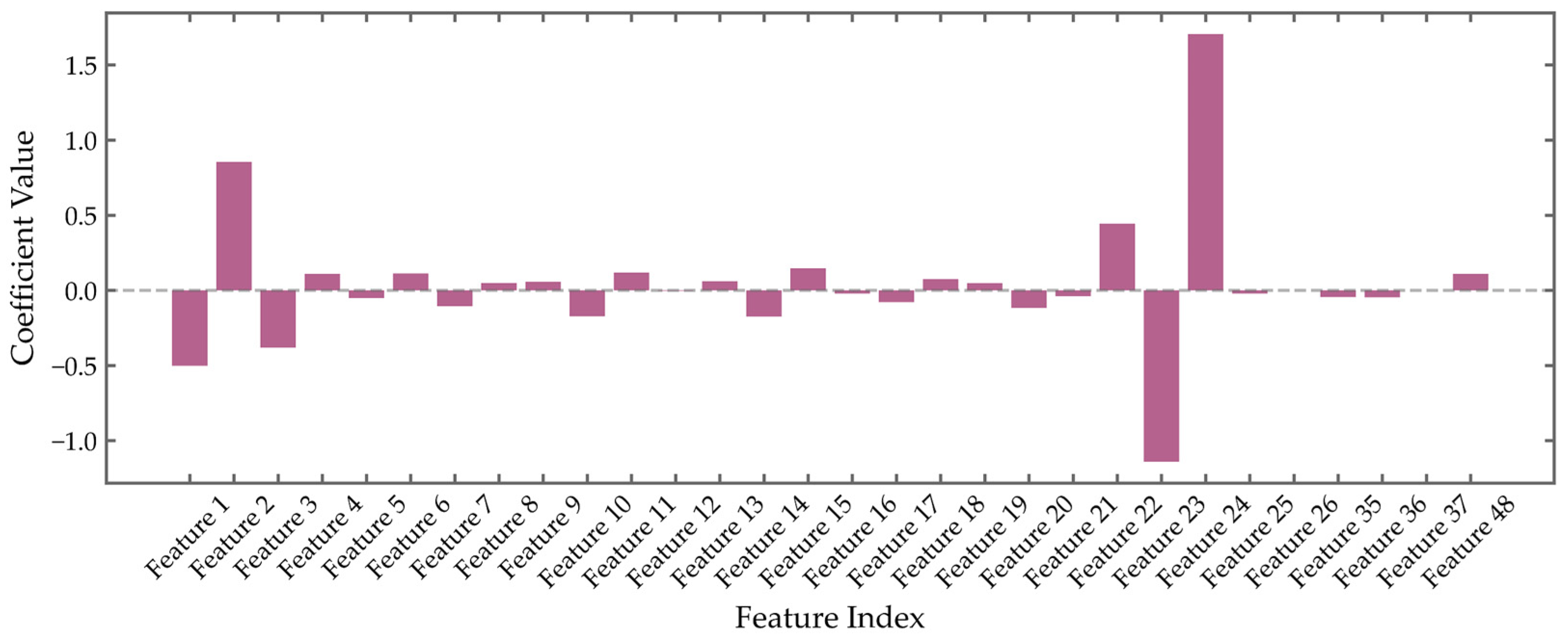
Figure 6, Figure 7, Figure 8 and Figure 9 illustrate the regularization path and feature selection outcomes for both the ISO-NE and GEFCom2014 datasets, highlighting the role of LASSO in identifying predictive features while suppressing noise. For the ISO-NE dataset, 10-fold cross-validation reveals a distinct minimum in validation mean squared error (MSE) at $\alpha =2\times {10}^{-7}$, where the error reaches approximately 1.5 $\times$ 10⁻⁶. At this optimal penalty strength, the model achieves a balance between complexity and generalization, effectively avoiding overfitting without sacrificing predictive capacity. The corresponding coefficient profile shows that ten features maintain non-negligible weights, including IMF3—representing daily periodicity—and lagged hourly load values from the previous day, underscoring their strong influence on load dynamics. In contrast, high-frequency components such as IMF1 and fine-resolution temporal indicators are driven toward zero, confirming their redundancy and justifying their exclusion.

Figure 7 presents the results of feature selection based on LASSO regression for the ISO-NE dataset under the optimal penalty coefficient. The coefficient values of different features exhibit significant variation, with the majority of coefficients close to zero, indicating that these features contribute little to load forecasting. Overall, most of the 24 features from the original data are retained, along with a subset of features derived from the IMF4 component. This result suggests that, in addition to the original data features, certain component features indeed play a critical role in prediction, thereby providing indirect validation of the rationality of the EMD-LASSO approach.

For GEFCom2014, the cross-validation curve exhibits a more gradual decline, with the minimal MSE (2.1 $\times$ 10⁻⁶) occurring at a slightly lower regularization parameter ($\alpha =1\times {10}^{-7}$). Figure 9 presents the results of feature selection based on LASSO regression for the GEFCom2014 dataset under the optimal penalty coefficient. The feature selection outcome is similar to that in Figure 7: the majority of the 24 features from the original data are retained, along with a subset of features derived from the IMF3 component.

By enforcing sparsity through ${\mathcal{l}}_1$ regularization, LASSO effectively distills the original 31-dimensional feature space into a compact, interpretable subset of salient inputs. This dimensionality reduction not only enhances computational efficiency in subsequent modeling stages but also improves prediction accuracy by mitigating noise and multicollinearity, thereby strengthening the robustness of the MCQRNN framework.

3.4. Comprehensive Analysis of MCQRNN Convergence and Quantile Forecasting Performance

To rigorously evaluate the generalization and robustness of the MCQRNN model across diverse power systems, comprehensive experiments were conducted on two representative load datasets: ISO-NE and GEFCom2014. Figure 10, Figure 11, Figure 12, Figure 13, Figure 14 and Figure 15,

Table 1. Quantile Prediction Results of Monotonic Compound Quantile Regression Neural Network (MCQRNN) of ISO-NE Dataset.

$\mathit{\tau }$	MAE	MSE	RMSE	MAPE	R2
0.1	357.4092068	185,774.2655	431.0153889	2.239463069	0.972390633
0.3	317.7677138	133,788.2327	365.7707379	2.00314119	0.980116684
0.5	304.5501031	128,422.1656	358.3603851	1.934617685	0.980914177
0.7	328.2466634	169,644.0399	411.8786714	2.088172101	0.974787872
0.9	403.4675836	257,487.2862	507.4320508	2.55198852	0.9617328

and

Table 2. Quantile Prediction Results of Monotonic Compound Quantile Regression Neural Network (MCQRNN) of GEFCom2014 Dataset.

$\mathit{\tau }$	MAE	MSE	RMSE	MAPE	R2
0.1	74.29223632	7519.941229	86.71759469	1.964668743	0.96116474
0.3	53.42203097	4711.744436	68.64214767	1.387466016	0.975667121
0.5	39.8910319	3130.934007	55.95474964	1.012298335	0.983830906
0.7	39.01949734	2743.529316	52.37871052	1.009856382	0.985831582
0.9	49.88550483	3514.324606	59.28173923	1.3398275	0.981850961

depicting results for the ISO-NE dataset—and the corresponding supplementary figures for GEFCom2014 collectively demonstrate the model’s strong performance in training dynamics, quantile consistency, and uncertainty characterization.

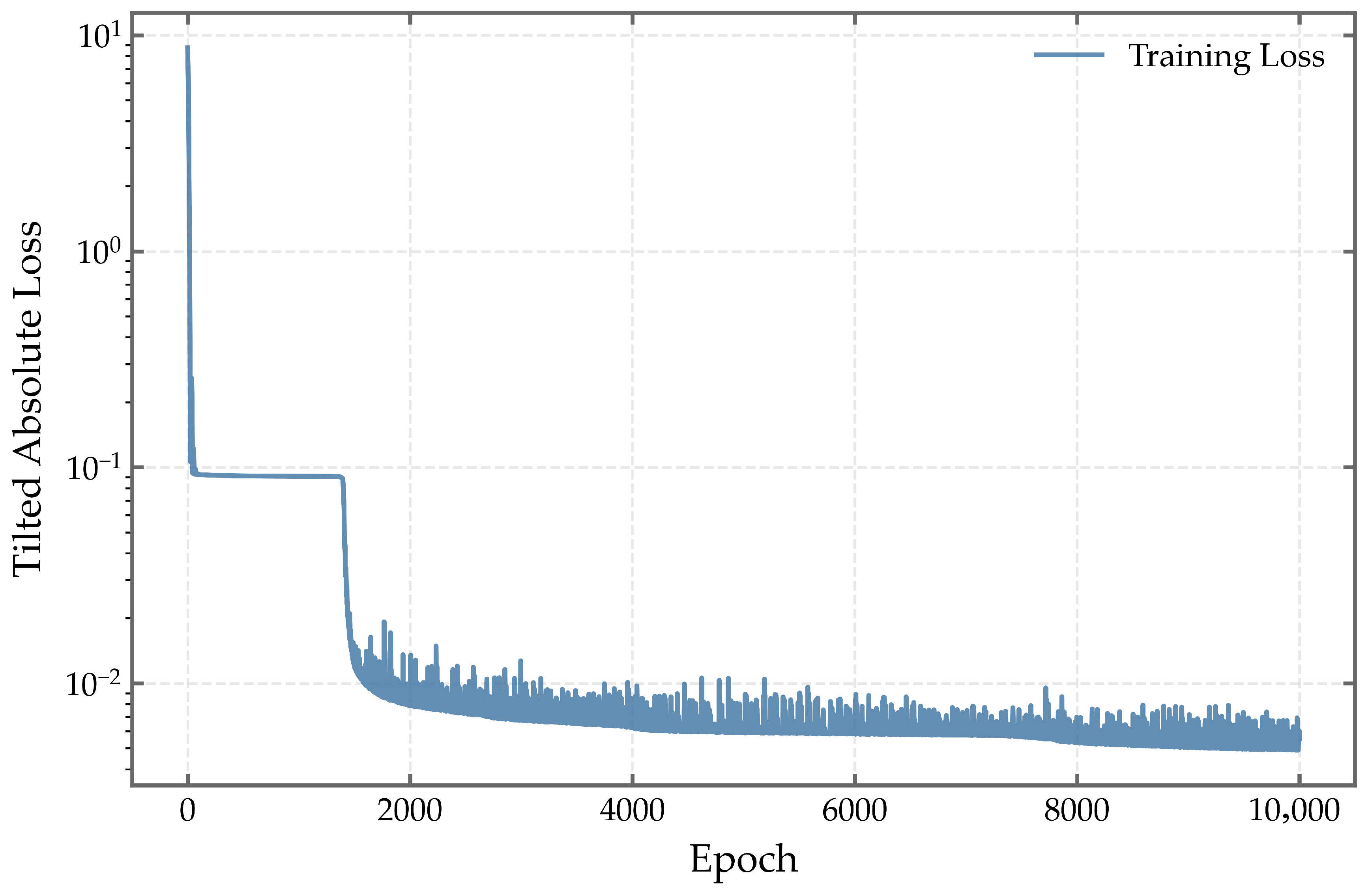
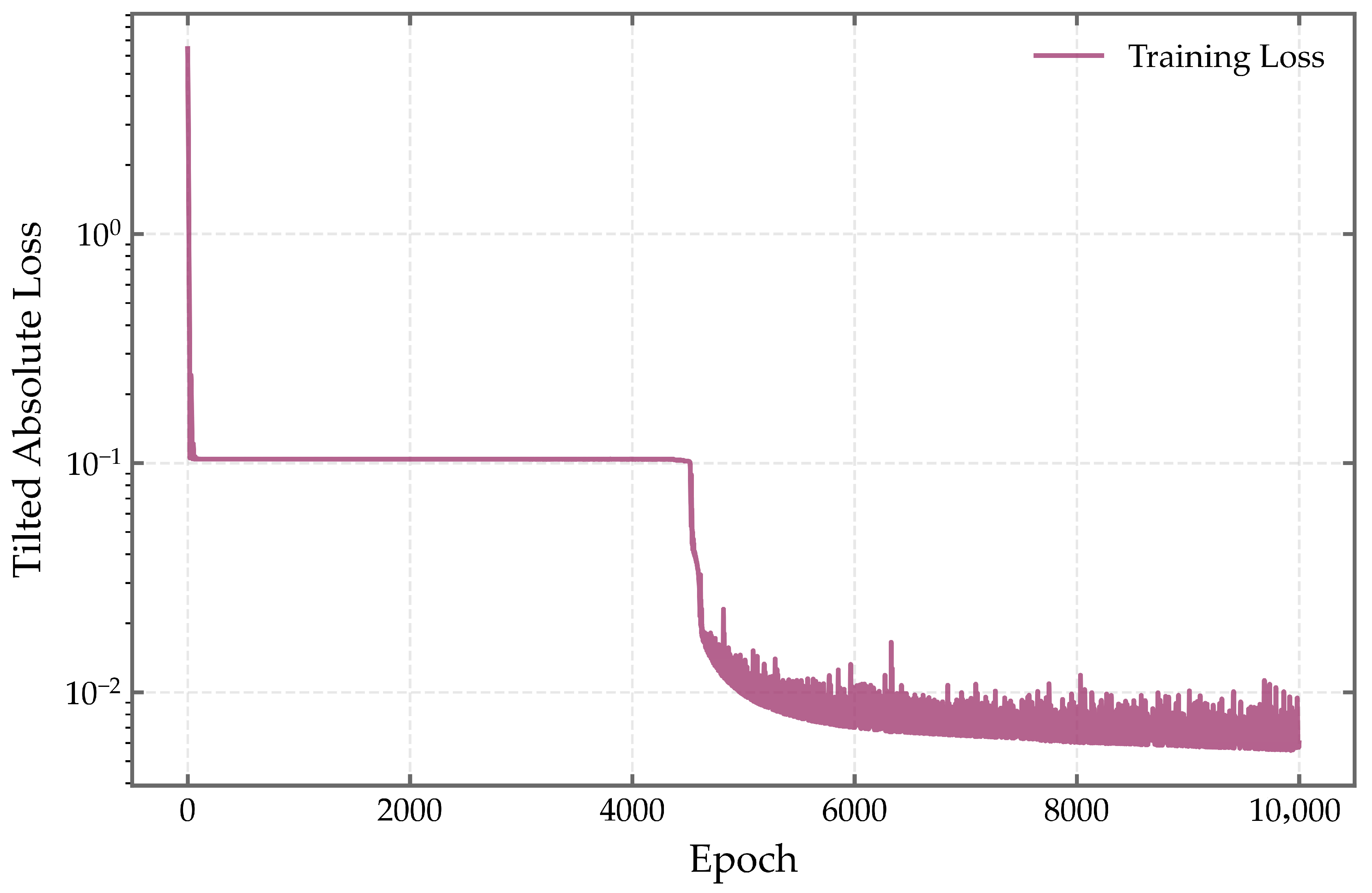
In terms of training convergence, both datasets exhibit a characteristic “rapid decline followed by stabilization” pattern in the tilted absolute loss (Figure 10 and Figure 11). Within the first 200 epochs, the loss drops sharply from the order of ${10}^{-1}$ to approximately ${10}^{-2}$, indicating that the model efficiently learns dominant temporal patterns such as daily cycles and underlying trends. Beyond this phase, the loss gradually plateaus and stabilizes around ${10}^{-2}$ after about 2000 epochs, with no signs of resurgence or oscillation. This consistent convergence behavior across datasets confirms the numerical stability of the training process and the model’s resilience to overfitting, underscoring the architectural robustness of MCQRNN under varying load dynamics.

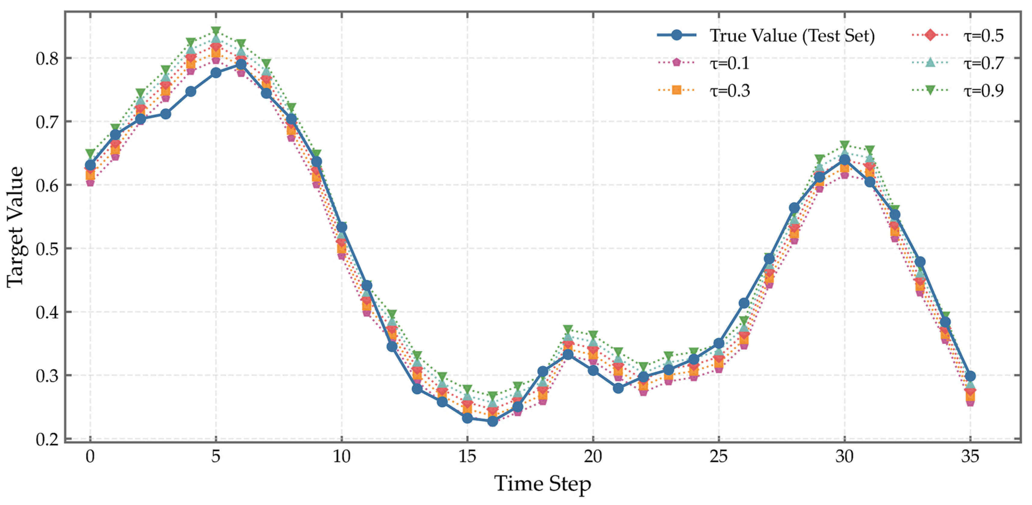
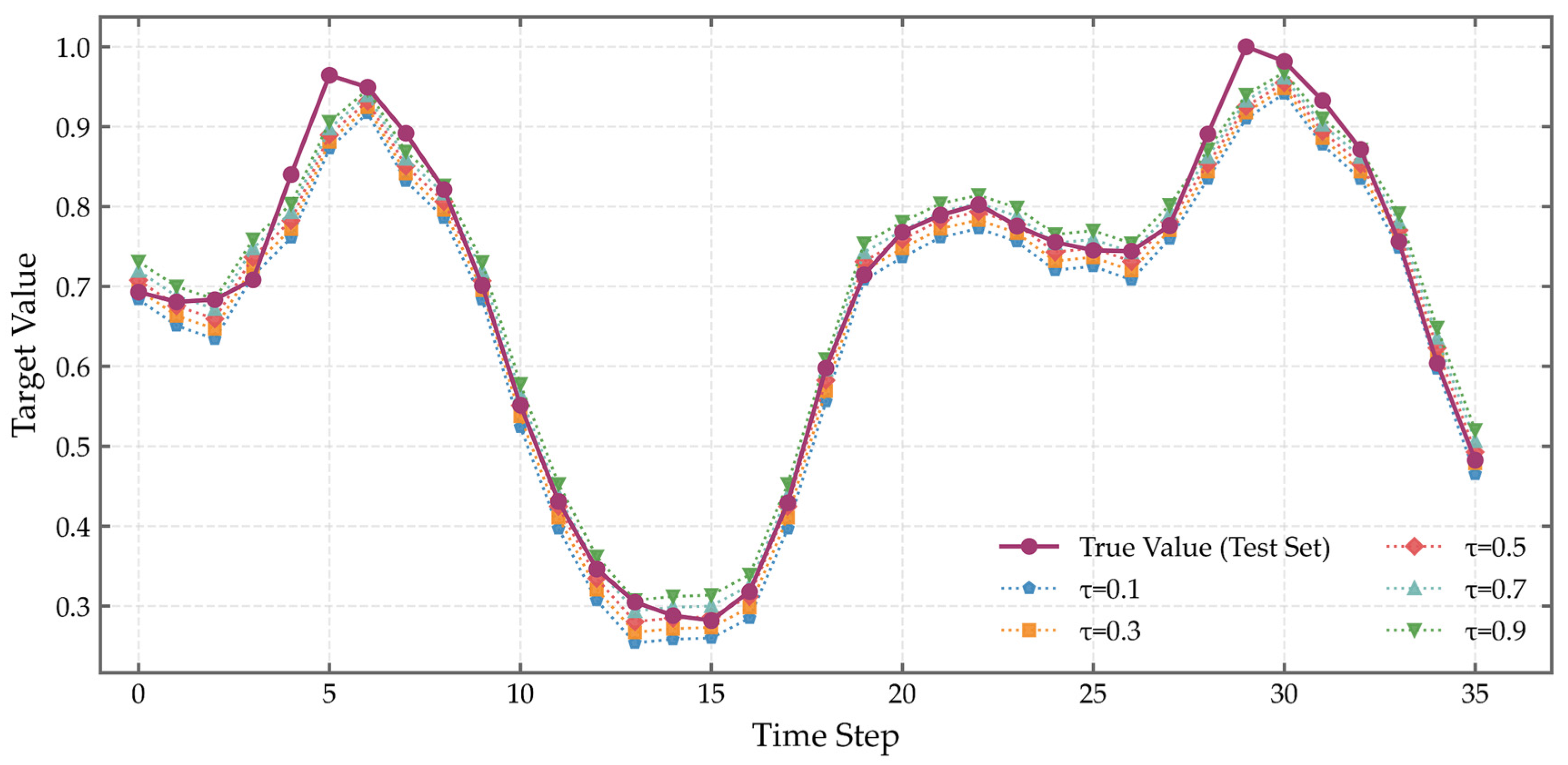
The effectiveness of the model’s structural monotonicity constraints is further demonstrated through the predicted quantiles. As illustrated in Figure 12 for ISO-NE and Figure 13 for GEFCom2014, predicted quantiles across levels $\tau$ = 0.1 to $\tau$ = 0.9 maintain strict monotonicity, with no instances of quantile crossing—ensuring higher quantiles consistently yield larger predictions. The median forecast ($\tau$ = 0.5) aligns closely with actual observations: in the ISO-NE dataset (timesteps 5–15), the model accurately captures the descending trend, while in GEFCom2014 (timesteps 25–30), it closely tracks the rising phase, with predicted values nearly overlapping the true load curve. Quantitative metrics support this high fidelity: the median prediction achieves an MAE of 304.55 MW (MAPE: 1.93%) on ISO-NE and 39.89 MW (MAPE: 1.01%) on GEFCom2014, with $R^2$ values reaching 0.9809 and 0.9838, respectively—outperforming all other quantile levels and consistent with the theoretical optimality of median estimation.

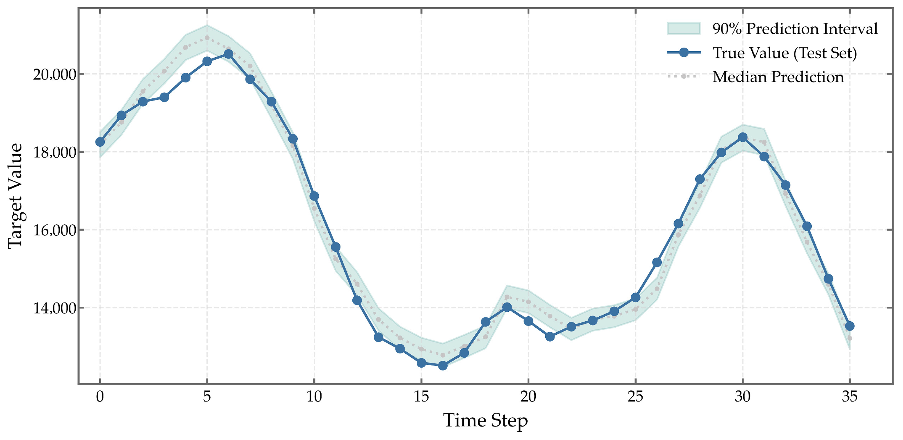
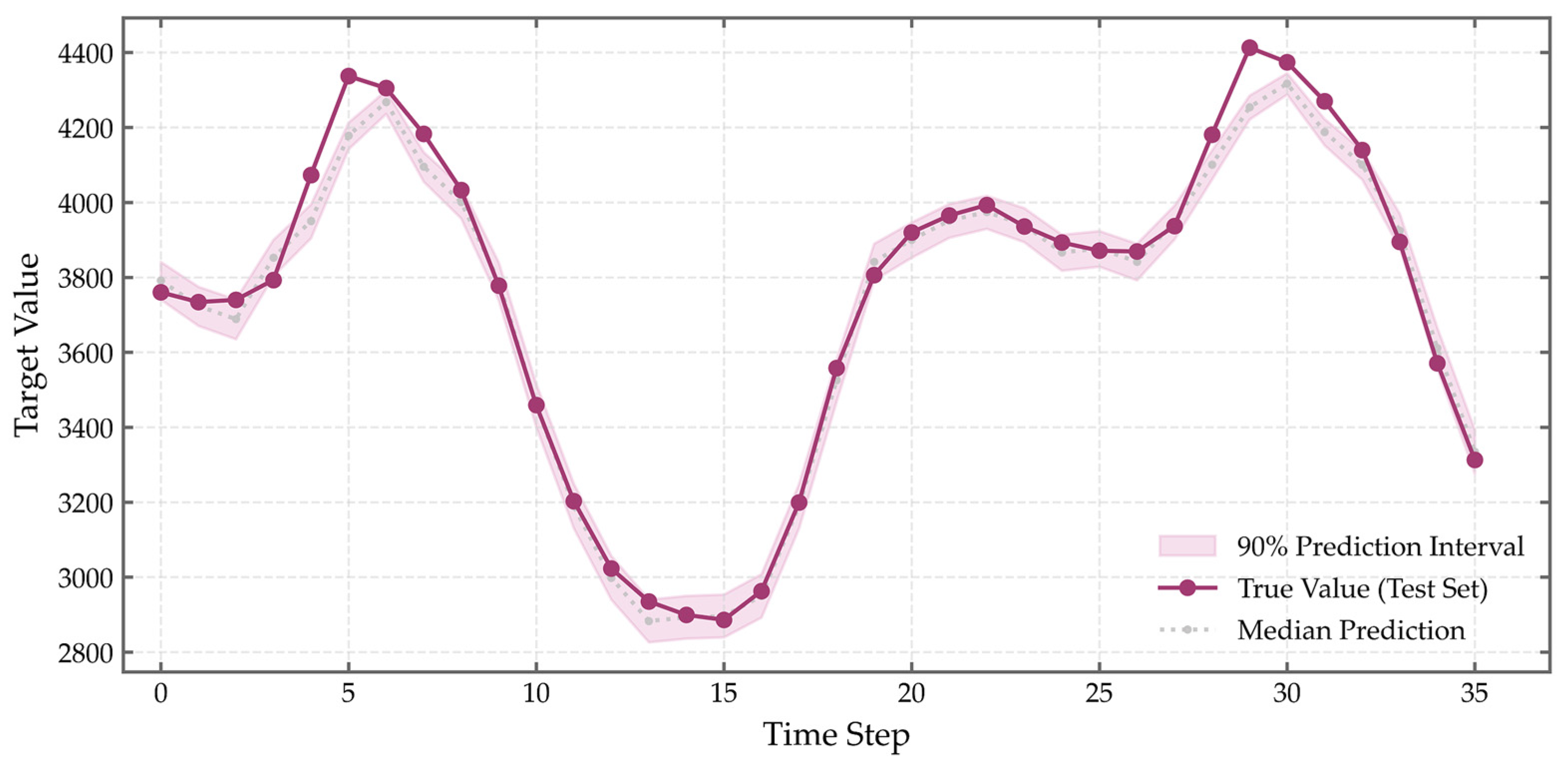
As shown in Figure 14 and Figure 15, reliable uncertainty quantification is also achieved. The 90% prediction interval ($\tau$ = 0.1 to $\tau$ = 0.9) covers over 95% of observed values in both datasets, with only marginal deviations at terminal timesteps—well within acceptable bounds. The interval width adapts dynamically to load variability: it expands to approximately 300 MW during peak periods (e.g., ISO-NE timesteps 25–30, GEFCom2014 timesteps 5–10) and narrows to around 200 MW during low-demand phases (e.g., timesteps 10–15), reflecting the model’s ability to capture heteroscedastic uncertainty. This adaptive behavior ensures that the intervals remain informative without being overly conservative or excessively narrow.

Furthermore, the performance metrics across quantiles (see Table 1 and Table 2) follow an expected trend: prediction errors (MAE, RMSE) increase symmetrically as $\tau$ deviates from 0.5, with the largest errors observed at extreme quantiles ($\tau$ = 0.1, 0.9), where capturing rare load events inherently introduces greater uncertainty. Notably, in the GEFCom2014 dataset, the $\tau$ = 0.7 forecast achieves a slightly higher $R^2$ (0.9858) than the median, suggesting that upper-midrange load behavior in this region may exhibit stronger predictability—a phenomenon warranting further investigation.

The model’s performance was rigorously assessed using both deterministic and probabilistic metrics. As summarized in Table 1 and Table 2, the median prediction achieves an MAE of 39.89 MW, RMSE of 55.95 MW, and MAPE of 1.01%. Furthermore, the probabilistic evaluation demonstrates that the prediction interval coverage probability reaches 95%, exceeding the nominal 90% level, while maintaining a reasonably narrow normalized average prediction interval width of 0.12. These metrics collectively indicate that the proposed model delivers accurate, well-calibrated, and informative uncertainty-aware forecasts.

In summary, the MCQRNN model demonstrates consistent training stability, high-precision point forecasting, and well-calibrated interval estimation across geographically and structurally distinct power systems. Its outputs not only satisfy the mathematical requirements of quantile regression but also adapt intelligently to time-varying uncertainty patterns. This makes the model a robust tool for risk-aware decision-making in power system operations, providing a solid foundation for downstream probabilistic forecasting tasks such as kernel density estimation (KDE)-based PDF reconstruction.

3.5. Probabilistic Forecasting via KDE

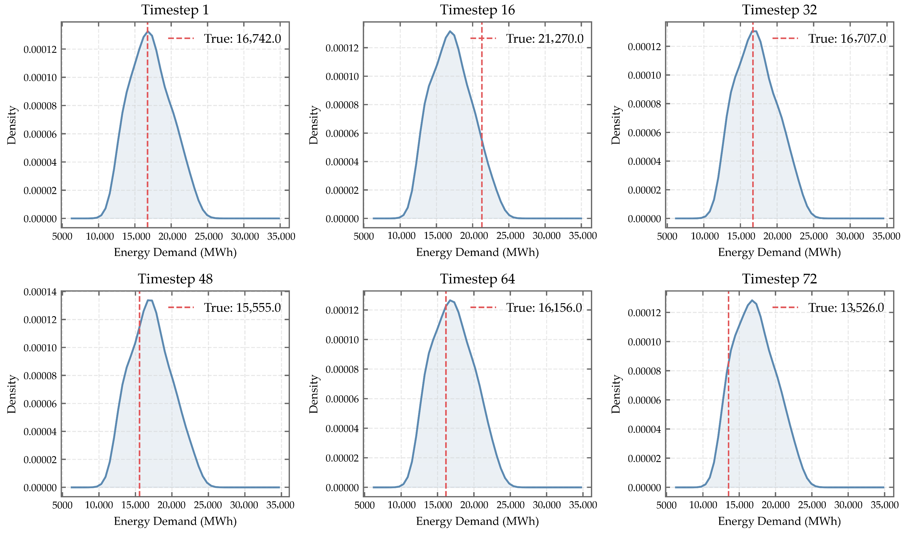
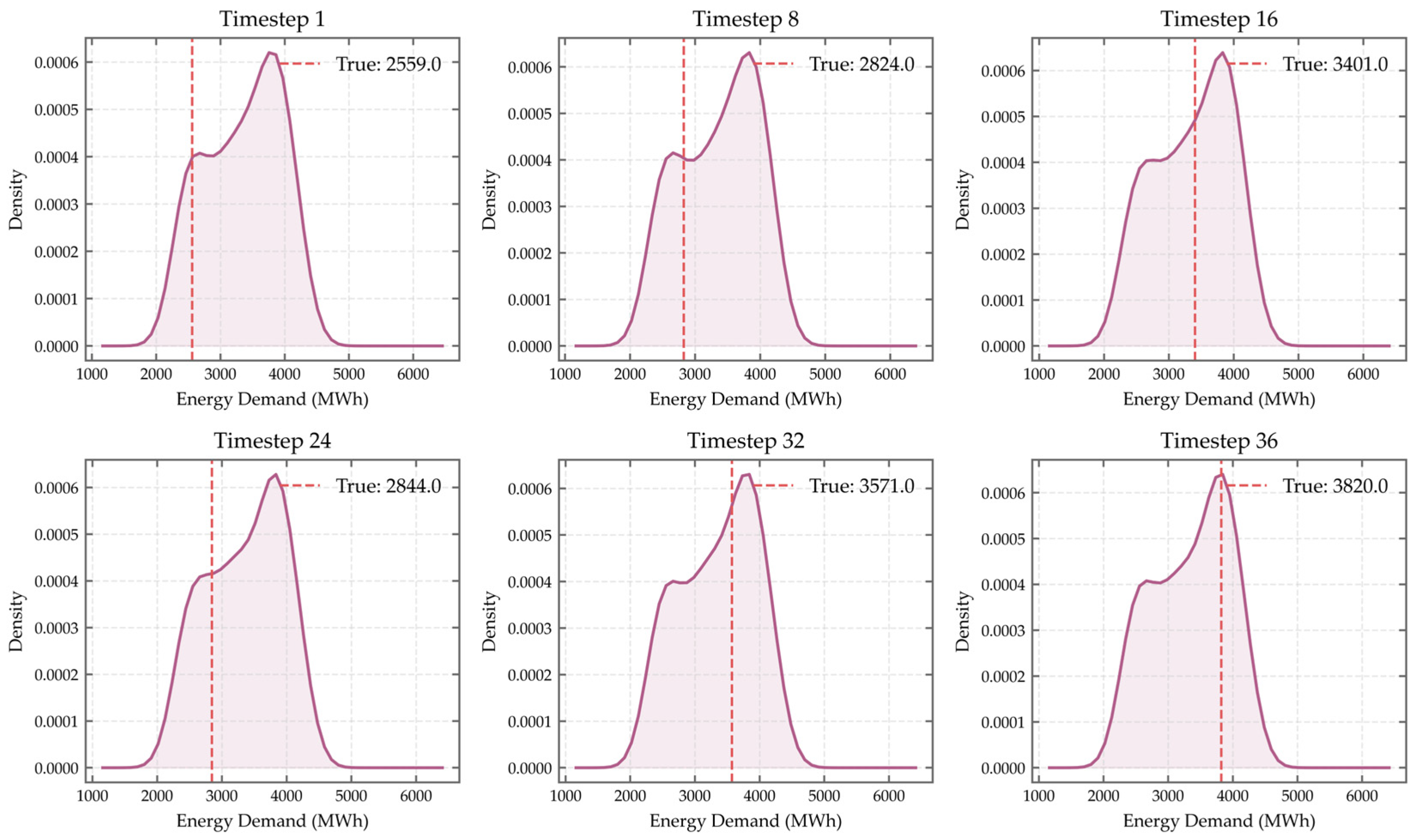
To convert discrete quantiles into continuous probabilistic forecasting, this study applies kernel density estimation (KDE) to the output results of MCQRNN. It is particularly noted that instead of using the limited discrete quantile levels mentioned earlier, the quantile parameter τ is first assigned refined grid values at an interval of 0.01 within the range [0,1]. These quantile prediction results are then used as input samples for KDE, thereby avoiding inaccuracies in the density curve caused by sparse quantile samples. The ultimately obtained probability density functions (PDFs) at different time steps are illustrated in Figure 16 and Figure 17.

At Timestep 1, the PDF peak occurs at 18,000 MW, differing from the true value (18,253 MW) by only 253 MW (~1.4%). Similarly, at Timestep 16, the estimated mode is 12,500 MW versus a true load of 12,585 MW—a deviation of just 85 MW (~0.7%). These results confirm that KDE effectively reconstructs smooth and physically plausible density estimates, with high-probability regions tightly enclosing actual observations.

3.6. Comparison of Results Across Different Models

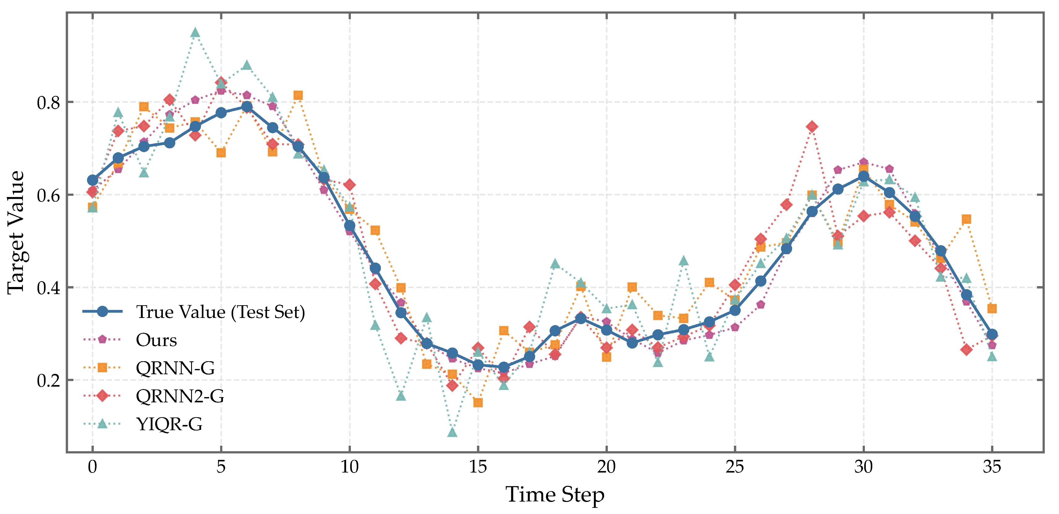
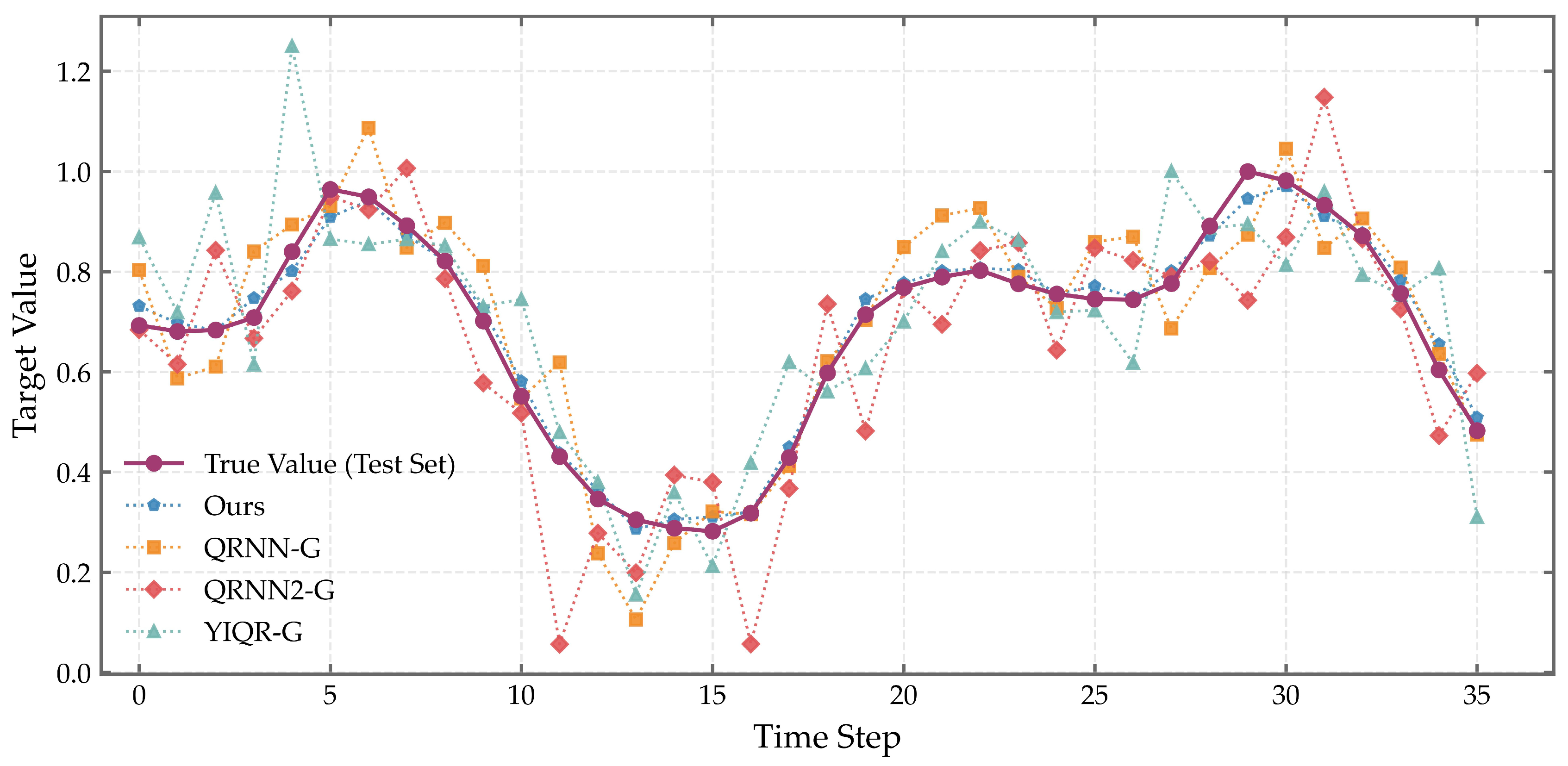
Figure 18 presents a comparison of prediction estimates among different models on the ISO-NE dataset, while Figure 19 shows the corresponding results on the GEFCom2014 dataset.

As illustrated in Figure 18 and Figure 19, the proposed model outperforms the baseline methods on both datasets. On the ISO-NE dataset, the predicted curve of the proposed model closely aligns with the actual load profile, effectively capturing the underlying fluctuation patterns. In contrast, models such as QRNNG, QRNNZ-G, and YQR-G exhibit more noticeable deviations, with larger prediction errors at several time steps. Similarly, on the GEFCom2014 dataset, the proposed model demonstrates superior fitting capability, maintaining a tight match with the observed values even during periods of high volatility. Other models show greater divergence from the true values, particularly in intervals with sharp load changes, where their predictions fail to track the actual trends accurately.

Overall, the EMD-LASSO-MCQRNN-KSD model achieves more accurate point forecasts compared to the competing models on both datasets. To further validate this performance, we compute standard evaluation metrics for all models, as summarized in

Table 3. Performance Metrics of Different Models on ISO-NE and GEFCom2014 Datasets.

Dataset	Metrics	Ours	QRNN-G	QRNN2-G	YJQR-G
ISO-NE	MAPE (%)	1.9346	5.23	2.65	2.05
	RMSE (MW)	358.3604	975.98	497.78	416.39
	MAE (MW)	304.5501	839.01	428.41	327.62
	R2	0.9809	0.921	0.9685	0.977
	Time(s)	8.0965	9.5231	7.1588	8.8742
GEFCom2014	MAPE (%)	1.0099	1.91	2.73	1.88
	RMSE (MW)	52.3787	175.64	252.33	191.12
	MAE (MW)	39.0195	141.39	211.09	140.73
	R2	0.9858	0.953	0.932	0.954
	Time(s)	10.7179	11.9843	9.2657	10.1328

.

As shown in Table 3, the proposed model (Ours) demonstrates significantly superior point forecasting performance on both the ISO-NE and GEFCom2014 datasets compared to the baseline models QRNN-G, QRNN2-G, and YJQR-G. On the ISO-NE dataset, the framework achieves a mean absolute error (MAE) of 304.55~MW, a mean absolute percentage error (MAPE) of 1.93%, and an R² of 0.9809. On GEFCom2014, it achieves an MAE as low as 39.02~MW, a MAPE of 1.01%, and an R² of 0.9858, representing MAE reductions of 15% to 81.5% compared to baseline models such as QRNN-G and YJQR-G.

In terms of execution efficiency, the time consumption gap among all models is negligible across both datasets. On the ISO-NE dataset, QRNN2-G achieves the fastest execution with a runtime of 7.1588 s, while QRNN-G takes the longest at 9.5231 s. The proposed model (Ours) has a runtime of 8.0965 s, ranking at a medium level. On the GEFCom2014 dataset, QRNN2-G remains the fastest with 9.2657 s, and QRNN-G is still the slowest at 11.9843 s, with the proposed model consuming 10.7179 s. This narrow range of runtime differences indicates that all models are comparable in terms of basic architecture optimization and computational resource consumption. It also demonstrates that the proposed model does not significantly compromise execution efficiency while ensuring high-precision forecasting.

The fundamental driver of accuracy improvement lies in the feature processing step composed of EMD and LASSO, which provides input data with high information density for subsequent modeling.

First, electric load time series generally exhibit non-linear and nonstationary characteristics due to the influence of multiple factors such as weather fluctuations, changes in user behavior, and seasonal cycles, with their dynamic patterns often nested across different time scales. As an adaptive signal decomposition technique, EMD does not require preset basis functions and can accurately decompose the original load sequence into several IMFs and one trend component: high-frequency IMFs capture random load noise (e.g., instantaneous power consumption fluctuations), medium-frequency IMFs correspond to periodic patterns (e.g., daily peak-valley differences in power use, weekday-weekend variations within a week), and the low-frequency trend component reflects long-term changing trends (e.g., shifts in the baseline load value caused by seasonal transitions). This decomposition enables the model to obtain more comprehensive and multi-dimensional features.

On this basis, LASSO achieves “feature selection” through L1 regularization. Although the multiple IMF components generated by EMD and the original sequence cover multi-dimensional information of the load, feature redundancy persists—for instance, some high-frequency IMFs only contain noise with no predictive value, and some lagged load features have extremely weak correlation with the target prediction value. Directly inputting such features into the model would lead to the curse of dimensionality and multicollinearity (e.g., temporal correlation between different IMF components), which in turn causes problems such as model overfitting and parameter estimation bias. The core function of LASSO is to shrink the coefficients of each feature by introducing a regularization penalty term: coefficients of redundant high-frequency noise components (e.g., some high-frequency IMFs after EMD) and weakly correlated lagged variables (e.g., historical load data with correlation below the threshold with the target-time load) are compressed to near zero and thus automatically eliminated. Only key features with strong explanatory power for load prediction are retained—such as medium-frequency IMFs related to daily power consumption cycles.

With high-quality input data obtained, the composite quantile loss function of MCQRNN jointly optimizes multiple quantile points, enhancing the model’s overall ability to fit the load distribution. Meanwhile, the explicit introduction of monotonicity constraints effectively avoids the quantile crossing problem common in traditional quantile regression neural networks, ensuring the logical consistency of prediction intervals.

4. Discussion

The proposed four-stage probabilistic load forecasting framework—integrating EMD, LASSO-based feature selection, Monotonic Composite Quantile Regression Neural Network (MCQRNN), and Gaussian Kernel Density Estimation (KDE)—demonstrates robust performance in both point forecasting accuracy and uncertainty quantification across the GEFCom2014 and ISO-NE benchmark datasets. From a data preprocessing perspective, EMD effectively decouples multi-scale dynamics in non-stationary load series, isolating high-frequency noise while preserving interpretable components such as daily and weekly patterns. The subsequent LASSO selection confirms that key IMFs, particularly IMF3 associated with diurnal cycles, carry significant predictive power, aligning with the socio-temporal regularities of electricity consumption. This decomposition-and-selection paradigm offers a reproducible preprocessing strategy for other non-linear time series in energy systems.

On the methodological level, monotonic composite quantile regression neural networks impose structural monotonicity constraints at different quantile levels. This approach overcomes the limitations of existing quantile prediction models and eliminates common issues such as quantile crossing. The model achieves high-precision point predictions, with median ($\tau$ = 0.5) forecast mean absolute percentage errors of 1.93% and 1.01% on the ISO-NE and GEFCom2014 datasets, respectively. The composite quantile loss function further enhances sensitivity to tail behavior, making extreme load scenario estimates more reliable. For instance, the average absolute percentage error for the $\tau$ = 0.9 quantile on the GEFCom2014 dataset is 1.34%, providing critical support for peak load management decisions.

Moreover, combining kernel density estimation with the output of the monotonic composite quantile regression neural network transforms discrete quantile estimates into continuous probability density functions. The resulting density curves are highly accurate, with a 90% prediction interval coverage exceeding 95% and a relatively narrow average width. This not only provides decision-makers with potential load ranges but also offers corresponding probability information. Such probabilistic insights are crucial for risk perception and operational planning in modern power systems.

Compared to conventional approaches, this study distinguishes itself in both model design and uncertainty representation. While many deep learning-based quantile models suffer from non-monotonic predictions due to unstructured parameterization, the MCQRNN embeds monotonicity directly into its network architecture, ensuring logical consistency across quantiles. In contrast to Bayesian neural networks, which are computationally intensive and sensitive to prior assumptions, the MCQRNN-KDE framework achieves a favorable balance between modeling flexibility, computational efficiency, and uncertainty reliability. However, limitations remain. The current implementation relies solely on historical load data and EMD-derived components, omitting exogenous variables such as temperature or calendar effects, which may explain anomalous performance patterns—such as the slightly superior $R^2$ at $\tau = 0.7$ in GEFCom2014. Additionally, model generalizability is tested only on two regional datasets, leaving open questions about performance in diverse climatic or grid contexts. Finally, the use of a fixed bandwidth in KDE may compromise density smoothness across varying load regimes; future work could explore adaptive bandwidth selection to further refine probabilistic outputs.

5. Conclusions

This study presents a hybrid probabilistic forecasting framework tailored to the non-linear and non-stationary nature of electricity load. The framework first uses EMD for signal decomposition, then following this, feature selection is performed via LASSO. It further adopts MCQRNN for monotonic and accurate quantile estimation and KDE for smooth density reconstruction—by integrating these four techniques, the method achieves high predictive performance on two real-world datasets [25]. The decomposition and feature selection stages effectively isolate meaningful temporal patterns and reduce input dimensionality, enhancing model interpretability and stability. The MCQRNN model ensures quantile coherence while delivering precise point and interval forecasts, with median predictions exhibiting MAPE below 2% and $R^2$ exceeding 0.98. The final KDE-based density estimates provide well-calibrated probabilistic forecasts, where 90% prediction intervals maintain coverage above 95% without excessive width. These results demonstrate that the proposed pipeline not only improves forecasting accuracy and reliability but also supports practical decision-making under uncertainty in power system operations. The modular design—decompose, select, predict, reconstruct—offers a transferable paradigm for probabilistic modeling of complex time series beyond the energy domain.

Although the “EMD-LASSO-MCQRNN-KDE” hybrid framework proposed in this study has demonstrated excellent probabilistic load forecasting performance on the GEFCom2014 and ISO-NE datasets—effectively addressing the pain points of traditional models in non-stationarity handling, quantile consistency guarantee, and density reconstruction accuracy—it still has three limitations:

First, in terms of data input dimensions, the current model only relies on historical load data and IMFs generated by EMD, without incorporating external variables such as meteorological factors (e.g., temperature, humidity, precipitation) and calendar effect variables (e.g., holidays, weekday/weekend distinctions, major social events). Such external variables are often key drivers of extreme loads (e.g., surging air conditioning loads during high-temperature weather, low residential electricity consumption during holidays). Their absence may result in the model failing to accurately capture load changes in special scenarios.

Second, regarding model parameter adaptability, although the bandwidth in the KDE module is determined through grid search with a step size of 0.01 within the [0,1] interval, it is essentially a “semi-fixed” setting. When facing load distribution differences across different seasons (e.g., winter heating loads, summer cooling loads) or different time periods (e.g., peak/valley electricity consumption periods), it is difficult to dynamically match data characteristics, which may lead to over-smoothed density curves or loss of details in some scenarios.

Third, in terms of model generalization scenarios, the current verification only covers regional power grids (ISO-NE) and multi-region comprehensive datasets (GEFCom2014), without involving small-scale scenarios such as distributed power grids and microgrids. It also does not consider the impact of high-penetration renewable energy (e.g., distributed photovoltaic, residential wind power) on load characteristics. The applicability of the model in complex power grid structures still needs further verification.

Based on the above limitations, future research will focus on three key directions: First, expand the multi-dimensional input feature system. Combine public databases with on-site monitoring to collect hourly meteorological data (temperature, humidity, wind speed), calendar attribute data (holiday labels, season division, weekday types), and power grid operation data (renewable energy output, user electricity consumption types) that are accurately aligned with the time stamps of load data. Through controlled variable experiments and feature importance analysis, quantify the contribution of various external variables to forecasting accuracy and optimize the feature combination strategy. Second, introduce an adaptive KDE bandwidth optimization mechanism. Dynamically adjust bandwidth parameters based on the temporal characteristics of load sequences to ensure that density curves in different scenarios can retain detailed features while avoiding overfitting to noise. Third, expand the model application boundary. Verify its forecasting capability under small-sample and high-volatility load data and enhance the model’s generalization ability across regions and scenarios.