Article

Lightweight Design of Screw Rotors via an Enhanced Newton–Raphson-Based Surrogate-Assisted Multi-Objective Optimization Framework

1
College of Mechanical Engineering, Zhejiang University of Technology, Hangzhou 310023, China
2
Zhejiang Key Laboratory of Intelligent Manufacturing for Aerodynamic Equipment, College of Mechanical Engineering, Quzhou University, Quzhou 324000, China
3
Zhejiang Chentai Machinery Manufacturing Co., Quzhou 324000, China
*
Author to whom correspondence should be addressed.
Processes 2025, 13(12), 3779; https://doi.org/10.3390/pr13123779 (registering DOI)
Submission received: 13 October 2025 / Revised: 11 November 2025 / Accepted: 18 November 2025 / Published: 22 November 2025
(This article belongs to the Section Process Control and Monitoring)

Abstract

Traditional solid screw rotors suffer from excessive weight, structural redundancy, low material utilization, and high energy consumption, conflicting with the growing demand for efficient, sustainable manufacturing. To address these challenges, this study proposes a lightweight design method for hollow, internally supported male screw rotors that simultaneously enhances stiffness and static–dynamic performance. A parameterized structural model with four key design variables was established, and multi-physics simulations integrating fluid flow, heat transfer, and structural mechanics were conducted to obtain mass, maximum deformation, and first-order natural frequency. Based on these simulation results, a surrogate-assisted multi-objective evolutionary optimization framework was employed: an enhanced Newton–Raphson-based optimizer (SNRBO) was used to tune the extreme gradient boosting surrogate (XGBoost 1.5.2), and the tuned surrogate then guided the Nondominated Sorting Genetic Algorithm III (NSGA-III) to perform multi-objective search and construct the Pareto front. Compared with a conventional solid rotor, the optimized design reduces mass by 64.43%, decreases maximum deformation by 4.41%, and increases the first-order natural frequency by 82.14%. These findings indicate that the proposed method provides an effective pathway to balance lightweight design with structural safety and dynamic stability, offering strong potential for green manufacturing and high-performance applications in energy, aerospace, and industrial compressor systems, and providing robust support for further advances in this field.

1. Introduction

With the continuous development of China’s machinery manufacturing industry, the concept of green manufacturing has become an important pathway to enhance industrial competitiveness. Screw air compressors, as essential power equipment, are widely applied in energy, aerospace, mining, petrochemical, and other fields due to their compact structure, high energy efficiency, and stable operation. The male rotor, as the core component, directly affects overall performance and efficiency. The design of conventional rotors is subject to three primary constraints: geometric limitations, such as the use of solid cores and uniform wall thickness, which hinder the optimization of internal material distribution; manufacturing process limitations, where traditional subtractive machining methods are inadequate for handling complex geometries, such as deep cavities and thin-walled structures, resulting in significant material waste and extended processing times; and energy efficiency and performance bottlenecks in the manufacturing process, including challenges related to effectively controlling residual stresses during heat treatment and ensuring assembly precision under high-speed operational conditions. These factors constrain the optimization of the rotor’s mass, stiffness, and dynamic performance [1]. As a result, existing design methods are no longer sufficient to meet the demands for high-efficiency, lightweight, and high-performance rotors, necessitating the development of new design approaches that integrate structural and process optimization.
Research on screw compressor optimization has focused mainly on modeling and parameter-based rotor optimization. For example, Li Y et al. [2] studied internal flow characteristics for structural enhancement; Ahmet et al. [3] and Dhayanandha, K et al. [4] applied the response surface methodology (RSM) to optimize depth, port, and injection parameters; Kaufmann, F et al. [5] proposed a generalized modeling approach; Zhao B et al. [6] studied thermo-leakage coupling using fuzzy beam finite elements; Tian Z Y et al. [7] derived rotor profile equations; Deng Z et al. [8] developed data-driven models; Kumar A et al. [9] combined Gaussian process regression with Bayesian optimization; Wang T et al. [10] applied back propagation (BP) neural network and genetic algorithm (GA) to the optimization of rotor profile parameters; Tran V et al. [11] adopted uniform design-based multi-objective optimization; Saravana et al. [12] performed conjugate heat transfer studies. Zhang Yongtao et al. [13] proposed honeycomb cavity rotors and fabricated them using 3D printing technology, achieving significant mass reduction while maintaining compressor performance, providing a new approach for lightweight rotor design.
In the field of hollow screw rotor lightweight design, some scholars have made attempts to reduce mass while preserving structural stiffness and dynamic performance, as detailed in the following studies. Chao Rui [14] analyzed equal-thickness hollow rotors with finite element simulations, showing significant mass reduction but decreased modal frequencies. Wang Zhibo [15] combined RSM with finite-element (FE) analysis for sequential optimization of wall thickness and support parameters, achieving mass reduction but limited to single-point solutions. Zhi Mingyu [16] proposed a shell–internal skeleton structure and optimized it through orthogonal tests with additive manufacturing, focusing on manufacturability but restricted to narrow parameter ranges. These efforts indicate that hollow rotor lightweight design has made initial progress, yet overall limitations remain, including locality, insufficient global exploration, and incomplete multi-objective trade-offs. A detailed comparison is presented in Table 1.
Beyond screw rotors, cross-domain studies further substantiate the broader value of multi-objective optimization for lightweight, high-performance rotating components. Bandini et al. developed a Computational Fluid Dynamics–Finite Element Method (CFD-FE) integrated topology-optimization workflow for a compressor blisk that unifies unsteady aerodynamic forcing with structural response and achieves about a 32% reduction in mass under dynamic constraints, demonstrating effective reconciliation of lightweighting and vibration performance [17]. This evidence supports positioning multi-objective methods as generally applicable tools across mechanical and aerospace structures, not solely within screw-compressor applications.
In recent years, surrogate-assisted optimization methods have gained attention. Wu et al. [18] proposed a framework that combines Bayesian optimization (BO), XGBoost and the Nondominated Sorting Genetic Algorithm II (NSGA-II) for building performance optimization; Liu Z et al. [19] verified its accuracy in hydrogen production design spaces; Han Y et al. [20] proposed a framework that combines the Synthetic Minority Over-sampling Technique (SMOTE) with XGBoost to address data imbalance; Mao F et al. [21] integrated XGBoost into evolutionary frameworks for expensive multi-objective problems. For hyperparameter optimization, Mehdary et al. [22], Fu J et al. [23], Zivkovic et al. [24], and Huang et al. [25] applied a genetic algorithm (GA), the Reference Vector Guided Evolutionary Algorithm (RVEA), and an improved Harris Hawks Optimization (HHO) method to enhance robustness; Lima Marinho et al. [26] applied meta-learning for hyperparameter selection. Qinghan L et al. [27] constructed a SHapley Additive exPlanations (SHAP)-XGBoost-based nonlinear mapping framework to address the T-shaped groove casing treatment design in transonic compressors; Jianping Wang et al. [28] combined XGBoost with GA for four-bar mechanism trajectory synthesis.
Meanwhile, the Newton–Raphson-based Optimizer (NRBO) has attracted attention due to its simplicity and fast convergence, as reported by Sowmya R et al. [29]. Applications of the NRBO include hyperparameter optimization for convolutional neural network (CNN)–least squares support vector machine (LSSVM), as explored by Huan B et al. [30], as well as the deep neural network (DNN) optimization utilizing non-dominated sorting and trap-avoidance operators, as demonstrated by Li Z et al. [31]. Further advancements have been made in improving robustness with dynamic inverse learning, Lévy flights, and Q-learning, as reported by Li Y et al. [32]. Additionally, chaotic initialization has been applied to broaden exploration, as shown by AbouOmar et al. [33], while Shi W et al. [34] introduced dynamic obstacle avoidance for path planning. Ni Y et al. [35] incorporated trust-region constraints with Lévy strategies, and Hou Z et al. [36] and Zeng H et al. [37] in 2025 focused on hyperparameter tuning for Transformer and TFT models. Lastly, Abazine et al. [38] proposed analytical initialization to achieve higher parameter precision. Despite these advancements, many of the improvements remain focused on operator-level modifications and lack a unified global optimization framework.
In summary, although previous studies have achieved certain results in modeling, surrogate construction, and optimization algorithms, there is currently a lack of systematic multi-objective optimization methods for the lightweight design of screw compressor male rotors. In response to this challenge, this paper proposes an enhanced NRBO algorithm (SNRBO) integrating multiple strategies, including attention-guided dimensional weighting, adaptive DF regulation, dynamic Lévy flight, an elite–exploration–regular layered population mechanism, a historical memory repository, and genetic crossover. This enhanced optimizer is used to train a high-precision XGBoost surrogate model and is coupled with the NSGA-III multi-objective evolutionary algorithm to optimize the parameters of the hollow support structure of the screw rotor. The proposed method achieves a significant reduction in rotor weight while maintaining structural strength and dynamic performance, offering an effective path for intelligent and green design of compressor core components.

2. Methods

2.1. Study Framework

To achieve lightweighting of screw rotors while satisfying stiffness and dynamic performance requirements, this paper proposes a three-objective synergistic optimization method based on multi-physics coupled simulation and an improved SNRBO-XGBoost-NSGA-III. This method is applied to the study of structural parameter optimization for hollow internally-supported male rotors. By simultaneously minimizing rotor mass and maximum total deformation while maximizing the first-order natural frequency, the proposed method seeks to achieve optimal parameter synthesis that substantially enhances both rotor performance and energy efficiency. The overall workflow of the proposed optimization framework is illustrated in Figure 1.
First, this paper selects four key geometric parameters of the hollow internally-supported male rotor, namely the thickness of the two end faces, the thickness of the working gear face, the width of the support rod, and the diameter of the support column, as optimization variables. Parametric modeling is carried out in SolidWorks 2023, and 180 structural samples are generated using the Latin hypercube sampling method. Subsequently, using the ANSYS 2022R1 platform, single-direction coupled simulations of flow, heat transfer, and structural mechanics are performed. The rotor mass, maximum total deformation, and first-order natural frequency are obtained for each sample, offering training data for constructing the predictive model.
During the modeling phase, the XGBoost regression algorithm is employed to construct predictive models for the three performance indicators. To improve the model’s generalization and fitting accuracy, the SNRBO algorithm, enhanced by multiple strategies, is introduced to adaptively optimize key XGBoost model hyperparameters, including num_trees, max_depth, etc. The SNRBO algorithm systematically incorporates six mutually reinforcing mechanisms: (1) a standard-deviation-weighted dimensional attention scheme to dynamically emphasize pivotal variables; (2) an adaptive DF regulation strategy employing a Sigmoid schedule to balance perturbation intensity in real time; (3) a Lévy-flight operator for long-range global exploration; (4) an elite–exploration–regular tripartite population structure that finely trades off exploitation and exploration; (5) an elite-replay memory repository for the continual refinement of inferior solutions; and (6) a GA-based co-evolutionary framework integrating crossover and non-uniform mutation for information recombination. This integrated paradigm markedly enhances convergence accuracy, robustness, and computational efficiency within high-dimensional, multimodal, and highly nonlinear search spaces.
Finally, the SNRBO-optimized XGBoost model is used as the fitness function to construct an NSGA-III multi-objective optimization model. This workflow follows a sequential execution mode: after the multi-objective optimization identifies the Pareto optimal candidates, each solution is verified through high-fidelity finite element simulations in ANSYS 2022R1. The simulation serves as a post-optimization validation step to ensure the physical accuracy and consistency of the predicted results. Once the simulation results confirm that the optimized designs meet the expected structural and dynamic performance requirements, the workflow is concluded. The sequential process ensures computational efficiency while maintaining strong agreement between optimization predictions and simulation outcomes.

2.2. Simulation Framework and Performance Indicators

2.2.1. Selection of Design Variables

The lightweight design method for screw rotors proposed in this study draws on the classic “skin-frame” configuration concept from aerospace structures. Given that the operation of screw rotors primarily depends on the surface teeth for engagement and power transmission, and the internal solid structure does not directly participate in mechanical contact, this study carries out targeted material reduction in the internal rotor region. A supporting frame structure is introduced to enhance overall stiffness and stability, thereby balancing mass minimization and structural performance while keeping the external profile geometry and engagement characteristics unchanged.
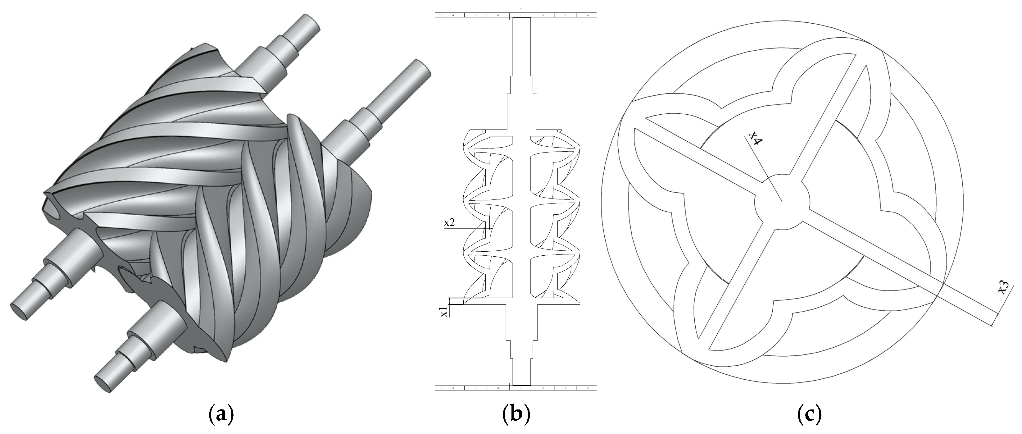
In the structural design modeling process, this study proposes a hollow internally supported screw rotor structure as shown in Figure 2. This proposal is based on the multi-physical field response characteristics of screw rotors under thermo–fluid–solid coupling loads and the forming ability of additive manufacturing processes for complex internal structures. By analyzing the structural redundancy of traditional solid rotors, it is found that the geometric parameters of the internal supporting structure significantly affect the rotor’s mass, stiffness, and modal characteristics. Therefore, this study uses key geometric parameters such as the supporting frame configuration and shell thickness as design variables for structural modeling and subsequent optimization, providing a structural basis for the green and lightweight design of screw rotors.
Guided by engineering practice and the requirements of automated simulation modeling, the design variable space was maximized. Following systematic parameter-sensitivity analysis and feasibility checks, four variables were defined: the thickness of the two end faces (X1), the thickness of the working gear face (X2), the width of the internal support rod (X3), and the diameter of the internal support column (X4). All four parameters lie within the rotor’s internal support structure, permitting lightweighting and stiffness enhancement without altering the external profile. The bounds are X1 ∈ [5, 35] mm, X2 ∈ [4, 40] mm, X3 ∈ [4, 16] mm, and X4 ∈ [20, 78] mm, as summarized in Table 2.
The choice of these independent parameters reflects their decoupling effect on multi-objective responses. X1 and X2 primarily govern the mechanical properties in the axial and meshing directions, respectively, whereas X3 and X4 cooperate to regulate radial support; together, they influence mass-distribution uniformity and dynamic stability. Outer-shape parameters (e.g., total rotor length and helix angle) are excluded because (1) the study targets hollow, internally supported rotors under a fixed outer contour, with optimization restricted to the internal structure; (2) the external profile is prescribed by a given profile equation and is not redesigned herein; (3) modifying the outer contour would necessitate rebuilding the coupled flow–thermal–structure models, substantially increasing computational cost and workflow complexity; and (4) any change in outer shape would trigger redesign of the casing and machine-level assembly, markedly increasing engineering effort. Concentrating on X1–X4 meets practical engineering constraints, preserves assembly compatibility, and achieves improvements in mass, stiffness, and dynamic performance through internal-structure optimization.

2.2.2. Multi-Physical Field Coupling Mechanism and Theoretical Characterization of Performance Indicators

To enable large-sample parametric simulations within a finite computational budget, a steady-state, one-way coupling workflow was adopted: a steady RANS flow solution provides the pressure distribution on the rotor surfaces; a steady thermal analysis yields the temperature field; both fields are then mapped to a static structural model to obtain the displacement and stress fields, from which the maximum total deformation (U) is extracted.
  • Multi-physical Field Coupling Mechanism: Fluid–structure interaction: The aerodynamic load on the rotor surface induces dynamic deformation. Thermo-structural coupling effect: The steady-state temperature gradient causes thermal stress, which combines with mechanical loads to form a composite stress field. Mass–dynamics correlation: Changes in mass distribution directly affect structural stiffness and modal characteristics.
  • Definitions of Key Performance Indicators: Maximum total deformation (U): Indicates the reduction in overall stiffness under thermomechanical loads. Mass (M): Reflects the lightweighting effect, calculated as the product of geometric topological volume and material density. First-order natural frequency (F1): Represents dynamic stability. A larger F1 reduces resonance risk by increasing the gap between the natural frequency and the operational base frequency.
  • Necessity of Surrogate Models: The aforementioned indicators exhibit strong nonlinear coupling, and the high-dimensional design space renders analytical solutions impractical. To address this, parametric simulations are used to generate high-dimensional datasets, and surrogate models are constructed to facilitate efficient multi-objective optimization. Implementation details regarding the platform (ANSYS 2022R1), material (316L stainless steel), and boundary conditions are provided in Section 3.2.

2.2.3. Acquisition of Sample Dataset

In this study, all design variables are sampled within preset continuous intervals. To uniformly cover the design space and enhance sample representativeness, a training dataset is generated using Latin Hypercube Sampling (LHS). Compared to simple random sampling, LHS can significantly reduce prediction variance with the same sample size. It is especially suitable for the high-dimensional, nonlinear coupled simulation models in this study. Balancing surrogate model complexity and computational cost, 180 samples were generated. Table 3 presents a representative subset of the data used in this study.

2.3. SNRBO Algorithm

2.3.1. Fundamentals and Procedure of the NRBO Algorithm

Algorithm Overview: NRBO is a population-based metaheuristic algorithm. It combines the Newton–Raphson method’s gradient-driven local search with the global search of population-based approaches. This enables it to efficiently solve complex continuous optimization problems. The algorithm has two key mechanisms: the Newton–Raphson Search Rule (NRSR) and the Trap Avoidance Operator (TAO). NRSR uses gradient-based local search, while TAO helps escape local optima. Together, they dynamically balance global exploration and local exploitation, improving convergence speed and solution accuracy.
  • Algorithm Initialization:
Let the objective function be f(x), where x R d is the d-dimensional design variable vector, and the variable bounds are defined as lb and ub. Initialize the population X = x 1 , x 2 , , x N , with individuals generated using the following formula:
x n = l b + r a n d × u b l b , n = 1 , 2 , , N
where N is the population size.
2.
Newton–Raphson Search Rule (NRSR):
In NRBO, the NRSR operator mimics Newton’s method by using second-order gradients. It constructs differential approximations to update positions, with the core formula as follows:
x n n e w = x n r a n d n × X w X b × x 2 × X w + X b 2 x n
The NRSR operator in NRBO mimics Newton’s method’s second-order gradient idea. It constructs a differential approximation to update the position. The core formula is as follows:
x = r a n d 1 , d X b x n t
To further enhance the exploitation ability, a guide term ρ is introduced. The specific formula is as follows:
ρ = a X b x n t + b X r 1 X r 2
Finally, the updated individual’s position is:
x n n e w = x n N R S R + ρ
Here, randn denotes a normal distribution random number, and a , b 0 , 1 . Xr1 and Xr2 are two individuals randomly selected from the population. This method uses differences to approximate first- and second-order derivatives, eliminating the need for explicit gradient information and thus is suitable for non-smooth objective functions.
3.
Trap Avoidance Operator (TAO):
It incorporates population mean information and disturbance factors to assist individuals in escaping local optima and constructing new solutions. The specific calculation formula is as follows:
X TAO = X u p d a t e + θ 1 ( u 1 X b u 2 X i ) + θ 2 δ ( u 1 X ¯ u 2 X i ) , u 1 < 0.5 X b + θ 1 ( u 1 X b u 2 X i ) + θ 2 δ ( u 1 X ¯ u 2 X i ) , o t h e r w i s e
In Formula (6), Xupdate is the candidate solution obtained after the basic iterative update. θ 1 1 , 1 , θ 2 0.5 , 0.5 are random disturbance factors that balance exploration and exploitation. X ¯ is the population mean, reflecting the central tendency of the population. u1 and u2 are self-adaptive parameters that dynamically adjust the reliance on the global optimum and the individual’s current state during new solution construction. They are defined as follows:
u 1 = β 3 r a n d + ( 1 β ) , β ( 0 , 1 ) 1 , o t h e r w i s e u 2 = β r a n d + ( 1 β ) , β ( 0 , 1 ) 1 , o t h e r w i s e
In Formula (7), β ( 0 , 1 ) serves as a binary disturbance switch. If r a n d < D F , then XTAO replaces the original individual.
4.
Update and Iteration Control:
In each iteration, new solutions are generated by NRSR and TAO. If a new solution has a better fitness value than the original individual, it replaces the original one. If the termination condition (reaching the maximum number of iterations T m a x ) is met, the iteration stops and the optimal solution X b is output.
NRBO combines Newton’s method’s local search with population-based optimization’s global exploration. It constructs two core operators, NRSR and TAO, to achieve efficient exploration–exploitation balance. The algorithm dynamically adjusts search strategies via adaptive parameters, making it suitable for high-dimensional, multimodal, constrained optimization problems. It has shown excellent performance in engineering design, wireless communication, and other fields. Its key advantages are being gradient-free and having low computational complexity. It can escape local optima effectively, providing a robust solution for complex optimization problems.

2.3.2. Design of the SNRBO Algorithm

While NRBO performs well in continuous optimization with good convergence and local exploitation, it faces challenges in high-dimensional nonlinear problems and complex search spaces. Specifically, the original algorithm lacks flexibility in search disturbance control, population structure regulation, and behavioral guidance. This makes it hard to adapt to different optimization stages, causing premature convergence or unstable convergence in multi-peak environments.
To further enhance the algorithm’s search stability, ability to escape local optima, and adaptive regulation levels, this paper proposes an improved algorithm called SNRBO, which integrates multiple strategies into the original NRBO framework. The algorithm integrates six intelligent mechanisms: attention mechanism, dynamic disturbance factor regulation, Lévy flight disturbance, hierarchical population updating, memory repository guidance, and genetic algorithm co-evolution. Through organic integration and collaborative interaction of these strategies, SNRBO conducts more adaptive and robust searches of the optimization space. It provides a solution framework with greater exploration depth and exploitation precision for complex optimization problems.
  • Dimensional Attention Mechanism:
To adaptively adjust variable-dimension importance and enhance the optimization process’s directionality and efficiency, this study integrates a dimensional attention mechanism into the SNRBO algorithm. In high-dimensional optimization, variables differ in sensitivity to the objective function. Traditional equal-weight update strategies fail to identify key variables, reducing optimization efficiency and causing local optima. The dimensional attention mechanism measures the activity of each dimension in the current population using its standard deviation, assigning differential search weights to different dimensions. The formula is as follows:
w j = σ j k = 1 d σ k , j = 1 , 2 , , d
In Formula (8), σ j denotes the standard deviation of the population on the j-th dimension, and d is the number of variable dimensions. A higher weight indicates greater dimension volatility and a more significant impact on the objective function. The individual update formula with the weight incorporated is as follows:
X update j = w j a 1 a 1 X 1 j + 1 a 2 X 2 j + 1 a 2 X 3 j
In Formula (9), a 1 , a 2 0 , 1 , and X1, X2, X3 are candidate solutions in the search process. This approach enables the algorithm to focus on dimensions with greater impact on the optimization objective, improving search efficiency and optimization accuracy.
2.
Adaptive Regulation Mechanism of Dynamic Disturbance Triggering Factor DF:
In the original NRBO algorithm, the disturbance probability DF used to trigger TAO perturbations is fixed, making it unable to adapt to the dynamic disturbance intensity requirements of different search stages. SNRBO introduces an adaptive disturbance probability regulation strategy based on the Sigmoid function, enabling the DF value to dynamically adjust with the iteration process. The specific expression is as follows:
D F = D F max D F max D F min 1 + e x p γ t t 0
In Formula (10), DFmin = 0.1, DFmax = 0.9, t0 = 0.7 Tmax and γ = 0.025 . Here, Tmax represents the maximum number of iterations. If the random disturbance probability condition is met, the trap avoidance operation is activated, and the specific operation is consistent with Formula (6) in Strategy 3.
3.
Lévy Flight Strategy:
To enhance the global search ability of SNRBO and address the insufficient global search capability of traditional NRBO, Lévy flight strategy is incorporated into SNRBO. This strategy increases the leap-like and discontinuous characteristics in individual search behavior. The Lévy flight strategy incorporated into SNRBO generates step-length distributions with heavy-tailed characteristics. This allows individuals to balance fine-tuning in short-distance movements with long-distance jumps, improving the algorithm’s ability to escape local optima. The Lévy distribution is constructed as follows:
L e v y ψ = u v 1 / ψ , u ~ N 0 , σ u 2 , v ~ N 0 , σ v 2
In Formula (11), u and v are random variables following a normal distribution, and ψ 1 , 2 , typically taken as 1.5, is the key parameter controlling the Lévy flight characteristics. Together, these elements determine the step length of the Lévy flight. The individual update formula under Lévy perturbation is as follows:
X n new = X n + 0.01 X n X b Levy ψ
In Formula (12), Xn is the position of the current individual within the population that requires an update. This strategy significantly improves individuals’ ability to jump. It expands the solution-space coverage and increases the chance of finding the global optimal solution in complex optimizations.
4.
Hierarchical Population Structure and Differential Behavior Strategy:
To enhance differentiated control and coordinated optimization of individual behaviors, a grouped-individual strategy is introduced into the SNRBO algorithm. In the original NRBO, all individuals are updated uniformly, lacking fitness-driven hierarchical optimization. This may destroy good solutions through perturbation and waste computational resources on poor individuals. In SNRBO, the population is divided into elite and exploration groups based on fitness ranking.
Elite Group: The top 20% of individuals by fitness are selected for local exploitation. Elite individuals indicate the current optimal solution direction. So, they undergo minor conservative-strategy perturbations to prevent damage to optimal information. In the later stages of SNRBO, elite individuals undergo small-magnitude perturbations based on the tangent distribution. The update formula is as follows:
X n new = X n + ϵ t a n π r 0.5 , ϵ = δ 1 it T max
In Formula (13), r ∈ (0, 1) is a random variable, and ϵ is the self-adaptive perturbation step-length, which gradually decreases with iterations. This strategy improves the local exploitation of elite solutions, maintaining the stability of the optimal structure while exploring neighboring solutions. The elite group adopts a very low disturbance probability, as shown in formula:
D F e l i t e = 0.3   ×   D F
This setting significantly reduces the risk of destroying high-quality solutions. The initial disturbance probability is capped at 0.27, protecting promising solutions found in the early exploration phase. In later stages, the probability drops to a minimum of 0.03, ensuring stable convergence during the exploitation phase.
Exploration Group: The bottom 30% of individuals by fitness are selected for leap-like search operations to increase population search breadth. Individuals in the exploration group, having poor fitness and limited guidance value, adopt an aggressive global search strategy to expand the search boundaries. SNRBO introduces Levy flight perturbations to the exploration group. This enhances their ability to make leaps and bounds, preventing the population from falling into local optima. A dual-exploration safeguard mechanism is adopted. The Levy flight strategy serves as the primary perturbation mechanism, while the TAO perturbation acts as a supplementary one. Individuals in the exploration group first undergo a triggering determination for Levy flight perturbations. The triggering probability formula is as follows:
D F explore = 0.5 + 0.4 D F
Explorers not triggered for Levy flight are highly likely to undergo subsequent TAO perturbation, with the triggering probability formula as follows:
D F i = min D F 2 , 0.9
Regular Group: Ordinary individuals, neither elite nor explorers, update based on the adaptive disturbance factor DF. Their update integrates Newton-directed search and TAO perturbation, aligning with the NRBO algorithm’s calculation process in Section 2.3.1. This “robust exploitation and aggressive exploration” strategy enhances the overall search. The exploration group handles global tasks, the elite group focuses on local exploitation, and the Regular Group connects the two. This improves solution diversity and quality.
5.
Memory Repository Collaborative Fine-Tuning Mechanism:
The memory repository guidance mechanism aims to use historical elite solutions to reconstruct and repair underperforming individuals. This enhances the algorithm’s search stability and convergence accuracy. In the traditional NRBO algorithm, the utilization rate of elite solutions is low, making information disconnection and falling into local optimum more likely.
In SNRBO, a fixed-capacity memory repository is designed to record several current optimal solutions after each iteration. In subsequent iterations, an elite solution is randomly selected from the repository to perform a linear-combination update with the current worst-performing individual. The specific calculation formula is as follows:
X new = α X i + 1 α X mem , α 0.3 , 0.8
In the formula: X m e m is an elite solution randomly selected from the memory archive (the historical best solution). This mechanism effectively inherits outstanding genetic information, mitigates population degradation, and enhances the overall search ability of the population.
6.
GA-based Information Reconfiguration and Population Co-evolution Strategy:
The genetic algorithm-based co-evolution mechanism is introduced into SNRBO, aiming to enhance the population diversity and realize the information recombination. In traditional NRBO, the lack of genetic-based crossover and mutation operations between individuals during the update process can lead to premature convergence. To address this, a co-evolution mechanism is introduced. This mechanism consists of three steps: selection, crossover, and non-uniform mutation.
Crossover Operation: To achieve information recombination and enhance structural diversity among individuals, the genetic algorithm sub-module in SNRBO introduces a linear-combination-based crossover strategy. Suppose two parent individuals, Xparent1 and Xparent2, are selected from the current population. A new individual X child can be generated using the following formula:
X child = λ X parent 1 + 1 λ X parent 2 , λ 0 , 1
Here, λ is a randomly sampled weight parameter from a uniform distribution, which dictates the genetic contribution of each parent to the offspring. When λ = 0.5, the offspring is a blend of both parents with equal weights. In contrast, when λ approaches 0 or 1, the offspring closely resembles one parent more than the other. This crossover operation facilitates the generation of new solutions between existing ones, thereby enhancing the algorithm’s search ability and population diversity.
Non-uniform Mutation Operation: To enhance the search ability and fine-tuning capacity of individuals during evolution, the GA module in SNRBO introduces a non-uniform mutation mechanism. This strategy allows the mutation step-size to gradually decrease with the iteration progression, achieving a smooth transition from global search to local convergence. The mutation update form on the j-th dimension is as follows:
X j mut = X j + t , d j
Here, dj = Oj − Xj is an adaptive perturbation term related to the current iteration number. It is defined as follows:
t , d j = d j 1 z 1 t T m a x c
In this framework, z ∈ (0, 1) represents a random perturbation factor, t is the current iteration number, Tmax denotes the maximum number of iterations, c is a mutation decay control factor, and Oj indicates the upper bound of the j-th variable. The function is designed to ensure substantial perturbations in the early stages and a tendency towards zero in later stages. This allows mutation to exhibit jumping behavior in the initial phase and local convergence capability in the final phase. This strategy provides additional leap paths and novel gene combinations outside the primary search trajectory, thereby enhancing the algorithm’s global optimization capability and robustness while effectively mitigating premature convergence.
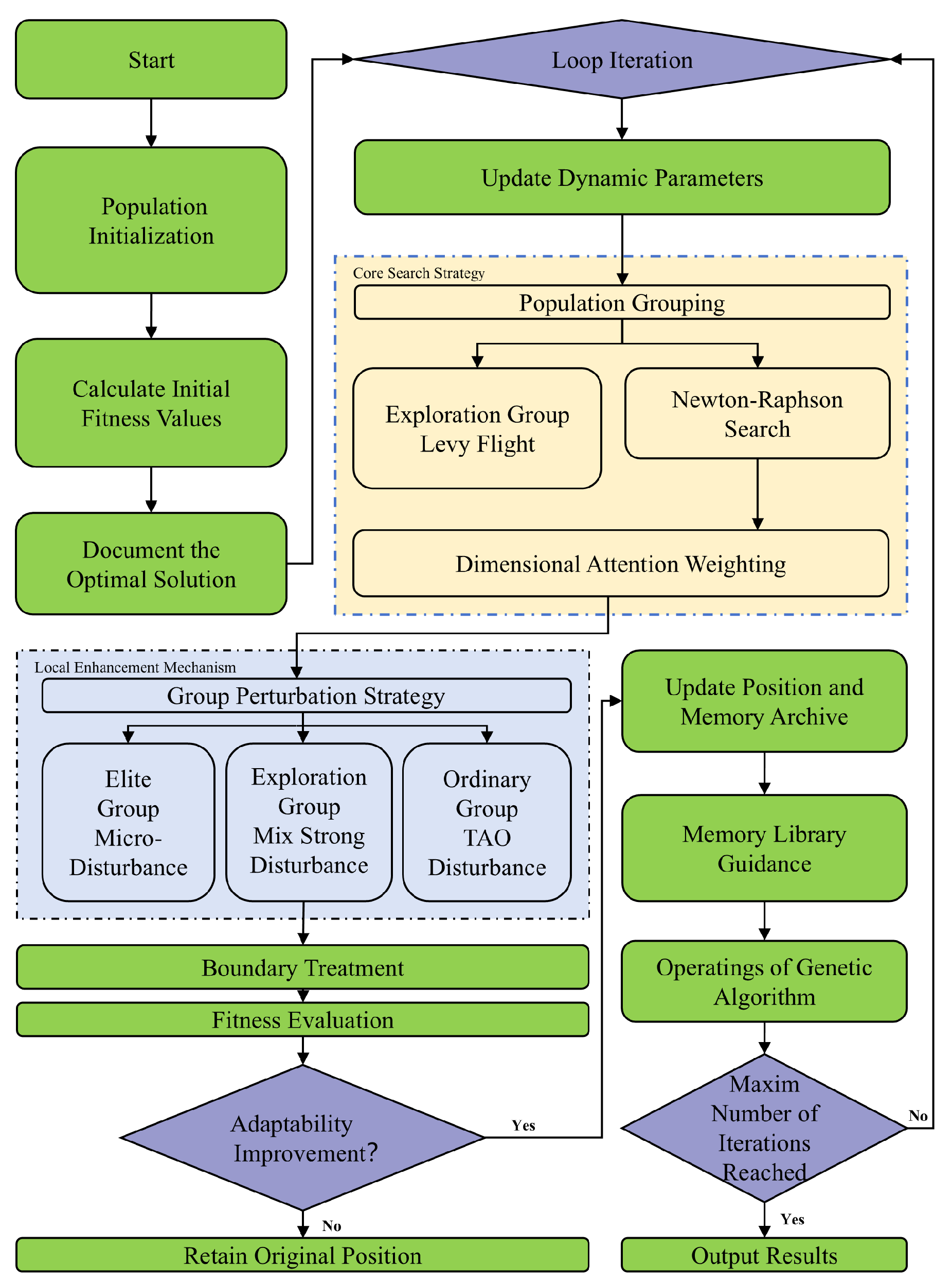
Figure 3 illustrates the flowchart of SNRBO, and the pseudocode describing the procedure from initialization to the final optimal solution is presented in Algorithm A1 in the Appendix A. The execution order within each iteration is as follows: Step 1—initialize the population and evaluate fitness to identify the current best solution Xb and open an empty memory archive; Step 2—update the iteration’s dynamic parameters, including the disturbance schedule and associated probabilities, then rank individuals and partition the population into elite, exploration, and regular groups; Step 3—promote global exploration by attempting Lévy-flight moves for the exploration group and accept an update when fitness improves; Step 4—for the remaining individuals, generate Newton-directed candidate solutions, apply dimensional-attention weighting, introduce adaptive perturbations according to group settings, enforce boundary conditions, and greedily accept improvements while updating Xb and the memory archive; Step 5—at scheduled intervals, repair the worst individuals using the memory repository and apply genetic operators—selection, crossover, and non-uniform mutation—to reconfigure information and sustain diversity; Step 6—in the late phase, apply small micro-perturbations to elites to refine local exploitation, then verify the stopping criterion and either proceed to the next iteration or report the best solution.

2.3.3. Design and Verification of Ablation Experiment

To reveal the marginal contribution of each enhancement, the ablation study adopts a progressive cumulative design. The baseline is NRBO. SNRBO1 augments NRBO with dimensional attention weighting. SNRBO2 further introduces adaptive regulation of the disturbance factor DF via a sigmoid schedule. SNRBO3 additionally incorporates a three-layer population mechanism with a dynamic Lévy-flight probability to strengthen global exploration. SNRBO4 adds a memory repository that guides the reconstruction of underperforming individuals using archived elites. SNRBO5 integrates GA-based co-evolution, including selection, crossover, and non-uniform mutation, together with a late-stage elite micro-perturbation to refine exploitation. All methods are evaluated under an identical protocol with 3000 iterations, a population size of 100, and a problem dimensionality of 30. The test functions are taken from the CEC2005 benchmark suite for single-objective real-parameter optimization, covering unimodal, multimodal, hybrid, and composition classes with shifted and rotated landscapes; the official problem definitions, search ranges, and evaluation criteria are followed [39]. Benchmark functions and their global optima are summarized in Table 4, and the comparative results from NRBO through SNRBO5 are reported in Table 5, with key data provided; the complete dataset is presented in Table A1 in Appendix A.
To assess the individual and synergistic effects of each strategy on the performance of the SNRBO algorithm, a comprehensive ablation study was conducted. The results demonstrate a clear trend of progressive performance enhancement as strategies are successively incorporated. Specifically, all versions from NRBO to SNRBO5 successfully converge to the theoretical optima on functions F1, F2, F3, F4, F9, and F11, with zero standard deviation, indicating high precision and robustness in these problems. In functions F8 and F14, intermediate versions (SNRBO1 to SNRBO4) exhibited some fluctuation in average performance compared to NRBO. Nevertheless, SNRBO5 achieved the best results, with F14 converging to −12,569.486, yielding a relative error of only 1.11 × 10⁻⁴, effectively reaching the theoretical optimum of −12,569.5.
For functions F5, F6, and F7, the average fitness progressively improved across all versions, with SNRBO5 reaching an exceptional convergence level on the order of 6.512 × 10⁻²³, reflecting a substantial improvement in precision. In functions F12, F13, and F15, while SNRBO1 achieved performance gains over NRBO, the introduction of the adaptive DF strategy in SNRBO2 led to slight degradation in average performance, possibly due to convergence instability without complementary mechanisms. However, when combined with the Lévy flight and hierarchical population strategies in SNRBO3, the average fitness dropped by four orders of magnitude, highlighting the effectiveness of their integration. Overall, the results verify that the proposed strategies, when applied in a staged manner—ranging from baseline enhancement, adaptive parameter control, exploration expansion, stability reinforcement, to global coordination—collectively enable the algorithm to achieve or approach theoretical optima in most benchmark functions. This demonstrates a well-balanced improvement across exploration depth, convergence accuracy, and algorithmic robustness.

2.3.4. Analysis of the Optimization Effects of Multi-Strategy Integration

To verify the improved effectiveness of the algorithm, performance was evaluated on the CEC2017 benchmark suite for single-objective bound-constrained real-parameter optimization [40]. The suite comprises F1 and F3 as unimodal functions (F2 was removed in CEC2017), F4–F10 as simple multimodal functions, F11–F20 as hybrid functions, and F21–F30 as composition functions (definitions and domains are listed in Table 6) [40]. All methods were run on the same platform under a common protocol: 3000 iterations, a population size of 100, and a problem dimensionality of 10. The compared algorithms included NRBO, SNRBO, the Dung Beetle Optimizer (DBO), the Grey Wolf Optimizer (GWO), and the Salp Swarm Algorithm (SSA), with parameter settings summarized in Table 7. For each function, the best value, mean, and standard deviation were recorded; best results are highlighted in bold, where the best value indicates optimization accuracy and the mean/standard deviation reflect stability.
The results of the experiments based on 29 benchmark functions are presented in Table 8, with key data provided. The complete dataset is available in Table A2 in the Appendix A. The SNRBO algorithm showed remarkable superiority in three metrics: min, std, and avg. When comparing SNRBO with the original NRBO algorithm, the results were as follows.
In terms of min: SNRBO secured 18 wins, 6 ties, and 5 losses. In terms of std: SNRBO achieved 22 wins and 7 losses. In terms of avg: SNRBO attained 28 wins and 1 loss. The comprehensive experimental results demonstrate that the improved SNRBO algorithm significantly outperforms the original NRBO in terms of convergence accuracy, stability, and overall optimization performance, thereby validating the effectiveness of the proposed enhancement strategies. Moreover, SNRBO achieves the best performance in terms of the average metric on 19 occasions when compared with the other four algorithms, further highlighting its robustness and stability across various problem scenarios.
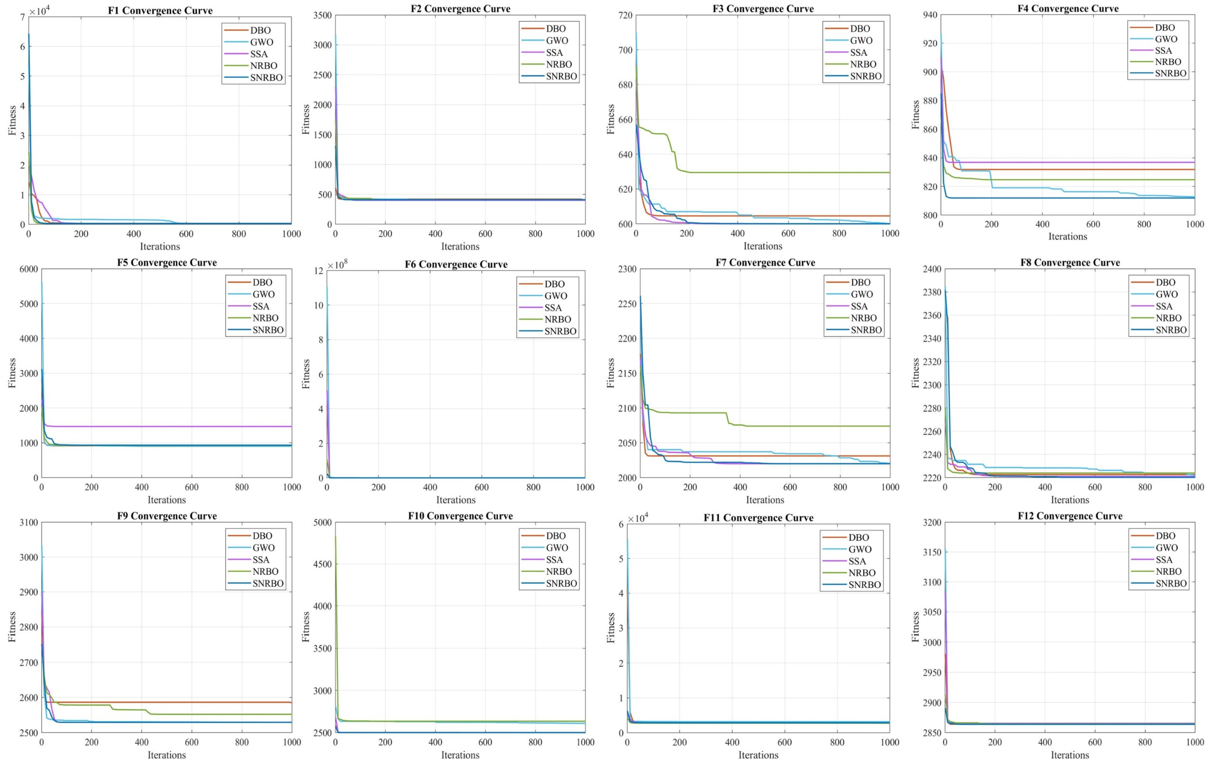
To further validate the convergence efficiency and robustness of the proposed SNRBO algorithm, comparative experiments were conducted on the CEC2022 benchmark function which covers diverse shifted/rotated hybrid and composition landscapes set (F1–F12) against DBO, GWO, SSA, and the original NRBO algorithms [41]. Figure 4 illustrates the convergence curves of all algorithms over 1000 iterations.
For unimodal functions such as F1 and F2, SNRBO (represented by the dark blue curve) exhibits a rapid decrease in fitness values during the early iterations and converges near the global optimum within fewer iterations. Compared to DBO, GWO, SSA, and the original NRBO, SNRBO achieves faster and more stable convergence, indicating its strong capability in solving smooth, single-peak problems with high local search efficiency.
In multimodal functions F3–F8, SNRBO maintains steep fitness descent and achieves lower final objective values on most test cases. Particularly, its convergence path in F3 is more compact, effectively avoiding premature convergence. The performance on F4–F8 further confirms its robustness in navigating complex multimodal landscapes and achieving a well-balanced trade-off between exploration and exploitation.
For hybrid and composite functions F9–F12, SNRBO continues to perform robustly. In F9 and F10, the convergence curves remain smooth and stable with lower fitness values, showcasing strong adaptability to irregular and multi-region search spaces. Although the final convergence values of most algorithms are comparable on F11 and F12, SNRBO’s optimization trajectory is more stable and continuous, emphasizing the effectiveness of its integrated attention mechanism and dynamic control strategies in complex search environments.
In summary, the convergence results on the CEC2022 benchmark set validate the superior performance of SNRBO in terms of convergence speed, stability, and accuracy across diverse optimization scenarios, highlighting its potential for real-world engineering applications.

2.4. Construction of SNRBO-Optimized XGBoost Surrogate Model

2.4.1. XGBoost Model

XGBoost, proposed by Chen and Guestrin [42], is a scalable tree-boosting method. It makes two core improvements upon GBDT. First, it adds a regularization term to the objective function. This constrains model complexity, preventing overfitting and enhancing generalization. Second, it uses a second-order Taylor expansion for the objective function, unlike GBDT’s first-order. This significantly boosts computational accuracy.
Model details are as follows: Let the dataset be D = x i , y i i = 1 , 2 , , n , where xi and yi represent the input features and target values, respectively. For a model trained with k trees, the predicted value y ^ i can be derived through the model structure. The calculation formula is as follows:
y ^ i = k = 1 K f k x i , f k F
The objective function to be optimized is given by the following formula:
O b j = i = 1 n L y i , y ^ i + Ω f j
Among them, i = 1 n L y i , y ^ i is the training loss function, Ω f j is the model complexity. The objective function of the t-th iteration is as follows:
O b j ( t ) = i = 1 n L y i , y i ( t 1 ) + f t ( x i ) + γ T + 1 2 λ j = 1 T ω j 2
In the formula, Ω f i = γ T + 1 2 λ j = 1 T ω j 2 . The objective function obtained via second-order Taylor expansion is as follows:
O b j i = i = 1 n g i ω q x i + 1 2 h i ω q 2 x i + γ T + 1 2 λ j = 1 T ω j 2
Among them:
g i = L ( y i , y ^ i ( t 1 ) ) y ^ i ( t 1 ) , h i = 2 L ( y i , y ^ i ( t 1 ) ) y ^ i ( t 1 ) 2
The objective function can be further simplified to obtain the final objective function as follows:
O b j i = T = 1 T l e a f g i a 1 + 1 2 l e a f h i + λ a i 2 + γ T
Also, like other machine learning models, the XGBoost model has various hyperparameters. Below is an introduction to the key hyperparameters that need optimization, as shown in Table 9.

2.4.2. Evaluation Metrics for Regression Models

To effectively evaluate regression model performance, this study uses R2 and RMSE. R2 measures how close actual and fitted values are; values closer to 1 indicate better fit. RMSE quantifies the deviation between predicted and actual values. Calculation formulas are as follows:
R 2 = 1 i = 1 n y ^ i y i 2 i = 1 n y i y ¯ 2
R M S E = i = 1 n y ^ i y i 2 n
In the formulas, y i is the true value, y ^ i is the predicted value, y ¯ is the mean of the true values, and n is the number of samples in training or testing.

2.5. NSGA-III-Based Multi-Objective Optimization

2.5.1. Objective Functions and Constraints

In multi-objective optimization, an objective function must be built for each goal. To quickly predict and optimize structural responses, this study uses the SNRBO-XGBoost model from Section 2.4 to model structural performance metrics. Specifically, it establishes a nonlinear link between key screw rotor parameters and performance responses via SNRBO-XGBoost. The model’s output serves as the objective function for optimization goals, expressed by the trained SNRBO-XGBoost predictor’s output function and integrated into the multi-objective optimization framework. The specific formula is as follows:
F X = min f m M X , U X , F 1 X
f m = S N R B O X G B o o s t x 1 , x 2 , x n
In the formula, fm denotes the output function for each optimization objective, and xn represents the set of variables to be optimized.
To obtain reasonable optimization results and avoid interference during model reconstruction of the hollow-supported screw rotor in each simulation, constraints are set for its structural parameters. These constraints are generally in the following form:
x m i n x i x m a x
In the formula, xi is the structural design parameter, while xmin and xmax represent the lower and upper bounds of the constraint, respectively.

2.5.2. NSGA-III Optimization Procedure

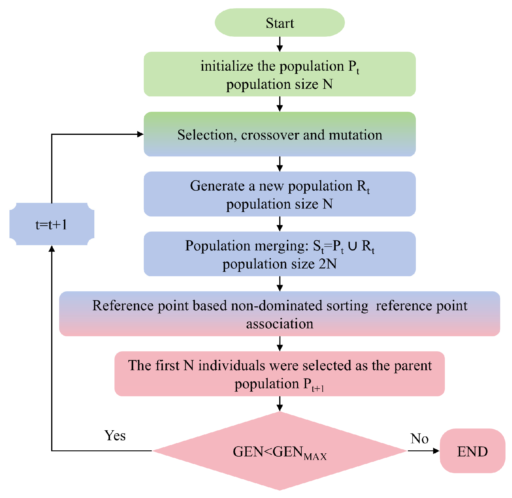
NSGA-III is applied to multi-objective optimization for reducing the mass and maximum total deformation of the hollow-supported screw rotor while increasing its first-order natural frequency. The NSGA-III-based workflow for constructing the Pareto frontier is illustrated in Figure 5.
After constructing the initial population P 0 of size N , uniformly distributed reference points Z r e f are generated (obtained by partitioning the hyperplane in the objective space, with a number matching the population size). Subsequently, non-dominated sorting is applied to P 0 to preliminarily classify individuals into different fitness levels, laying the foundation for subsequent genetic operations.
Based on the sorted initial population, the first-generation offspring population R 0 is generated using the three genetic mechanisms of GA (selection, crossover, and mutation).
In the second-generation evolution, the parent population P 0 and offspring population R 0 are merged into S 0 with a size of 2 N . Fast non-dominated sorting is applied to S 0 to obtain multiple non-dominated fronts. Subsequently, the objective space is normalized (by normalizing objective values based on the current population’s extremes). The Euclidean distance between individuals and reference points is calculated, associating individuals with reference points.
Based on the individuals’ non-dominated ranks and their association with reference points, environmental selection determines the new population P 1 . Starting from the highest rank, individuals are inductively included layer by layer until the population size approaches N . If the last layer cannot be fully selected, individuals associated with underrepresented reference points are prioritized to maintain population diversity.
Proceeding with population, repeat step 2.
Iterate steps 3–5 until the offspring reach the pre-set maximum generations. Finally, output the non-dominated front of the last-generation parent population as the approximate Pareto-optimal solutions.

2.5.3. Pareto Optimal Solutions

NSGA-III identifies a set of optimal solutions related to the Pareto-optimal state for multi-objective optimization problems. Like NSGA-II, it approximates the Pareto frontier rather than seeking a single optimal solution. In NSGA-III, reference points are introduced to guide population evolution. These points are predetermined in the objective space and help direct the optimization process.
NSGA-III first divides the population into different dominance levels. For each level, it selects individuals by calculating their association degree with each reference point. Suppose there are m objective functions f 1 x , f 2 x , , f m x . An individual x’s coordinates in the objective space are f 1 x , f 2 x , , f m x . The reference point r has coordinates r 1 , r 2 , , r m . The association degree D x , r is calculated as follows:
D ( x , r ) = i = 1 m f i ( x ) r i max j P   f i ( j ) min k P   f i ( k ) 2 1 / 2
Here, P denotes the current population. During selection, priority is given to individuals with a smaller association degree to reference points and those in higher-quality ranks. Through continuous iteration, the population gradually approaches the Pareto frontier. The solutions with the minimum association degree to reference points in the final set are the approximate Pareto-optimal solutions Uopt expressed as follows:
U opt = min D x , r r p
In this way, NSGA-III can effectively find the Pareto optimal solution set in multi-objective optimization problems, providing decision-makers with diverse and high-quality options.

3. Case Study on the Optimization of Hollow Internally Supported Screw Rotors

3.1. Case Description

The studied screw compressor, a specific industrial model, is used in a manufacturing plant’s compressed air supply system. The rated operating pressure of the screw compressor is 0.8 MPa, with a motor power of 30 kW. The baseline inlet air pressure is 0.1 MPa, the inlet temperature is 25 °C, and the outlet temperature is 50 °C. The screw compressor has a two-stage compression and air-cooled structure. Its core component, the screw rotor, uses a traditional solid design. However, this design’s redundancy leads to low material efficiency and high energy consumption, conflicting with green manufacturing goals. Lightweight design is needed to overcome these energy and material-utilization barriers. To meet the green manufacturing requirements of the “Made in China 2025” strategy and considering the recent rapid development of additive manufacturing technologies, this paper proposes a hollow internally supported rotor structure and a multi-objective optimization design method based on multi-physics coupling calculations and SNRBO-XGBoost-NSGA-III. The aim is to achieve a lightweight design for the screw rotor while enhancing its stiffness and dynamic response performance, thereby breaking through the technical bottlenecks of traditional solid screw rotors in terms of material utilization and processing energy consumption.

3.2. Rotor Structural Performance Simulation

3.2.1. Simulation Settings

After determining the design variables ( X 1 X 4 ) for the hollow-supported screw rotor in Section 2.2.1, this study established a parametric modeling environment on the ANSYS 2022R1 platform. It integrated static analysis, Fluent fluid solver, and steady-state heat conduction modules for multi-physics-field coupling simulation, aiming to accurately assess structural performance responses. Considering the rotor’s intended additive manufacturing, 316L stainless steel suitable for Selective Laser Melting (SLM) was chosen. Its physical and mechanical parameters are illustrated in Table 10.
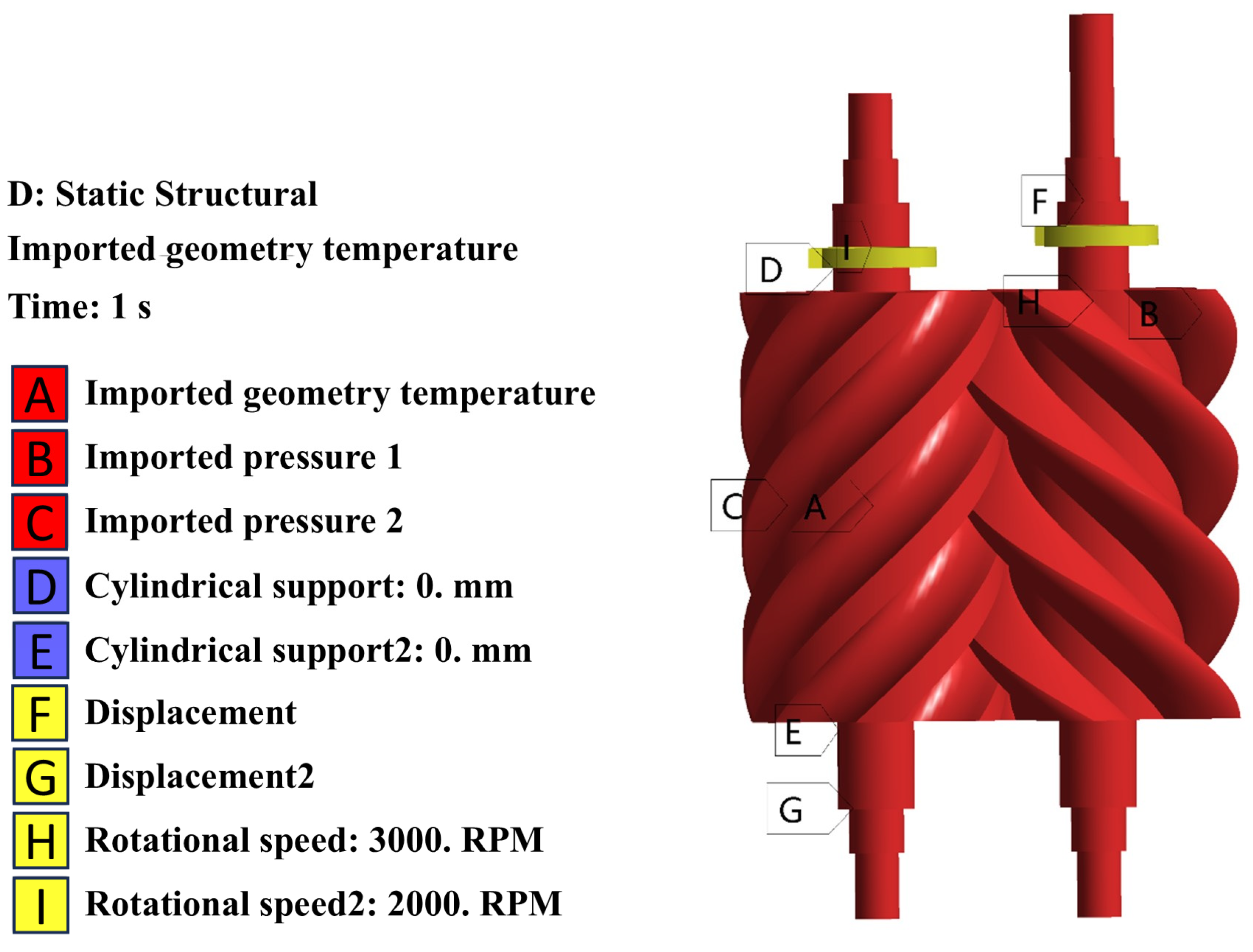
For a certain screw compressor model, the typical working condition is set with the male rotor speed at 3000 rpm and the female rotor speed at 2000 rpm. Based on the steady-state simulation of heat–flow–structure single-way coupling, the following key structural performance indicators are extracted:
Maximum total deformation (Y1): It evaluates the rotor’s stiffness under multi-physics-field coupling loads. The steady-state pressure distribution on the rotor surface (0.1–0.8 MPa) is obtained via the Fluent module, the temperature field distribution (inlet 25 °C, outlet 50 °C) is calculated by the steady-state heat module, and then the Static Structural module is used to perform structural static analysis to find the displacement extreme under the combined action of thermal expansion and fluid loads.
Mass (Y2): It reflects the structural lightweight level. The volume from the parametric model’s geometric features is automatically calculated and combined with the material density to get the structural mass data.
First-order natural frequency (Y3): Through the ANSYS Modal module, modal analysis is carried out. With the male rotor under fixed support boundary conditions, the first-order natural frequency is extracted to ensure it is away from the harmonic excitation range of the operating speed to avoid resonance.
The multi-physics coupling simulation process includes the following key steps: Fluid Pressure Field Calculation: Set the male rotor speed to 3000 rpm and the female rotor speed to 2000 rpm in the Fluent module, applying the Standard k-ε turbulence model and SIMPLEC method to compute the pressure load distribution on the rotor surface. Extract dynamic pressure contour plots from the meshing zone of the male and female rotors and export pressure load data to the Static Structural module for the working section of the screw rotor’s teeth.
Steady-State Temperature Field Analysis: Set the boundary conditions in the steady-state heat module with an inlet temperature of 25 °C and an outlet temperature of 50 °C. Apply a heat flux density of 17.3 W/mm2 on the meshing tooth surface of the screw rotor and take the convective heat transfer coefficient as 1.63 × 10⁻⁵ W/(mm2·°C). Solve for the internal temperature distribution of the rotor, generate the temperature gradient field, and export the temperature distribution data to the Static Structural module.
Pre-Stressed Modal Analysis: To evaluate the first-order natural frequency of the male rotor under actual assembly conditions, a prestressed modal analysis was conducted using the ANSYS Modal module by applying representative boundary constraints to simulate the preloaded state during assembly. The first six natural modes were extracted under prestress conditions, with a focus on the numerical value of the first-order natural frequency. This allows for assessing whether it remains sufficiently separated from potential external excitation frequencies, thereby providing a basis for evaluating the dynamic stability of the structure in service and offering a reference for ensuring frequency margin in subsequent design stages.
Thermal–Fluid–Structure Coupling Calculation: In multi-physics-field coupling simulations, the pressure distribution on the working-section tooth surfaces from fluid-field calculations is applied to the male and female rotors. The temperature distribution from steady-state thermal analysis is also imposed on the rotor structure to assess the combined effects of thermal–fluid–structure coupling on rotor performance. During compression in screw compressors, the radial force at the suction end is typically less than that at the discharge end. Proper bearing arrangement is crucial for enhancing structural stiffness and controlling deformation.
The model in this study uses a “fixed at one end and free to expand at the other” support condition, common in industrial assembly. Cylindrical roller bearings are located at the intake ends of the male and female rotors. These bearings prevent rotor tilting and radial motion but allow free rotation and axial movement. At the intake end, only rotation around the Z-axis and axial movement are allowed. At the exhaust end, cylindrical roller bearings are first used to handle radial loads and prevent tilting and radial motion. Then, four-point contact ball bearings are installed to take axial loads, restricting axial movement. This leaves only rotation around the Z-axis at the exhaust end, minimizing axial clearance to avoid end-face wear. The intake end retains larger axial clearance for thermal expansion. The specific load and constraint settings are illustrated in Figure 6.

3.2.2. Multi-Physics Coupling Analysis Results and Performance Extraction

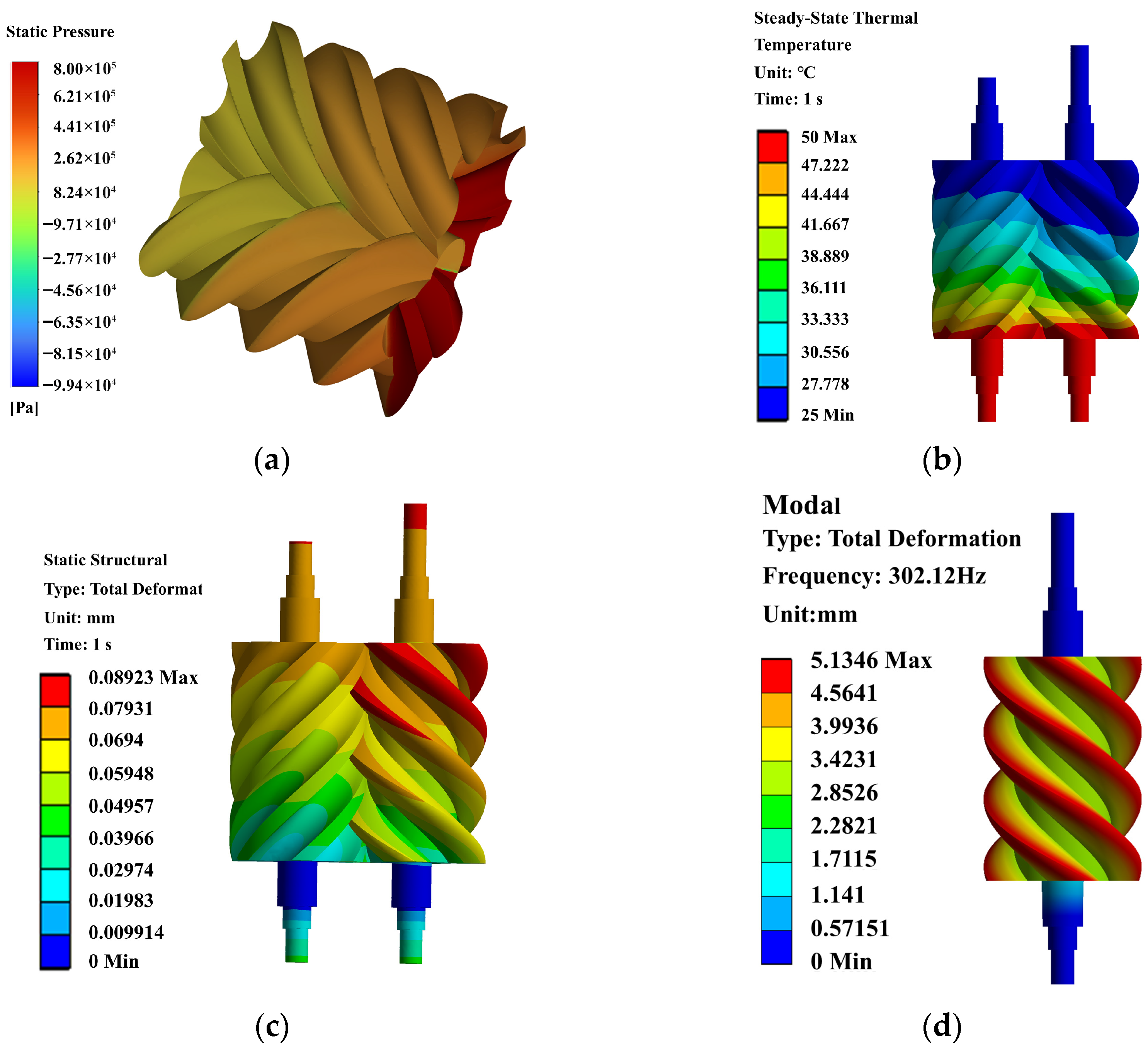
The simulation results for the original solid rotor model are illustrated in Figure 7, with a maximum total deformation (Y1) of 0.08923 mm, a mass (Y2) of 113.14 kg, and the first-order natural frequency (Y3) of 302.12 Hz.
Figure 7 presents the multi-physics-field coupling simulation results of a solid male rotor under typical working conditions, covering the fluid pressure field (Figure 7a), steady-state temperature field (Figure 7b), structural total deformation (Figure 7c), and modal analysis outcomes (Figure 7d). As observed, the rotor surface pressure primarily focuses between the middle of the compression section and the discharge end, ranging from 0.1 to 0.8 MPa. The temperature field exhibits a clear axial gradient, rising from 25 °C at the suction end to 50 °C at the discharge end.
In the static analysis, the maximum total deformation occurs at the top of the male rotor’s teeth at the suction end. This area, though subjected to relatively low load and temperature, is the free end with minimal bearing constraints. The thin-walled curved geometry here results in lower local stiffness, making it prone to deformation from stress release and thermal expansion. Additionally, fluid and thermal loads accumulate and propagate along the spiral path towards the suction end, amplifying displacement in this region.
The modal analysis in Figure 7d shows that the first-order natural frequency of the solid male rotor is higher than the harmonic excitation frequency range corresponding to the operating speed, ensuring a certain level of dynamic safety. However, this frequency is based on a heavy structure with redundant material and stiffness. If local stiffness is not properly maintained during lightweight design, the natural frequency may drop sharply, raising resonance risks. Thus, in subsequent optimization, it’s essential to enhance modal performance while reducing mass. This achieves a synergistic enhancement of mass and dynamic performance, ensuring high-speed operational stability.
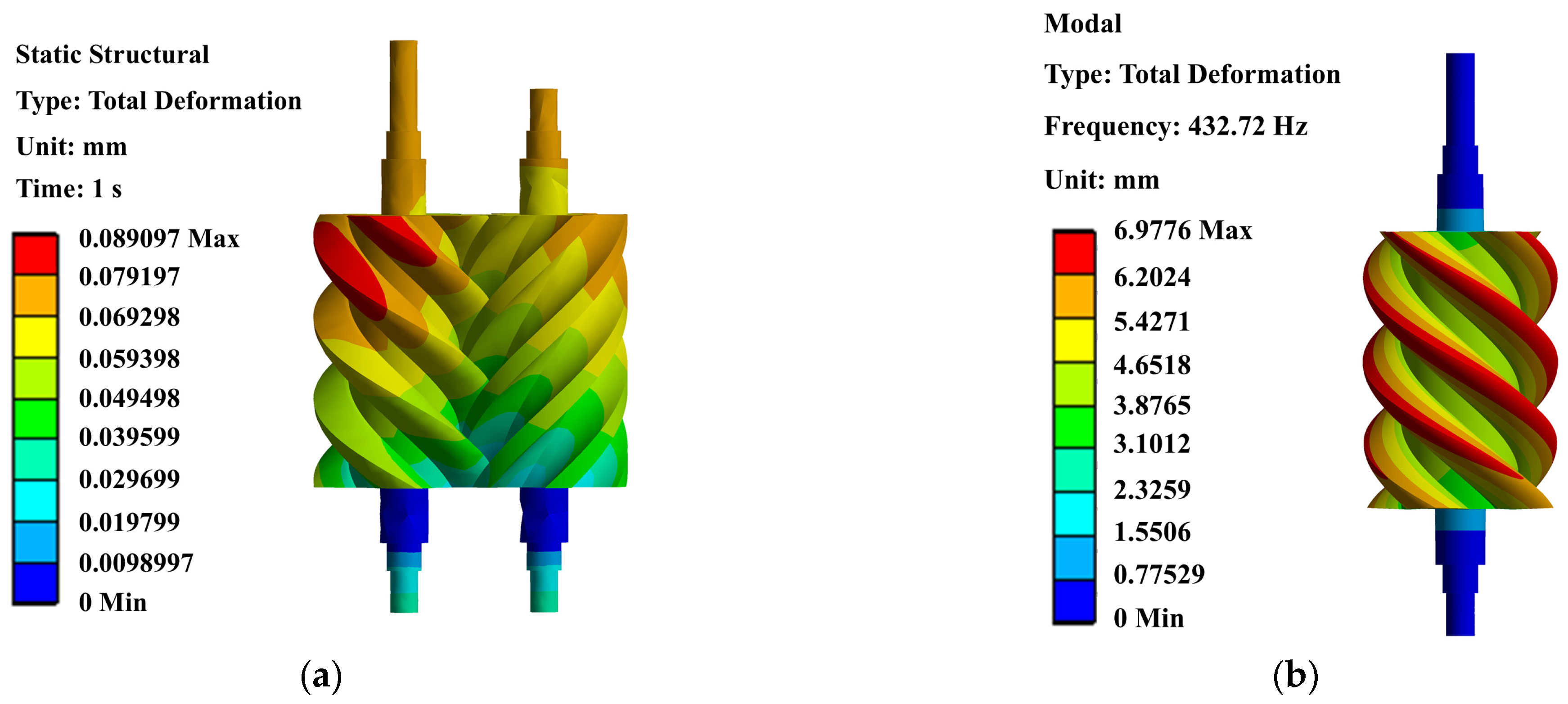
The sample results for [x1, x2, x3, x4] = [5.12, 10, 10, 77.8] are illustrated in Figure 8. For the lightweight model, the maximum total deformation (Y1) is 0.089097 mm, the mass (Y2) is 63.859 kg, and the first-order natural frequency (Y3) is 432.72 Hz.
Comparing the simulation results in Figure 7c,d shows that the optimized sample in Figure 8 significantly improves all performance metrics versus the original solid rotor. The maximum total deformation (Y1) decreases by approximately 0.15%, the mass (Y2) reduces by about 45.56%, and the first-order natural frequency (Y3) increases by roughly 43.70%. These results further confirm the effectiveness and feasibility of the proposed lightweight design method in enhancing rotor structural performance.
The above-mentioned indices are closely linked via multi-physics-field coupling. Fluid pressure and temperature fields jointly influence structural response, while mass distribution changes affect dynamic characteristics. This non-linear coupling relationship necessitates creating a high-fidelity surrogate model using precise simulation data to facilitate multi-objective optimization.

3.3. Performance Prediction and Validation Based on the SNRBO-XGBoost Model

3.3.1. Constructing XGBoost Prediction Model

Based on the 180 samples described in Section 3.2, this study developed a performance prediction model driven by XGBoost. The model takes four structural design variables as input features and predicts three optimization objectives: mass, maximum total deformation, and the first-order natural frequency. Prior to modeling, all data were normalized. For sample allocation, 70% of the data were randomly selected for model training, while the remaining 30% were used as a test set to validate the model’s predictive performance.
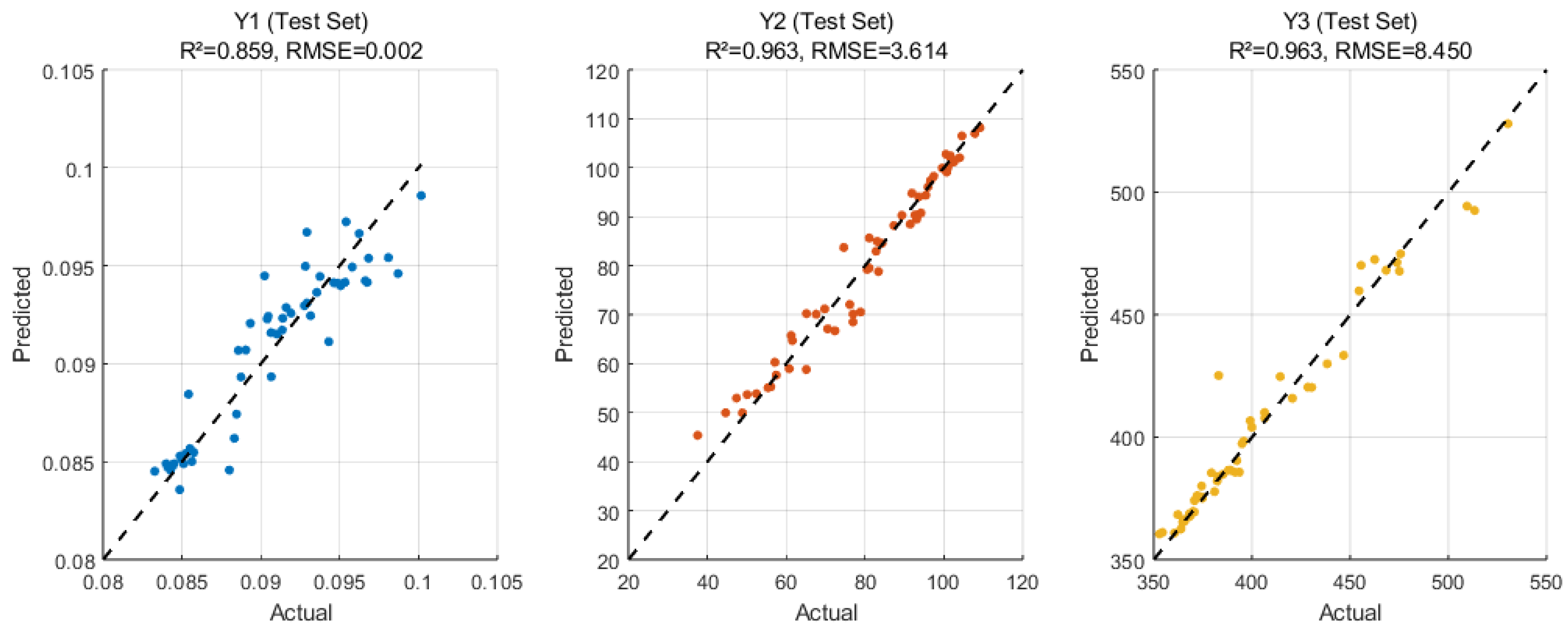
In this study, the hyperparameters in XGBoost were initialized as x = [num_trees (x1): 100, max_depth (x2): 7, eta (x3): 0.3]. The sample data were then input into the XGBoost model, and the model’s predictions are illustrated in Figure 9. The R2 and RMSE of the XGBoost model can be seen in the figure.
Under the default hyperparameter settings, the XGBoost model has certain predictive capabilities, but it has significant limitations in multi-output target scenarios. The test results indicate that for target Y1, the R2 is 0.859 and the RMSE is 0.002, indicating relatively poor performance and overfitting. However, for targets Y2 and Y3, the model performs well with an R2 of 0.963 and RMSE values of 3.614 and 8.450, respectively, showing strong fitting and generalization abilities.
These results suggest that the default hyperparameters struggle to balance the nonlinear relationships between multiple outputs, leaving room for optimization between fitting accuracy and generalization. Consequently, the next section introduces a hyperparameter optimization strategy based on the SNRBO algorithm. This approach aims to automatically adjust key XGBoost hyperparameters, such as the number of trees, maximum depth, and learning rate, to enhance the model’s overall predictive accuracy and robustness.

3.3.2. Hyperparameter Optimization of XGBoost Model Based on SNRBO

To obtain an XGBoost model with optimal hyper-parameters, the RMSE magnitudes of the three outputs Y1, Y2 and Y3 differ significantly; a direct arithmetic mean of the raw RMSE values would allow the indicator with the largest magnitude to dominate the objective function and eclipse the others. Consequently, each RMSE is first normalized to the interval [0,1], after which the normalized values are averaged to construct the objective function, expressed as follows:
F = R M S E Y 1 + R M S E Y 2 + R M S E Y 3 3
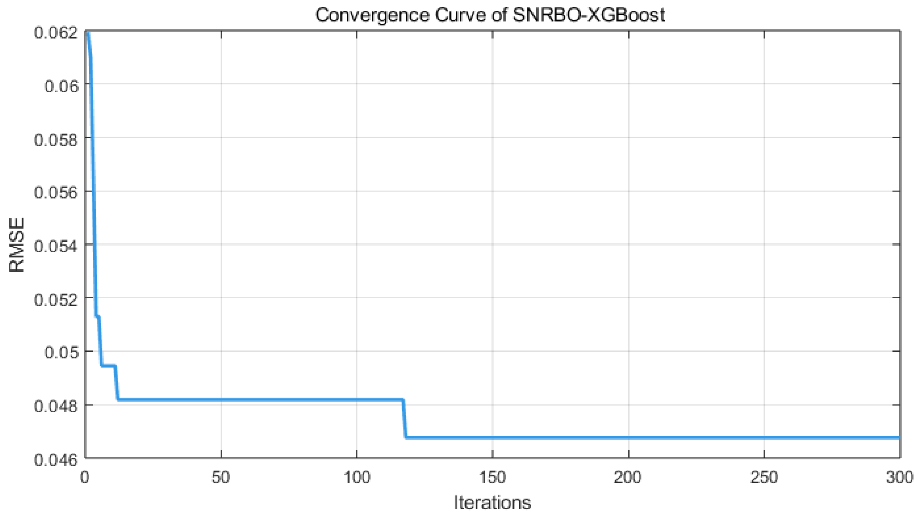
The optimal hyperparameter combination obtained is optimal in comprehensive performance for the three output variables, rather than being optimal for any specific output. The relationship between hyperparameters and the objective function is established using the SNRBO algorithm. Before this, the hyperparameter optimization space needs to be set, and the search is conducted within the hyperparameter space shown in Table 9. Then, the initial point is set to 50, and the number of iterations is set to 300, that is, p = 50 and n = 300. Through continuous iterative updates, a set of optimal hyperparameter combinations that minimize the objective function is found. The process of finding the optimal hyperparameter combination using the SNRBO algorithm is illustrated in Figure 10.
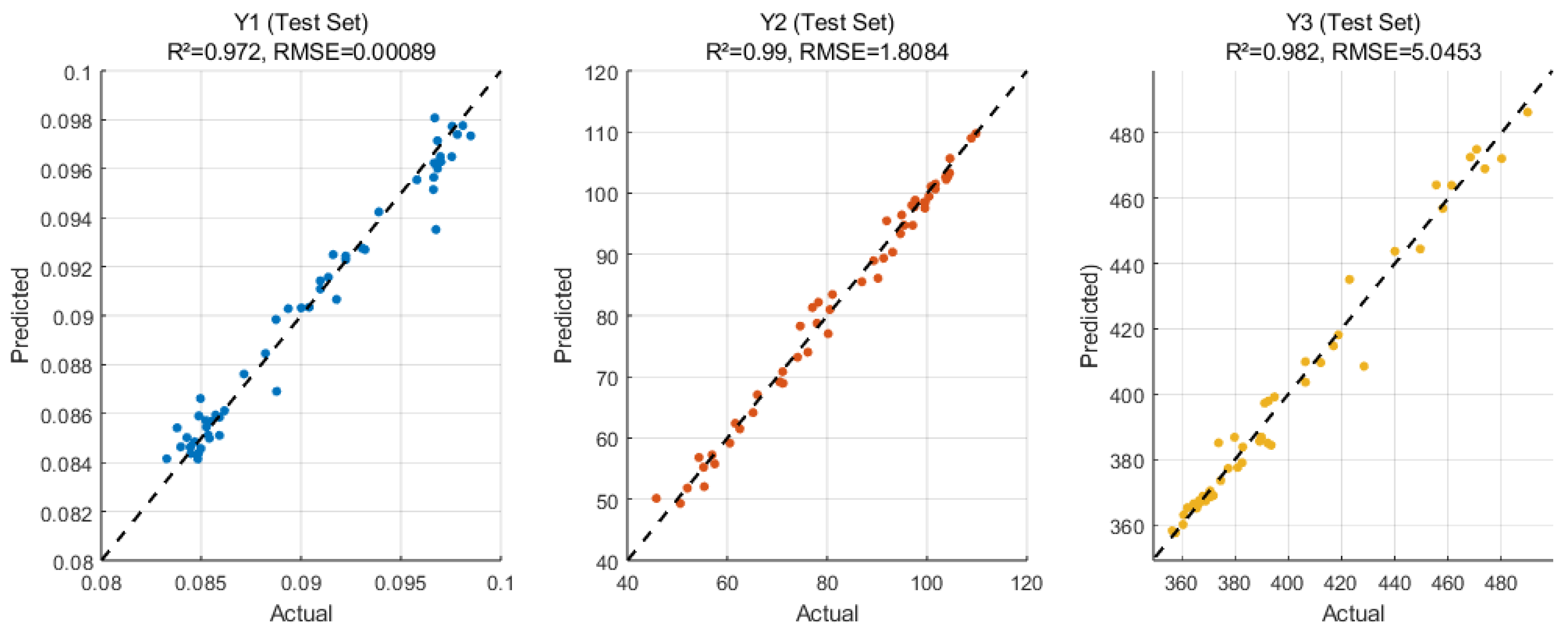
As the number of iterations increases, the program inputs hyperparameter combinations from the predefined hyperparameter space using the SNRBO algorithm. When N = 300, the iteration stops, and the model with the lowest RMSE value is output. After 300 iterative optimizations using the SNRBO algorithm, the optimal hyperparameter combination for comprehensive performance of the three output variables is obtained as x = [num_trees (x1): 252, max_depth (x2): 3, eta (x3): 0.0687]. The specific results on the test set are illustrated in Figure 11.
On the test set, the SNRBO-XGBoost model shows excellent predictive performance for the three output variables. Their R2 values are 0.972, 0.990, and 0.982, and the RMSE values are 0.00089, 1.8084, and 5.0453. These indicate high fitting accuracy and stability of the model. Compared to the default XGBoost model, the SNRBO-XGBoost model shows significant improvement in predictive accuracy:
  • Y1: R2 increases by 12.9%, RMSE decreases by 5.6%.
  • Y2: R2 increases by 2.8%, RMSE decreases by 49.96%.
  • Y3: R2 increases by 1.97%, RMSE decreases by 40.29%.
These results show that the SNRBO optimization strategy can effectively enhance the XGBoost model’s ability to fit complex nonlinear relationships between multiple objectives, improving its generalization performance.
In subsequent multi-objective optimization, the SNRBO-optimized XGBoost regression model is used as the fitness function. It can accurately reflect the mapping relationship between design variables and structural performance, providing a solid foundation for obtaining high-quality Pareto optimal sets and optimization solutions.

3.3.3. Multi-Objective Optimization of Hollow Internally Supported Screw Rotors Based on NSGA-III

In Section 3.3.2, SNRBO-XGBoost is used to establish a regression relationship between the objective function and design variables. This relationship serves as the fitness function in NSGA-III to assess the three-objective optimization problem of minimizing maximum total deformation, mass, and maximizing the first-order natural frequency without constraints, yielding a set of Pareto-optimal solutions.
Based on the ranges of the four design variables set in Section 2.2.1, this section aims to minimize the maximum total deformation Y1 and mass Y2 while maximizing the first-order natural frequency Y3.
The multi-objective optimization problem is defined as follows:
min f 1 ( S N R B O X G B o o s t ( X 1 , X 2 , X 3 , X 4 ) ) min f 2 ( S N R B O X G B o o s t ( X 1 , X 2 , X 3 , X 4 ) ) min f 3 ( S N R B O X G B o o s t ( X 1 , X 2 , X 3 , X 4 ) ) X 1 [ 5 , 35 ] X 2 [ 4 , 40 ] X 3 [ 4 , 16 ] X 4 [ 20 , 78 ]
In the formula, Y1 represents the maximum total deformation (U), Y2 represents the mass (M), and Y3 represents the first-order natural frequency (F1).
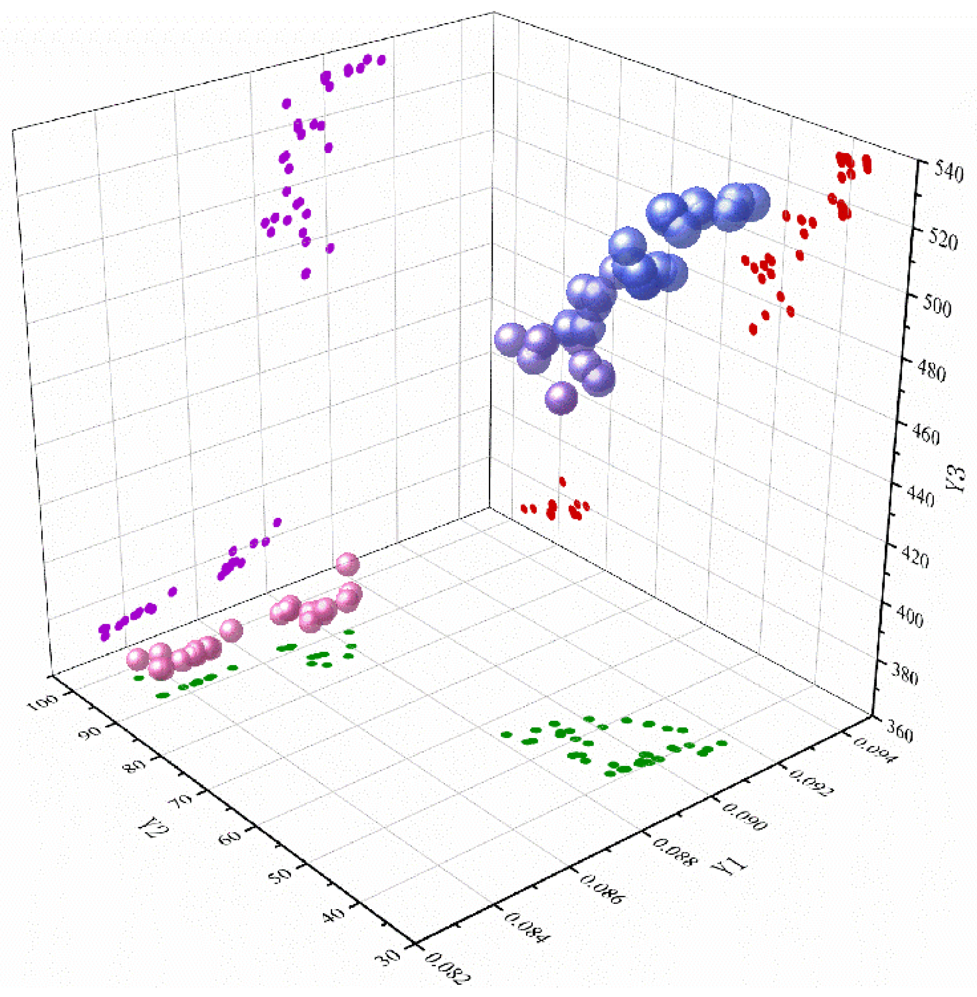
After defining the optimization problem, this study uses the MATLAB 2024 version to execute the SNRBO-XGBoost-NSGA-III framework program for screw rotor multi-objective optimization. Before conducting NSGA-III multi-objective optimization, it is essential to configure its parameters to balance Pareto front accuracy and computational efficiency. In this study, the population size is set to 50, the maximum number of iterations to 200, the crossover probability to 0.8, and the mutation probability to 0.05. Upon completion of the parameter settings, NSGA-III optimization was performed to generate the Pareto front, which is illustrated in Figure 12.
The primary objective of this study is the lightweight design of the screw rotor, for which a higher weight of 0.4 is assigned to mass to prioritize the reduction of material usage and the enhancement of energy efficiency. Meanwhile, to balance the rotor’s structural stability and dynamic performance, weights of 0.3 are assigned to deformation and first-order natural frequency, respectively. Controlling deformation and natural frequency is crucial for ensuring the stiffness of the structure and avoiding resonance. This weight distribution not only ensures the implementation of lightweight design but also balances the static and dynamic performance of the equipment, making it suitable for most engineering applications. Finally, the overall performance scores of the Pareto-optimal solutions are calculated, and the solution with the highest performance score is selected as the optimal solution. The design parameter values of this optimal solution are illustrated in Table 11.
The optimized lightweight screw rotor model is assigned material properties to obtain mass information. Coupled analysis and modal analysis are performed to get the maximum deformation, mass, and the first-order natural frequency of the optimized model. These values are compared with the pre-optimization values in Table 12 to check the feasibility of the optimization scheme for the screw rotor.
The performance parameters of the optimized screw rotor are compared with the original solid rotor in Table 12. During the multi-objective optimization, all design constraints are strictly met. The optimization results are significantly better than the original design. The maximum total deformation is reduced by 0.3%, the mass is reduced by 60.7%, and the first-order natural frequency is increased by 71.16%. These improvements are achieved while maintaining engagement accuracy and structural integrity, indicating remarkable enhancements in structural stiffness and dynamic performance.
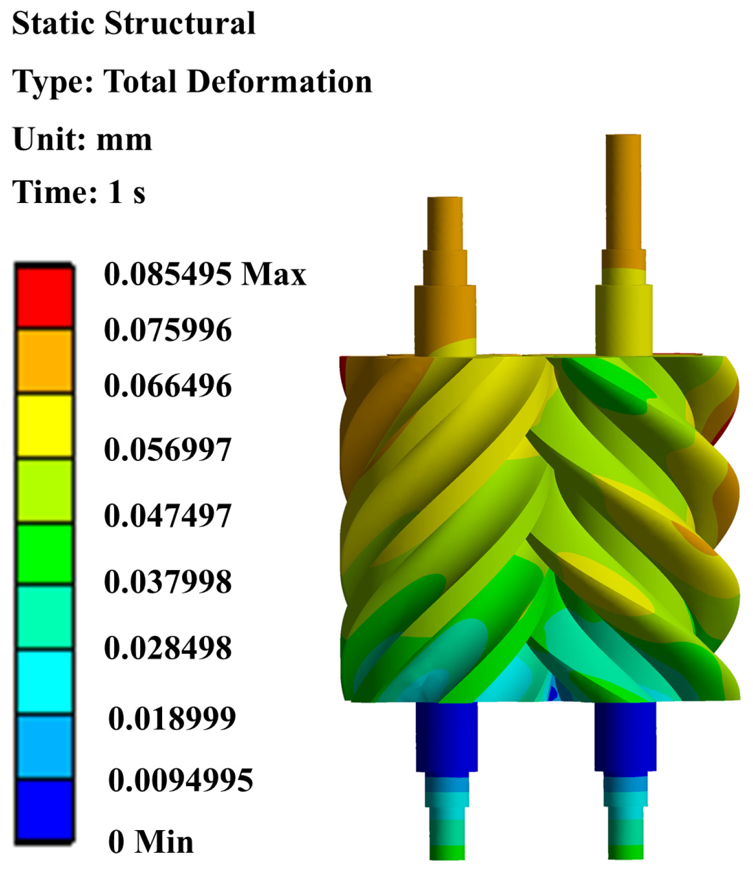
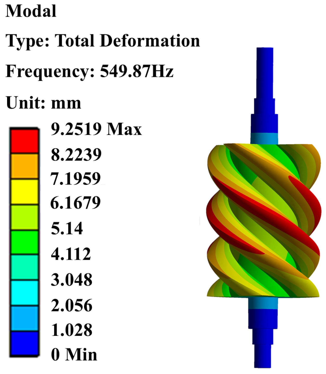
To verify the effectiveness of the optimized structure and the accuracy of the predictive model, further finite element simulation analysis was conducted on the optimized rotor, with results illustrated in Figure 13 and Figure 14. The simulation results for maximum total deformation, mass, and first-order natural frequency were 0.085495 mm, 40.38 kg, and 549.87 Hz, respectively. When compared to the predictions from the SNRBO-XGBoost model, the relative errors for these three indicators were 4.1%, 2.6%, and 4.1%, respectively. Compared to the initial solid screw rotor, the optimized hollow-supported screw rotor shows a 4.41% reduction in maximum total deformation, a 64.43% decrease in mass, and an 82.14% increase in first-order natural frequency. These results further confirm the high precision and good generalization capability of the predictive model in multi-physical-field response modeling.
In summary, the lightweight structural design and optimization method proposed in this paper not only achieves improvements in multiple performance objectives but also ensures the accuracy of structural response predictions and engineering feasibility. It provides an effective technical approach for the green and high-performance design of screw-rotor-type components.

4. Discussion

4.1. Limitations

Although the SNRBO-XGBoost-NSGA-III multi-objective optimization method works well in improving screw rotor structural performance and reducing weight, it has the following three limitations:

4.1.1. Additive Manufacturing Dependency

The hollow internally supported screw rotor design, with its complex internal features and asymmetric cavities, is currently manufacturable only via metal additive manufacturing. This limits its engineering applications and highlights unresolved issues in size control, residual stress, and surface quality during the additive manufacturing process.

4.1.2. Experimental Verification Is Restricted by Practical Operational Conditions

As the screw rotor rotates at high speed within the compressor’s confined space, it is currently difficult to deploy non-contact sensors or conduct online measurements to obtain real-time deformation and dynamic response data. Consequently, the structural optimization effects proposed in this paper mainly rely on simulation evaluation, lacking experimental validation. Future efforts should focus on indirect testing and sensor reconstruction to fill this validation gap.

4.1.3. The Optimization Objectives Have Not Covered All the Performance Requirements

The optimization model established in this paper uses maximum total deformation, mass, and first-order natural frequency as the main objective functions. These cover three key performance indicators: structural stiffness, lightweight design, and dynamic characteristics. However, it has not modeled or optimized other core indicators such as thermal stability, fatigue life, manufacturing cost, and noise during long-term operation. Therefore, the current optimization results cannot fully reflect the comprehensive performance of the structure over its entire life cycle.

4.2. Performance Comparison of Prediction Models

To verify the predictive performance of the proposed method in multi-objective regression modeling, this paper compares the SNRBO-XGBoost model with two common regression algorithms in machine learning: Kriging and Radial Basis Function (RBF) neural networks. All models are trained on an identical training set and assessed on an identical test set to guarantee the consistency and fairness of the comparison. The regression models are constructed using the MATLAB Regression Fitter module, with Kriging and RBF both using default hyperparameter configurations. The predictive performance of the three models on the test set is compared in Table 13, and fitting accuracy and generalization are evaluated using multiple metrics.
The experimental results show that the SNRBO-XGBoost model has the lowest RMSE and highest R2 for predicting maximum total deformation, mass, and first-order natural frequency. Its RMSE values are 0.0008, 1.8084, and 5.0453, and its R2 values are 0.978, 0.990, and 0.982, respectively. These results indicate that the SNRBO-XGBoost model has the highest fitting accuracy among the three models.

5. Conclusions

A lightweight screw-rotor design framework based on SNRBO–XGBoost–NSGA-III is presented, achieving joint optimization of mass, maximum total deformation, and first-order natural frequency. By balancing competing objectives, the method delivers a lighter rotor with improved structural stability and dynamic safety. Benchmark results show reduced mass alongside simultaneous gains in both static and dynamic performance.
These outcomes demonstrate strong potential to support engineering deployment of multi-objective rotor design and represent an effective solution for lightweighting under coupled performance constraints. The integration of data-driven surrogates with evolutionary multi-objective optimization provides reliable decision guidance across wide design ranges while maintaining modeling rigor.
Looking ahead, the framework will be extended to include outer-contour dimensions to increase design flexibility and overall performance; computational efficiency and scalability will be strengthened through parallelization and algorithmic acceleration; the objective set will be broadened to incorporate thermal stability, fatigue life, and operational noise; and uncertainty modeling with multi-condition response analysis will be integrated to enhance adaptability and robustness for green, efficient design of complex rotor structures.

Author Contributions

J.S.: Writing—original draft and Formal analysis; J.Z.: Methodology and Supervision; B.Z.: Data curation; H.Z.: Resources and Investigation; Y.Z.: Writing—review & editing; J.W.: Visualization. All authors have read and agreed to the published version of the manuscript.

Funding

This research was supported by the Joint Funds of the Zhejiang Provincial Natural Science Foundation of China under Grant No. LZY24E050003, as well as the Central Government’s Guidance Fund for Local Science and Technology Development, Project No. 2025ZY01027, for the construction of the Provincial Key Laboratory for Intelligent Manufacturing of Aerodynamic Equipment. Additionally, it was supported by the Zhejiang Key Laboratory of Intelligent Manufacturing for Aerodynamic Equipment under Grant No. 2025E10033.

Data Availability Statement

The data underlying this article will be shared on reasonable request to the corresponding author. Due to an ongoing patent application related to the core technology described in this manuscript, the full raw dataset cannot be made publicly available at this stage. Upon reasonable request, and subject to a Data Use Agreement (DUA) and institutional approval where applicable, the de-identified minimal reproducible dataset and analysis scripts can be obtained from the corresponding author (email: zjqaydf@163.com); requests will normally be answered within 5 working days.

Acknowledgments

The authors would like to express their gratitude to the Joint Fund of Zhejiang Provincial Natural Science Foundation for the financial support provided for this project.

Conflicts of Interest

Hehuai Zhu was employed by the company Zhejiang Chentai Machinery Manufacturing Co. The remaining authors declare that the research was conducted in the absence of any commercial or financial relationships that could be construed as a potential conflict of interest.

Abbreviations

The following abbreviations are used in this manuscript:
SNRBOenhanced Newton–Raphson-based optimization algorithm
NRBONewton–Raphson-based optimization algorithm
XGBoostextreme gradient boosting regression model
SHAPSHapley Additive exPlanations
NSGA-Ⅲnon-dominated sorting genetic algorithm III
NSGA-IInon-dominated sorting genetic algorithm II
R2Coefficient of determination
RMSERoot Mean Square Error
BOBayesian Optimization
SMOTESynthetic Minority Over-sampling Technique
RSMResponse Surface Methodology
GAGenetic Algorithm
FEFinite Element
RVEAReference Vector Guided Evolutionary Algorithm
HHOHarris Hawks Optimization
CNNConvolutional Neural Network
LSSVMLeast Squares Support Vector Machine
DBODung Beetle Optimizer
GWOGrey Wolf Optimizer
SSASalp Swarm Algorithm

Appendix A

Algorithm A1 SNRBO Algorithm Pseudo-Code
Input: N, T, DFmin, DFmax, γ, t0
Output: Xb, f(Xb),
1: Initialize population, evaluate fitness
2: Xb = best solution, M = empty set
3: for t = 1 to T do
4:   DF = DFmin + (DFmax − DFmin)/(1 + exp(γ(t − t0)))
5:   δ = (1 − 2t/T)^5, p_levy = 0.5 + 0.4*DF
6:   Rank population, divide into elite E and exploration P groups
7:   for each Xi in P do
8:     if rand < p_levy then
9:       Xi = Levy-Flight (Xi, Xb)
10:       Update if improved
11:     end
12:   for i = 1 to N do
13:     if (Xi in P and rand < p_levy) then continue
14:     ρ = rand*(Xb − Xi) + rand*(Xr1 − Xr2)
15:     X1 = Xi − α*NRSR + ρ, X2 = Xb − α*NRSR + ρ
16:     att_weights = normalized dimension variances
17:     Xupdate = attention_weighted_combination(X1, X2, att_weights)
18:     if Xi in E then DFi = 0.3*DF
19:     else if Xi in P then DFi = min(2*DF, 0.95)
20:     else DFi = DF
21:     if rand < DFi then
22:       Xnew = TAO_operator(Xupdate, Xb, mean(X))
23:     else
24:       Xnew = Xupdate
25:       if t > 0.3T and rand < 0.4 then
26:         Xnew = tangent_perturbation(Xnew)
27:       end
28:     if f(Xnew) < f(Xi) then
29:       Xi = Xnew, update Xb and M
30:     end
31:   if t > 0.4T and mod(t,5) = 0 then
32:      replace_worst_solution(M)
33:   end if
34:   apply_GA_operations()
35:   if t > 0.7T then perturb_elite(E)
36: end for
37: return Xb, f(Xb)
Table A1. Ablation Study Results: Optimization Performance of NRBO–SNRBO5 on CEC2005.
Fun.IndicatorNRBOSNRBO1SNRBO2SNRBO3SNRBO4SNRBO5
F1min000000
avg000000
std000000
F2min000000
avg000000
std000000
F3min000000
avg000000
std000000
F4min000000
avg000000
std000000
F5min25.713727.852728.444721.472421.76899.7922
avg28.877128.585128.336122.633922.196312.7850
std1.05290.29990.16100.96060.64511.4854
F6min1.64941.46001.13861.815 × 10−51.836 × 10−56.512 × 10−23
avg2.33342.21991.52241.432 × 10−41.949 × 10−45.138 × 10−18
std0.74180.65440.51551.629 × 10−42.679 × 10−41.178 × 10−17
F7min5.654 × 10−62.522 × 10−71.074 × 10−76.652 × 10−75.367 × 10−71.882 × 10⁻⁷
avg1.688 × 10−54.191 × 10−63.691 × 10−63.478 × 10−62.504 × 10−62.431 × 10⁻⁶
std9.616 × 10−63.304 × 10−63.551 × 10−62.922 × 10−62.421 × 10−62.253 × 10⁻⁶
F8min−12,568.9012,550.975−12,358.18−12,214.164−12,451.031−12,569.486
avg−11,973.12−11,157.92−11,003.45−11,714.179−11,784.138−11,977.295
std617.53751372.64291072.1951434.0522521.7963611.6129
F9min000000
avg000000
std000000
F10min4.441 × 10−164.441 × 10−164.441 × 10−164.441 × 10−164.441 × 10−164.441 × 10⁻¹⁶
avg4.441 × 10−164.441 × 10−164.441 × 10−164.441 × 10−164.441 × 10−164.441 × 10⁻¹⁶
std000000
F11min000000
avg000000
std000000
F12min0.092330.030570.0193062.273 × 10−65.987 × 10−76.572 × 10−24
avg0.1531020.0568470.0322476.185 × 10−64.492 × 10−61.234 × 10−18
std0.0547650.0253490.0227364.491 × 10−63.871 × 10−63.489 × 10−18
F13min1.1896160.7586490.9415980.0221440.0113234.351 × 10−23
avg1.6733661.1447472.028541.0546520.4282571.829 × 10−9
std0.4971720.2263360.7398451.1408540.4495705.783 × 10−9
F14min0.9980040.9980040.9980040.9980040.9980040.998004
avg0.9980041.1964141.1968091.1964141.3948240.998004
std00.6274280.4191190.6274280.8365710
F15min0.0003070.0003070.0003070.0003070.0003070.000307
avg0.0005820.0005820.0024450.0003070.0004100.000307
std0.0004420.0004420.0043101.7332 × 10−190.0002882.0284 × 10−19
F16min−1.03163−1.031628−1.031628−1.031628−1.031628−1.031628
avg−1.031629−1.031629−1.031629−1.031629−1.031629−1.031629
std1.282 × 10−167.402 × 10−171.047 × 10−1607.402 × 10−177.402 × 10⁻¹⁷
F17min0.3978870.3978870.3978870.3978870.3978870.397887
avg0.3978870.3978870.3978870.3978870.3978870.397887
std000002.5173 × 10−12
F18min333333
avg333333
std7.972 × 10−163.310 × 10−161.412 × 10−1501.099 × 10−157.402 × 10⁻¹⁶
F19min−3.862782−3.862782−3.862782−3.862782−3.862782−3.862782
avg−3.862782−3.862782−3.862782−3.862782−3.862782−3.862782
std9.004 × 10−169.362 × 10−169.004 × 10−169.362 × 10−169.004 × 10−169.362 × 10⁻¹⁶
F20min−3.321995−3.321995−3.321995−3.321995−3.321995−3.321995
avg−3.250659−3.274431−3.274434−3.262549−3.2744379−3.278761
std0.0613960.0613960.0614020.0626620.0613960.057431
F21min−10.15311−10.15311−10.15311−10.15311−10.15311−10.15311
avg−10.15311−10.15311−10.15311−10.15311−10.15311−10.15311
std1.184 × 10−151.324 × 10−151.675 × 10−151.324 × 10−151.026 × 10−155.921 × 10⁻¹⁶
F22min−10.40294−10.40294−10.40294−10.40294−10.40294−10.40294
avg−10.40294−10.40294−10.40294−10.40294−10.40294−10.40294
std1.872 × 10−151.324 × 10−151.184 × 10−151.675 × 10−151.184 × 10−152.581 × 10⁻¹⁵
F23min−10.53641−10.53641−10.53641−10.53641−10.53641−10.53641
avg−10.53641−10.53641−10.53641−10.53641−10.53641−10.53641
std1.450 × 10−151.450 × 10−151.324 × 10−151.675 × 10−152.777 × 10−151.776 × 10⁻¹⁵
Table A2. Statistical Results of Optimization Algorithms on the CEC2017 Benchmark Functions.
Fun.IndicatorSNRBONRBOSSAGWODBO
F1min100124,176.0025100817.51846173.12119
F1std336.4485452,396,364.033556.141662,984,131.26394475.46590
F1avg186.2792533,293,989.093337.874114,147,219.25995858.13815
F3min300313.9677300300.13304300
F3std091.0480601071.638550
F3avg300475.57855300852.53363300
F4min400402.19641400.00000403.14014400.07016
F4std031.14973015.4314213.38114
F4avg400430.56487400.3674412.35204406.94101
F5min504.9748516.57792503.97984504.05717504.97479
F5std8.843299.9696511.484165.954476.66001
F5avg518.97102533.57897525.30341511.03369522.70239
F6min600607.12295600.00000600.00891600.00000
F6std0.002067.804631.595850.355552.27558
F6avg600.00152619.90204601.10083600.15725602.33398
F7min713.91117730.24737731.59653712.33565708.97840
F7std7.2185121.0716123.754717.649137.46474
F7avg726.19065758.93307783.39142722.16173725.91688
F8min806.96471813.43160812.93446807.97522808.95463
F8std6.403878.969278.988233.174688.82478
F8avg818.34038827.06885823.92535809.62024822.93602
F9min900.00000905.84990900.00000900.01313900.00000
F9std5.6544767.08529354.265172.820683.68053
F9avg905.42374984.950431145.74665901.14792901.29885
F10min1133.812421421.277551280.611801015.425571147.38275
F10std270.04951250.57236240.40111251.58968253.89499
F10avg1711.609062006.604091683.821571400.527671606.67873
F11min1101.989921119.557901102.985241102.951271104.97934
F11std11.5112140.1005725.7305011.7325129.66915
F11avg1119.062041166.711621128.692441117.483811132.33242
F12min1451.385902897.217611982.239616897.366082508.87278
F12std2694.8359610,265.7773415,364.86967328,359.16152,110,737.0396
F12avg4216.8918314,370.9659815,577.15813177,246.949070,3962.56377
F13min1302.984141405.036861327.097642022.790461443.23262
F13std12.583601982.949615687.097234092.652205864.18388
F13avg1316.876562504.879806217.545358182.660885145.97250
F14min1406.967741440.783681420.973551434.100571422.13311
F14std14.3860835.9366546.26779931.8876338.43662
F14avg1430.251071495.492761478.918791709.673691469.24885
F15min1501.023711533.721431505.591841502.625781503.52932
F15std4.8012175.0664157.04805889.74214113.36744
F15avg1506.693201635.575941557.517091913.939491635.95996
F16min1600.229311605.902061601.209171608.013911601.65460
F16std102.02903131.97874111.2692875.5071177.53228
F16avg1693.029661748.418291742.961381689.352981686.18223
F17min1700.331901730.066911704.301921721.335171716.85587
F17std21.3837230.7367751.7966632.9460115.16309
F17avg1725.702951769.444331769.238661746.260281739.29766
F18min1800.512911838.392421826.822002255.440641838.56018
F18std196.365081867.813893151.6095513687.3660716810.86183
F18avg1897.600932360.410534057.2380328533.3289116812.07757
F19min1900.027371911.920551903.431851909.464301902.56311
F19std1.3135263.1101753.677613485.08861173.65993
F19avg1901.748501973.057501957.932043062.914612002.41438
F20min20002055.745242004.604182020.109182000.62435
F20std9.6560050.8626847.5510835.3154242.25531
F20avg2016.354792129.973552054.976152045.314732052.15641
F21min22002202.672302200.000002200.908342200.00000
F21std63.0898666.7004363.2242241.315471.49200
F21avg2281.363012270.732462301.773452293.256952203.48697
F22min2217.520842250.914512235.398252215.190462237.05251
F22std17.7451114.7676020.0419517.6270420.43483
F22avg2301.399412320.006992302.312162302.582022297.86689
F23min2610.698612610.803792607.447242600.002722613.17756
F23std12.9277213.1929412.366206.7673510.01144
F23avg2632.233102633.039742635.556922611.951982626.76312
F24min25002512.014832742.200242512.707082500.00000
F24std70.6264276.9625416.2171242.94487132.10737
F24avg2749.043792738.780772769.674512732.946292631.45750
F25min2897.837532900.377862600.118832897.978382897.99141
F25std37.2532127.2209864.2986618.7909124.45282
F25avg2937.278962939.775352916.723632925.107832933.46772
F26min26002776.192162815.562542900.032022900.00000
F26std250.89507233.66277346.84593185.6898053.65751
F26avg3023.639743069.355433164.224782942.262373016.90388
F27min3092.519523091.434323089.308083089.518193089.54597
F27std29.5231219.5743511.3529216.153902.94698
F27avg3112.322353100.394653099.400173096.151723095.25721
F28min3100.000003135.703473100.000003100.053923100.00000
F28std148.53881124.59793133.97350112.45144120.61598
F28avg3339.642323339.142283312.586793335.651323280.41282
F29min3159.134113159.770303130.644203132.323373133.24937
F29std51.4265360.4093570.0430327.5634165.29587
F29avg3231.410203228.671913253.312663162.528713222.27078
F30min3461.498453957.632633875.685955716.629503861.09668
F30std490,258.8057471,382.8663383,885.7759640,575.4247347,806.93168
F30avg333,555.0316396,657.6868210,909.85553518,213.5952241,165.22062

References

  1. Ulu, E.; Huang, R.; Kara, L.B.; Whitefoot, K.S. Concurrent Structure and Process Optimization for Minimum Cost Metal Additive Manufacturing. ASME J. Mech. Des. 2019, 141, 061701. [Google Scholar] [CrossRef]
  2. Li, Y.; Zhao, X.; Liu, S.; Wang, C.; Shen, S.; Guo, Y. Review and Prospects of Numerical Simulation Research on Internal Flow and Performance Optimization of Twin-Screw Compressors. Energies 2025, 18, 2608. [Google Scholar] [CrossRef]
  3. Aydın, A.; Engin, T.; Kovacevic, A. Design optimisation of a screw compressor with a focus on rotor depth: A computational fluid dynamics approach. Int. J. Refrig. 2025, 170, 385–397. [Google Scholar] [CrossRef]
  4. Dhayanandh, K.K.; Rameshkumar, K.; Sumesh, A.; Lakshmanan, N. Influence of oil injection parameters on the performance of diesel powered screw air compressor for water well application. Measurement 2019, 152, 107323. [Google Scholar] [CrossRef]
  5. Kaufmann, F.; Irrgang, L.; Schifflechner, C.; Spliethoff, H. Fast and accurate modelling of twin-screw compressors: A generalised low-order approach. Appl. Therm. Eng. 2024, 257, 124238. [Google Scholar] [CrossRef]
  6. Zhao, B.; Chen, H.; Gao, D.; Xu, L.; Zhang, Y. Heat transfer simulation in cavity of twin screw compressor under coupling of clearance leakage-heat by utilizing fuzzy beamlet finite element model. J. Therm. Anal. Calorim. 2021, 143, 3221–3232. [Google Scholar] [CrossRef]
  7. Tian, Z.Y.; Zhao, Y.Q.; Li, Z.H.; Liu, S.; Wang, D.H. Optimization and characteristic analysis of screw rotor of a twin-screw pump. J. Vibroeng. 2023, 25, 171–188. [Google Scholar] [CrossRef]
  8. Deng, Z.; Chen, Q.; Zhang, L.; Fu, Z. Data driven NARMAX modeling for PEMFC air compressor. Int. J. Hydrogen Energy 2019, 45, 20321–20328. [Google Scholar] [CrossRef]
  9. Kumar, A.; Patil, S.; Kovacevic, A.; Ponnusami, S.A. Performance prediction and Bayesian optimization of screw compressors using Gaussian Process Regression. Eng. Appl. Artif. Intell. 2024, 133, 108270. [Google Scholar] [CrossRef]
  10. Wang, T.; Qi, Q.; Zhang, W.; Zhan, D. Research on Optimization of Profile Parameters in Screw Compressor Based on BP Neural Network and Genetic Algorithm. Energies 2023, 16, 3632. [Google Scholar] [CrossRef]
  11. Tran, V.Q.; Wu, Y.R. Uniform-design-based multi-objective optimization for twin-screw rotor profiles generated by sealing line. Mech. Mach. Theory 2025, 209, 105985. [Google Scholar] [CrossRef]
  12. Saravana, A.; Liu, H.; Able, N.; Collins, J.; Groll, E.A.; Ziviani, D. Conjugate heat transfer analysis of a twin-screw compressor with 4–6 configuration and internal cooling channels. In IOP Conference Series: Materials Science and Engineering; IOP Publishing: Bristol, UK, 2022; Volume 1267, p. 012014. [Google Scholar] [CrossRef]
  13. Zhang, Y.; Huan, C.; Chao, R.; Wan, Z.; Zhi, M.; Wan, X. Design and Analysis of New Screw Rotor Structure Based on the 3D Printing Technology. Mech. Res. Appl. 2020, 33, 19–22. [Google Scholar] [CrossRef]
  14. Chao, R. Research on Structural Design and Processing Method of Hollow Screw Rotor. Master’s Thesis, Shanxi University of Technology, Shanxi, China, 2021. [Google Scholar] [CrossRef]
  15. Wan, Z. Design and Optimization of Lightweight Screw Rotor with Hollow Inner Support. Master’s Thesis, Shanxi University of Technology, Shanxi, China, 2021. [Google Scholar] [CrossRef]
  16. Zh, M. Research on Lightweight Design and Additive Manufacturing Technology of Screw Rotor of Air Compressor. Master’s Thesis, Shanxi University of Technology, Shanxi, China, 2022. [Google Scholar] [CrossRef]
  17. Bandini, A.; Cascino, A.; Meli, E.; Pinelli, L.; Marconcini, M. Improving Aeromechanical Performance of Compressor Rotor Blisk with Topology Optimization. Energies 2024, 17, 1883. [Google Scholar] [CrossRef]
  18. Wu, C.; Pan, H.; Luo, Z.; Liu, C.; Huang, H. Multi-objective optimization of residential building energy consumption, daylighting, and thermal comfort based on BO-XGBoost-NSGA-II. Build. Environ. 2024, 254, 111386. [Google Scholar] [CrossRef]
  19. Liu, Z.; Cui, Z.; Wang, M.; Liu, B.; Tian, W. A machine learning proxy based multi-objective optimization method for low-carbon hydrogen production. J. Clean. Prod. 2024, 445, 141377. [Google Scholar] [CrossRef]
  20. Han, Y.; Wei, Z.; Huang, G. An imbalance data quality monitoring based on SMOTE-XGBOOST supported by edge computing. Sci. Rep. 2024, 14, 10151. [Google Scholar] [CrossRef] [PubMed]
  21. Mao, F.; Chen, M.; Zhong, K.; Zeng, J.; Liang, Z. An XGBoost-assisted evolutionary algorithm for expensive multiobjective optimization problems. Inf. Sci. 2024, 666, 120449. [Google Scholar] [CrossRef]
  22. Mehdary, A.; Chehri, A.; Jakimi, A.; Saadane, R. Hyperparameter optimization with genetic algorithms and XGBoost: A step forward in smart grid fraud detection. Sensors 2024, 24, 1230. [Google Scholar] [CrossRef] [PubMed]
  23. Fu, J.; Wang, H.; Sun, X.; Bao, H.; Wang, X.; Liu, J. Multi-objective optimization for impeller structure parameters of fuel cell air compressor using linear-based boosting model and reference vector guided evolutionary algorithm. Appl. Energy 2024, 363, 123057. [Google Scholar] [CrossRef]
  24. Zivkovic, M.; Tair, M.; Bacanin, N.; Hubálovský, Š.; Trojovský, P. Novel hybrid firefly algorithm: An application to enhance XGBoost tuning for intrusion detection classification. PeerJ Comput. Sci. 2022, 8, e956. [Google Scholar] [CrossRef]
  25. Huang, M.; Zhao, H.; Chen, Y. Research on SAR image quality evaluation method based on improved harris hawk optimization algorithm and XGBoost. Sci. Rep. 2024, 14, 28364. [Google Scholar] [CrossRef]
  26. Lima Marinho, T.; do Nascimento, D.C.; Pimentel, B.A. Optimization on selecting XGBoost hyperparameters using meta-learning. Expert Syst. 2024, 41, e13611. [Google Scholar] [CrossRef]
  27. Li, Q.; Chu, W.; Ji, T.; Wang, H.; Guo, Z. SHAP-XGBoost Enabled Aerodynamic-Structural Balance in Transonic Compressors: T-shaped Groove Casing Treatment Design with Data-Driven Parameter Decoupling. Aerosp. Sci. Technol. 2025, 164, 110391. [Google Scholar] [CrossRef]
  28. Wang, J.; Chen, B.; Wang, Y.; Pu, D.; Jia, X. Research on four-bar linkage trajectory synthesis using extreme gradient boosting and genetic algorithm. J. Comput. Des. Eng. 2024, 11, 1–21. [Google Scholar] [CrossRef]
  29. Sowmya, R.; Premkumar, M.; Jangir, P. Newton-Raphson-based optimizer: A new population-based metaheuristic algorithm for continuous optimization problems. Eng. Appl. Artif. Intell. 2023, 128, 107532. [Google Scholar] [CrossRef]
  30. Huan, B.; Li, X.; Wang, J.; Hu, T.; Tao, Z. An interpretable deep learning model for the accurate prediction of mean fragmentation size in blasting operations. Sci. Rep. 2025, 15, 11515. [Google Scholar] [CrossRef]
  31. Li, Z.; Wang, M.; Xu, R.; Jiang, J.; Li, J.; Zhang, Z.; Yang, A. Prediction of viscosity of blast furnace slag based on NRBO-DNN model. Alex. Eng. J. 2025, 119, 124–137. [Google Scholar] [CrossRef]
  32. Li, Y.; Ni, L.; Chen, G.; Zhang, L.; Yao, N.; Wang, G. Neuro-enhanced fractional hysteresis modeling and identification by modified Newton-Raphson optimizer. Appl. Math. Model. 2025, 140, 115865. [Google Scholar] [CrossRef]
  33. AbouOmar, M.S.; Eltayeb, A.; Al-Quraishi, M.S.; El Ferik, S. Parameter Estimation of Proton Exchange Membrane Fuel Cells Using Chaotic Newton-Raphson-Based Optimizer. Results Eng. 2024, 24, 103369. [Google Scholar] [CrossRef]
  34. Shi, W.; Liang, Q.; Sun, L. Path Planning for Yarn Changing Robots Based on NRBO and Dynamic Obstacle Avoidance Strategy. Appl. Sci. 2024, 14, 11086. [Google Scholar] [CrossRef]
  35. Ni, Y.; Song, K.; Pei, L.; Li, X.; Wang, T.; Zhang, H.; Xu, J. State-of-health estimation and knee point identification of lithium-ion battery based on data-driven and mechanism model. Appl. Energy 2025, 385, 125539. [Google Scholar] [CrossRef]
  36. Hou, Z.; Liu, J.; Shao, Z.; Ma, Q.; Liu, W. Machine Learning Innovations in Renewable Energy Systems with Integrated NRBO-TXAD for Enhanced Wind Speed Forecasting Accuracy. Electronics 2025, 14, 2329. [Google Scholar] [CrossRef]
  37. Zeng, H.; Wu, B.; Fang, H.; Lin, J. Interpretable wind speed forecasting through two-stage decomposition with comprehensive relative importance analysis. Appl. Energy 2025, 392, 126015. [Google Scholar] [CrossRef]
  38. Abazine, I.; Elyaqouti, M.; Saadaoui, D.; Hmamou, D.B.; Elhammoudy, A.; Lidaighbi, S.; Ydir, B. Accurate parameter extraction for photovoltaic systems using an improved and stable hybrid Analytical-NRBO algorithm. Int. J. Hydrogen Energy 2025, 139, 564–593. [Google Scholar] [CrossRef]
  39. Suganthan, P.N.; Hansen, N.; Liang, J.J.; Deb, K.; Chen, Y.P.; Auger, A.; Tiwari, S. Problem Definitions and Evaluation Criteria for the CEC 2005 Special Session on Real-Parameter Optimization. KanGAL Rep. 2005, 341–357. Available online: https://www.academia.edu/download/33925834/Tech-Report-May-30-05.pdf (accessed on 10 October 2025).
  40. Wu, G.; Mallipeddi, R.; Suganthan, P.N. Problem Definitions and Evaluation Criteria for the CEC 2017 Competition on Constrained Real-Parameter Optimization; Technical Report 9; National University of Defense Technology: Changsha, China; Kyungpook National University: Daegu, Republic of Korea; Nanyang Technological University: Singapore, 2017. [Google Scholar]
  41. Ahrari, A.; Elsayed, S.; Sarker, R.; Essam, D.; Coello, C.A.C. Problem definition and evaluation criteria for the CEC 2022 competition on dynamic multimodal optimization. In Proceedings of the IEEE World Congress on Computational Intelligence (IEEE WCCI 2022), Padua, Italy, 18–23 July 2022. [Google Scholar]
  42. Chen, T.; Guestrin, C. Xgboost: A scalable tree boosting system. In Proceedings of the 22nd ACM SIGKDD International Conference on Knowledge Discovery and Data Mining, San Francisco, CA, USA, 13–17 August 2016; pp. 785–794. [Google Scholar] [CrossRef]
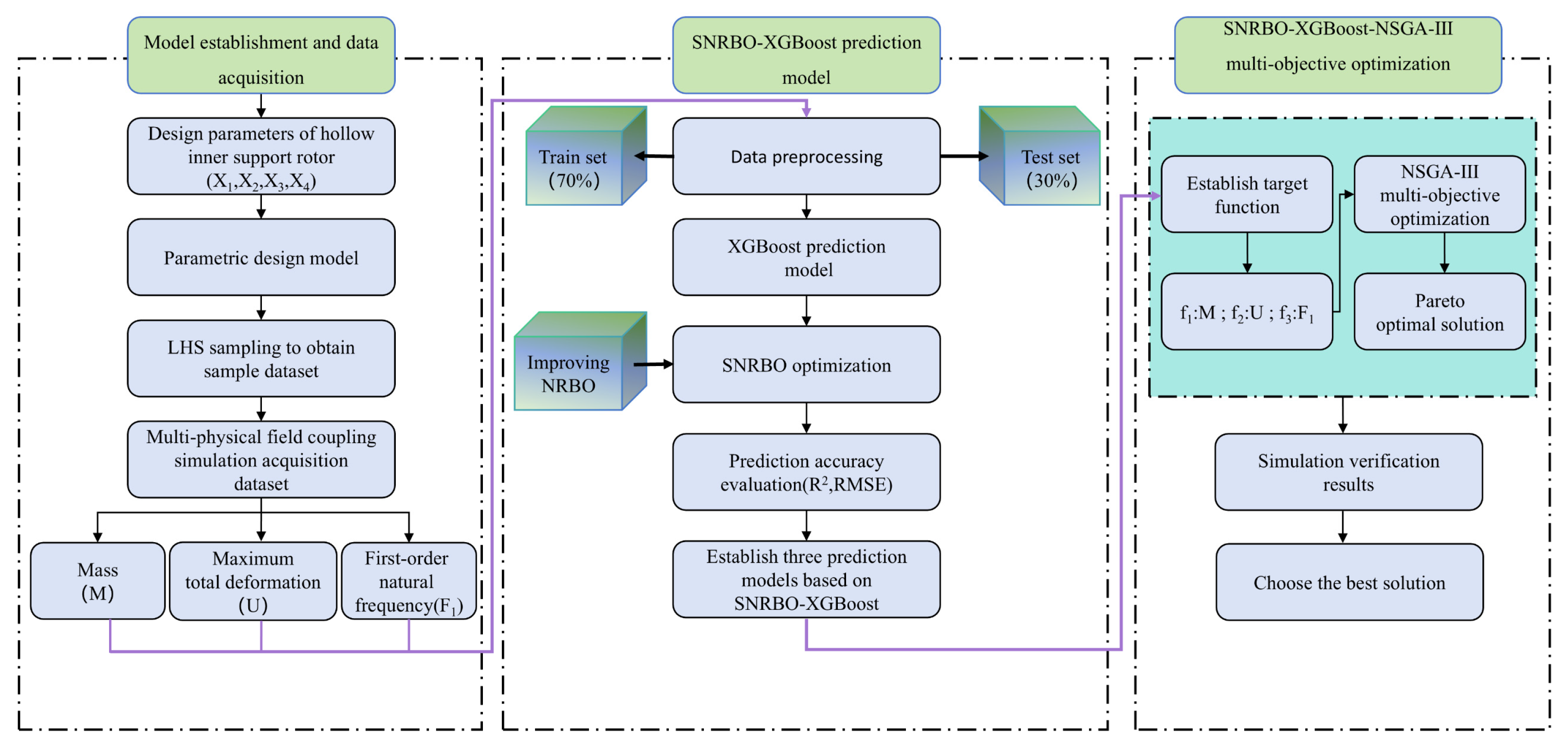
Figure 1. Multi-Objective Optimization Process for Screw Rotor Based on SNRBO-XGBoost-NSGA-III.
Processes 13 03779 g001
Figure 2. (a) shows the structure of male and female rotors, (b) the sectional view of the male rotor, and (c) the end-face sectional view of the male rotor.
Processes 13 03779 g002
Figure 3. Flowchart of the SNRBO Optimization Algorithm.
Processes 13 03779 g003
Figure 4. Convergence curves of five algorithms on CEC2022 benchmark functions.
Processes 13 03779 g004
Figure 5. NSGA-III Multi-Objective Optimization Algorithm Workflow Diagram.
Processes 13 03779 g005
Figure 6. Schematic of Boundary Constraints and Load Application in Male–Female Rotor Coupled Simulation.
Processes 13 03779 g006
Figure 7. Simulation Results of the Original Solid Rotor Model. (a) Fluid Pressure Distribution Cloud Chart. (b) Temperature Field Distribution in Steady-State Heat Analysis. (c) Total Deformation from Thermal–Fluid–Structure Coupling Calculation. (d) First-Order Natural Frequency from Modal Analysis.
Processes 13 03779 g007
Figure 8. Sample Simulation Results. (a) Total Deformation from Thermal–Fluid–Structure Coupling Calculation. (b) First-Order Natural Frequency from Modal Analysis.
Processes 13 03779 g008
Figure 9. Training Results with XGBoost Default Hyperparameters.
Processes 13 03779 g009
Figure 10. SNRBO Algorithm Iterative Optimization of Optimal RMSE.
Processes 13 03779 g010
Figure 11. Performance of SNRBO-XGBoost on Three Objective Functions.
Processes 13 03779 g011
Figure 12. Pareto Frontier Distribution of Screw Rotor Structure in Multi-Objective Optimization.
Processes 13 03779 g012
Figure 13. Simulation Validation Results of Maximum Total Deformation for the Optimal Rotor Structure.
Processes 13 03779 g013
Figure 14. Simulation Validation Results of First-Order Natural Frequency for the Optimal Rotor Structure.
Processes 13 03779 g014
Table 1. Comparison of existing lightweight screw rotor studies.
StudyStructuralOptimization MethodOptimization
Results
Comparative
Analysis
Chao [13]Equal wall thickness hollow rotorFinite element static and modal analysis comparing wall thickness designs; prioritize mass reduction while ensuring strength and modal safety.Mass reduction of 39.75%, 35.82%, and 21.04% for the three wall thickness configurations; corresponding modal frequency decreases of 7.1%, 5.8%, and 0.6%Focused on manufacturability and weight reduction; lacks systematic optimization and multi-objective strategies, limiting complex design application
Wang [14]Equal wall thickness with internal support structureRSM with FE static, modal, and FSI analysis; sequential design optimization to reduce mass first, then minimize deformation within parameter limits.Mass reduced by 27.09%, deformation increased by 2.86%Sequential optimization, single-point solution; response surface dependent, unsuitable for global multi-objective
Zhi [15]Shell–internal framework structure design integrated with additive manufacturingOrthogonal design with FE static, FSI, and thermal analysis; reduce mass first, then control deformation; emphasizes manufacturability.Mass reduced by 25.43%, static deformation increased by 7.4%Focuses on manufacturability; lacks global exploration, with analysis confined to a limited parameter range and reliant on orthogonal design, reducing optimization depth and trade-off exploration.
Present MethodParameterized modeling with internal support framework for lightweight designSNRBO surrogate modeling + NSGA-III multi-objective optimization with thermal–fluid–solid coupling; simultaneously minimize mass and deformation, maximize natural frequency.Mass reduced by 64.43%, deformation reduced by 4.41%, first natural frequency increased by 82.14%Global multi-objective framework and high-fidelity model; efficient trade-off exploration, strong engineering applicability
Table 2. Description of Design Variables and Their Ranges.
Design ParameterVariable NameUnitValue Range
Thickness of Both End FacesX1mm[5,35]
Thickness of Working Gear FaceX2mm[4–40]
Width of Internal Support RodX3mm[4–16]
Diameter of Internal Support ColumnX4mm[20–78]
Table 3. Partial Design Samples.
X1X2X3X4
31.7028.405.1041.30
14.808.808.2045.80
13.8023.709.3032.50
6.9036.1010.3060.60
6.5012.707.5075.20
Table 4. CEC2005 Test Function Information.
NO.NameDimRangefmin
F01Sphere Function30[−100,100]0
F02Schwefel’s Problem 2.2230[−10,10]0
F03Schwefel’s Problem 1.230[−100,100]0
F04Schwefel’s Problem 2.2130[−100,100]0
F05Generalized Rosenbrock’s Function30[−30,30]0
F06Step Function30[−100,100]0
F07Quartic Function, i.e., Noise30[−1.28,1.28]0
F08Shifted and rotated Levy function30[−500,500]−12,569.5
F9Shifted and rotated Schwefel’s function30[−5.12,5.12]0
F10Hybrid function 1 (N = 3)30[−32,32]0
F11Hybrid function 2 (N = 3)30[−600,600]0
F12Hybrid function 3 (N = 3)30[−50,50]0
F13Hybrid function 4 (N = 4)30[−50,50]0
F14Hybrid function 5 (N = 4)30[−65.536,65.536]0.99800383
F15Hybrid function 6 (N = 4)30[−5,5]0.0003075
F16Hybrid function 7 (N = 5)30[−5,5]−1.0316285
F17Hybrid function 8 (N = 5)30[−5,10–5,10]0.39788735
F18Hybrid function 9 (N = 5)30[−2,2]2.999999
F19Hybrid function 10 (N = 6)30[0,1]−3.8627821
F20Composition function 1 (N = 3)30[0,1]−3.3219952
F21Composition function 2 (N = 3)30[0,10]−10
F22Composition function 3 (N = 4)30[0,10]−10
F23Composition function 4 (N = 4)30[0,10]−10
Table 5. Ablation Study Results: Optimization Performance of NRBO–SNRBO5 on CEC2005.
Fun.IndicatorNRBOSNRBO1SNRBO2SNRBO3SNRBO4SNRBO5
F1min000000
avg000000
std000000
F2min000000
avg000000
std000000
F3min000000
avg000000
std000000
F4min000000
avg000000
std000000
F5min25.713727.852728.444721.472421.76899.7922
avg28.877128.585128.336122.633922.196312.7850
std1.05290.29990.16100.96060.64511.4854
F6min1.64941.46001.13861.815 × 10−51.836 × 10−56.512 × 10−23
avg2.33342.21991.52241.432 × 10−41.949 × 10−45.138 × 10−18
std0.74180.65440.51551.629 × 10−42.679 × 10−41.178 × 10−17
F7min5.654 × 10−62.522 × 10−71.074 × 10−76.652 × 10−75.367 × 10−71.882 × 10⁻⁷
avg1.688 × 10−54.191 × 10−63.691 × 10−63.478 × 10−62.504 × 10−62.431 × 10⁻⁶
std9.616 × 10−63.304 × 10−63.551 × 10−62.922 × 10−62.421 × 10−62.253 × 10⁻⁶
F8min−12,568.9012,550.975−12,358.18−12,214.164−12,451.031−12,569.486
avg−11,973.12−11,157.92−11,003.45−11,714.179−11,784.138−11,977.295
std617.53751372.64291072.1951434.0522521.7963611.6129
F9min000000
avg000000
std000000
F10min4.441 × 10−164.441 × 10−164.441 × 10−164.441 × 10−164.441 × 10−164.441 × 10⁻¹⁶
avg4.441 × 10−164.441 × 10−164.441 × 10−164.441 × 10−164.441 × 10−164.441 × 10⁻¹⁶
std000000
Table 6. CEC2017 Test Function Information.
NO.NameDimRangefmin
F01Shifted and rotated bent cigar function10[−100,100]100
F03Shifted and rotated Zakharov function10[−100,100]300
F04Shifted and rotated Rosenbrock’s function10[−100,100]400
F05Shifted and rotated Rastrigin’s function10[−100,100]500
F06Shifted and rotated expanded Scaffer’s F6 function10[−100,100]600
F07Shifted and rotated Lunacek bi_Rastrigin function10[−100,100]700
F08Shifted and rotated non-continuous Rastrigin’s function10[−100,100]800
F09Shifted and rotated Levy function10[−100,100]900
F10Shifted and rotated Schwefel’s function10[−100,100]1000
F11Hybrid function 1 (N = 3)10[−100,100]1100
F12Hybrid function 2 (N = 3)10[−100,100]1200
F13Hybrid function 3 (N = 3)10[−100,100]1300
F14Hybrid function 4 (N = 4)10[−100,100]1400
F15Hybrid function 5 (N = 4)10[−100,100]1500
F16Hybrid function 6 (N = 4)10[−100,100]1600
F17Hybrid function 7 (N = 5)10[−100,100]1700
F18Hybrid function 8 (N = 5)10[−100,100]1800
F19Hybrid function 9 (N = 5)10[−100,100]1900
F20Hybrid function 10 (N = 6)10[−100,100]2000
F21Composition function 1 (N = 3)10[−100,100]2100
F22Composition function 2 (N = 3)10[−100,100]2200
F23Composition function 3 (N = 4)10[−100,100]2300
F24Composition function 4 (N = 4)10[−100,100]2400
F25Composition function 5 (N = 5)10[−100,100]2500
F26Composition function 6 (N = 510[−100,100]2600
F27Composition function 7 (N = 6)10[−100,100]2700
F28Composition function 8 (N = 6)10[−100,100]2800
F29Composition function 9 (N = 3)10[−100,100]2900
F30Composition function 10 (N = 3)10[−100,100]3000
Table 7. Parameter Settings of Each Algorithm.
AlgorithmParameter
NRBO D F = 0.6
SSA α ( 0 , 1 ] , R 2 [ 0 , 1 ] , S T [ 0.5 , 1 ]
GWO r 1   &   r 2 [ 0 , 1 ] , C [ 0 , 2 ]
DBO k = 0.1 , λ = 0.1 , b = 0.3 , S = 0.5
Table 8. Statistical Results of Optimization Algorithms on the CEC2017 Benchmark Functions.
Fun.IndicatorSNRBONRBOSSAGWODBO
F1min100124,176.0025100817.51846173.12119
F1std336.4485452,396,364.033556.141662,984,131.26394475.46590
F1avg186.2792533,293,989.093337.874114,147,219.25995858.13815
F3min300313.9677300300.13304300
F3std091.0480601071.638550
F3avg300475.57855300852.53363300
F4min400402.19641400.00000403.14014400.07016
F4std031.14973015.4314213.38114
F4avg400430.56487400.3674412.35204406.94101
F5min504.9748516.57792503.97984504.05717504.97479
F5std8.843299.9696511.484165.954476.66001
F5avg518.97102533.57897525.30341511.03369522.70239
F6min600607.12295600.00000600.00891600.00000
F6std0.002067.804631.595850.355552.27558
F6avg600.00152619.90204601.10083600.15725602.33398
F7min713.91117730.24737731.59653712.33565708.97840
F7std7.2185121.0716123.754717.649137.46474
F7avg726.19065758.93307783.39142722.16173725.91688
F8min806.96471813.43160812.93446807.97522808.95463
F8std6.403878.969278.988233.174688.82478
F8avg818.34038827.06885823.92535809.62024822.93602
F9min900.00000905.84990900.00000900.01313900.00000
F9std5.6544767.08529354.265172.820683.68053
F9avg905.42374984.950431145.74665901.14792901.29885
F10min1133.812421421.277551280.611801015.425571147.38275
F10std270.04951250.57236240.40111251.58968253.89499
F10avg1711.609062006.604091683.821571400.527671606.67873
Table 9. Parameter Description.
NameSymbolRangeDescription
num_treesX1[30,500]Number of decision trees: Too few cause less fitting; too many increase complexity and computational cost.
max_depthX2[3,10]Maximum tree depth: Controls model complexity. Greater depth boosts fitting ability but may cause overfitting.
etaX3[0.0001,0.1]Learning rate: Controls the weight update step size per tree. Smaller values require more iterations but yield a more robust model.
Table 10. Material Properties of 316L Stainless Steel.
DensityPoisson RatioThermal Expansion CoefficientThermal ConductivityYield Strength
7.95
ρ / k g m 3
0.317.3
K 1
14
W m 1 K 1
177
M P a
Table 11. Optimized Design Variables.
Design ParameterOptimized ValueUnit
Thickness of Both End Faces27.34mm
Thickness of Working Gear Face4.11mm
Width of Internal Support Rod4.72mm
Diameter of Internal Support Column24.16mm
Table 12. Performance Comparison Between Hollow-Supported and Original Solid Structures After Optimization.
Optimization
Object
Initialization ValueOptimal
Values
Variable Quantity
Maximum total deformation (Mm)0.089230.08896−0.3%
Mass (kg)113.1444.46−60.7%
First-order Natural Frequency (Hz)302.12517.11+71.16%
Table 13. Comparison of Regression Model Prediction Accuracy on the Test Set.
Regression ModelR2RMSE
Kriging0.943, 0.990, 0.9550.0013, 2.3522, 8.0353
RBF0.819, 0.951, 0.8390.0020, 4.0443, 14.326
SNRBO-XGBoost0.978, 0.990, 0.9820.0008, 1.8084, 5.0453
Disclaimer/Publisher’s Note: The statements, opinions and data contained in all publications are solely those of the individual author(s) and contributor(s) and not of MDPI and/or the editor(s). MDPI and/or the editor(s) disclaim responsibility for any injury to people or property resulting from any ideas, methods, instructions or products referred to in the content.