Abstract
Heavy oil reservoirs often enter a high-water-cut and low-production stage after multiple cycles of steam stimulation. Converting to steam flooding can enhance recovery, yet the reliable prediction of incremental production potential and optimal design of injection–production parameters remain limited. In this study, a real heavy oil reservoir block was selected to develop a hybrid modeling framework integrating numerical simulation and machine learning for predicting steam flooding performance. A conceptual model was established on a numerical simulation platform to reproduce the transition from cyclic stimulation to continuous steam flooding, analyzing temperature, oil saturation, and recovery evolution under different geological, operational, and process conditions. Sensitive parameters were identified through single- and multi-factor analyses, and mathematical models for multiple injection–production schemes—continuous, cyclic, and asynchronous—were constructed for optimization. A comprehensive multi-scenario dataset combining simulation and field data was used to train and validate several machine learning models, including artificial neural networks, gradient boosting decision trees, XGBoost, and LightGBM. Among them, the LightGBM model achieved the highest predictive accuracy (R2 = 0.99) and computational efficiency. The proposed framework enables the rapid and reliable prediction of incremental oil potential and provides a robust tool for optimizing steam flooding parameters, offering significant value for field-scale heavy oil development.
1. Introduction
The heavy oil portion of petroleum resources is an important component of global hydrocarbon reserves, accounting for about two-thirds of the world’s oil reserves [1,2]. China’s heavy oil resources are also very abundant (over 2 × 10¹⁰ tons), representing more than 20% of the country’s total oil resources. However, heavy oil reservoirs typically have shallow burial depths and low formation temperatures, and crude oil has high viscosity and contains large amounts of resins and asphaltenes, resulting in poor formation mobility and limited natural energy [3,4]. For such thin, shallow heavy oil reservoirs, cyclic steam stimulation is commonly used in the early stages of development to enhance production. After multiple cycles of steam stimulation, however, a series of problems often arise: because of strong heterogeneity, high steam-to-oil mobility ratios and large steam–liquid density contrasts, the injected steam chamber is confined to the near-well region, and large volumes of oil in the far field remain immobile; injected steam also tends to channel through high-permeability pathways (steam fingering), causing a sharp decline in cyclic recovery performance [5,6]. As a result of these factors, after multiple steam cycles, well fluid water cuts increase markedly, per-cycle oil production decays rapidly, the oil-to-steam ratio drops significantly, and the economics of development deteriorate. Actual statistics show that recovery factors achieved by cyclic steam stimulation in heavy oil reservoirs are typically less than 25% [7,8]. Therefore, once cyclic steam stimulation enters a high-water-cut, low-production stage, converting to steam flooding development becomes a necessary means to improve the ultimate recovery of heavy oil reservoirs [9,10].
As a follow-up measure after cyclic steam stimulation to further increase recovery, both theory and field tests indicate steam flooding can raise recovery by roughly an additional 30 percentage points on top of cyclic steam results [11,12]. However, field outcomes in some oilfields have been disappointing: due to insufficient understanding of the conditions and parameters required for conversion to steam flooding, implementations are often undertaken blindly, and improper choices of injection–production parameters (e.g., steam injection rate, timing of the switch from cyclic steaming to steam flooding) lead to steam flood performance below expectations [13,14]. The reasons are twofold. On the one hand, there is currently no efficient and accurate quantitative method to characterize the potential incremental recovery from converting to steam flooding after multiple cyclic stimulations, leaving decisions on whether and when to implement steam flooding without a scientific basis. On the other hand, research on optimizing injection–production parameters for steam flood designs is relatively weak: existing methods typically target a single mode and do not adequately consider differences among injection–production schemes, nor do they provide differentiated optimization of well-level parameters to achieve balanced and synergistic inter-well displacement [14,15]. Traditional steam flood potential prediction relies mainly on numerical simulation using specialized thermal reservoir simulators; the simulation process is time-consuming and costly [16]. Conventional parameter-optimization methods (such as analogy methods, empirical formulas, and orthogonal experimental design) struggle with complex and variable reservoir conditions, and although intelligent optimization methods have been applied, they remain limited to optimizing single injection–production schemes and cannot comprehensively guide parameter design across multiple modes [16,17]. These technical challenges and research gaps severely constrain the effectiveness of steam flooding in improving recovery from heavy oil reservoirs.
In recent years many researchers have conducted extensive studies on evaluating steam flood potential and on parameter optimization for heavy oil. For feasibility and performance prediction of steam flooding, various approaches have been proposed, including analytical models to infer steam flood dynamics [18,19,20,21], empirical correlation formulas, laboratory physical simulation experiments [22,23], and numerical simulation techniques to predict recovery and oil-to-steam ratios [24]. For example, Shutler [24] introduced a two-dimensional model that accounts for heat conduction and convection when determining the temperature distribution to simulate oil, water, and gas phases in sandstone. Abdalla and Coats [25] were among the first to use numerical methods to inject steam into sandstone by solving a set of governing differential equations. Assuming compressible fluids, they adopted an implicit-pressure, explicit-saturation (IMPES) technique to obtain pressures and saturations for all three phases. Based on their results, a model was developed to determine steam condensation rates for heat-transfer calculations. Coats et al. [26] developed a 3D model for the numerical simulation of steam injection in sandstone, including mass and energy balances in both the reservoir and the overburden. Their solution did not require iterative procedures when accounting for compressibility, reducing computational work at a time when runtime was a critical constraint. Ferrer and Farouq Ali [27] used a numerical model to study mass and heat transfer between phases in multicomponent flow, simulating three-phase, three-dimensional flow during steam injection into sandstone. Coats [28] used an implicit model to simulate distillation and solution-gas phenomena in steam flooding; the model included all terms related to solution gas, distillation, and capillary pressure to study saturation and composition changes under the assumption of thermodynamic equilibrium. In addition to modeling work, many researchers—such as Sumnu et al. [29], Mollaei et al. [30], and Souraki et al. [31]—have carried out systematic laboratory experiments. These lab studies have mainly focused on parameter sensitivity analysis to capture the key aspects of steam flood processes. Overall, existing research has offered multiple approaches for evaluating steam flood potential, but efficient quantitative prediction methods are still lacking.
Heavy oil reservoirs represent an important unconventional energy resource that requires efficient thermal enhanced oil recovery (EOR) techniques to overcome challenges associated with high viscosity and low mobility. Among various thermal EOR methods, Cyclic Steam Stimulation (CSS) and steam flooding are widely used to improve oil mobility by injecting heat into the reservoir. CSS involves repeated cycles of steam injection, soaking, and production from the same well (the “huff-and-puff” process), while continuous steam flooding aims to maintain reservoir temperature and pressure by displacing oil with steam. Understanding the potential conversion from CSS to different steam flooding modes is therefore essential for optimizing the recovery process in heavy oil reservoirs. In recent years, numerous studies have explored the mechanisms and performance of steam injection through both field applications and numerical simulations. Advanced thermal simulators such as CMG-STARS have been extensively used to study steam chamber development, heat transfer, and production dynamics under various operational parameters. However, numerical simulation is often computationally expensive, particularly when conducting multi-parameter optimization and uncertainty analysis. These limitations highlight the need for efficient, data-driven approaches that can complement or accelerate conventional numerical methods. The rapid development of data-driven modeling and machine learning (ML) techniques has provided new opportunities to improve prediction and optimization in reservoir engineering. ML methods such as artificial neural networks (ANNs), support vector machines (SVMs), gradient boosting decision trees (GBDTs), and convolutional neural networks (CNNs) have been successfully applied to forecast oil production, evaluate recovery factors, and optimize steam injection performance. For example, supervised learning and ensemble algorithms have been used to capture complex nonlinear relationships between reservoir parameters and production responses, while clustering and pattern recognition methods help identify key influencing factors. These approaches greatly reduce computational cost and enable faster decision-making compared to purely physics-based simulation models. Although existing ML-based research has made considerable progress, several critical gaps remain. Most studies have focused on a single recovery process—such as CSS or SAGD (Steam-Assisted Gravity Drainage)—and have not established a unified workflow capable of analyzing and optimizing multiple steam flooding modes. Moreover, many studies treat simulation and ML as separate tools, without coupling them in an integrated workflow that ensures both predictive accuracy and optimization efficiency. Consequently, there is still a lack of a comprehensive methodology that combines physical simulation, data-driven prediction, and intelligent optimization for heavy oil steam flooding.
To address these limitations, this study proposes a hybrid numerical–machine learning framework for evaluating the potential and optimizing the parameters of different steam flooding methods in heavy oil reservoirs. First, a series of thermal numerical simulations are performed to analyze the incremental oil recovery potential when converting from CSS to various steam flooding strategies. The simulation results are then used to train ML surrogate models that rapidly predict recovery performance from reservoir and operational parameters. Finally, the Bayesian Adaptive Direct Search (BADS) algorithm is integrated to optimize injection and production parameters for multiple steam flooding scenarios—continuous, intermittent, asynchronous, and hybrid modes—aimed at maximizing the net present value (NPV) under practical constraints. This integrated workflow effectively combines the strengths of physics-based simulation, machine learning prediction, and intelligent optimization. The numerical simulations ensure physical fidelity, ML surrogates provide computational efficiency, and the BADS algorithm delivers reliable global optimization. Overall, this study contributes a data-driven and physics-guided framework that enables rapid evaluation, potential prediction, and optimization of heavy oil steam flooding processes, offering both methodological innovation and practical guidance for multi-scenario field applications.
2. Materials and Methods
2.1. Factors Affecting Steam Flood Potential
In the late stages of cyclic steam stimulation, uneven heat distribution and a reservoir energy deficit occur; converting to steam flooding can improve heat utilization, replenish energy, mobilize remaining oil, and thereby significantly increase recovery. To predict the incremental potential, geological, development and process factors must be considered together, and key parameters screened to ensure prediction accuracy. Using numerical simulation, the effects of each factor on the temperature field and oil saturation are analyzed, and the incremental oil, oil displacement rate and recovery improvement are evaluated; finally, multivariate analysis is used to identify the main controlling factors.
2.1.1. Establishment of the Numerical Simulation Model
The N reservoir is located at the southwestern end of the Shijiutuo uplift. It is a complex nose-shaped structure comprising three types of traps: a half-anticline, complex fault blocks, and slope traps. Proven geological oil reserves in the reservoir are 3.169 × 10⁴ m3 (3.169 × 10⁷ m3). The N reservoir is a complex field with multiple oil-bearing units and multiple oil–water systems. Well-log data indicate that in the southern area, the lower section of the Minghuazhen Formation has porosities ranging from 28% to 41%, with an average of 38%; permeability ranges from 350 to 14,300 × 10−3 μm2. The reservoir is buried at 500–700 m, with an effective thickness of 3–7 m. Closure areas range from 30.7 to 68.3 km2, and closure heights (amplitudes) range from 110 to 450 m. The reservoir is characterized mainly by high porosity and high permeability, and the fluids are heavy oil. The target horizon’s average oil temperature is 56 °C and the formation pressure is 6.07 MPa; the oil viscosity at 56 °C is 56,000 mPa·s (live oil viscosity). In the southern area, the lower Minghuazhen reservoir displays normal graded (fining-upward) sedimentary characteristics in its lithologic profile. Sandstone composition in the lower Minghuazhen ranges as follows: quartz 37–41%, feldspar 32–39%, and lithic fragments 21–30%—primarily lithic-feldspathic fine-grained sandstone. Thin-section analysis shows median grain sizes between 0.1 and 0.2 mm, with an average of 0.15 mm. The southern area of the N reservoir is divided into three oil units—K0, KI, and KII—with the main reservoirs occurring in K0 and KI, accounting for 97% of the block’s reserves. In this study, a steam flood numerical simulation model for an N heavy oil reservoir was built using tNavigator 23.4 (Figure 1) to accurately represent the flow, heat conduction, and phase-change behavior of high-viscosity crude. Model construction included 3D geological modeling, grid discretization, well placement and local refinement, yielding 168,320 grid cells that reasonably balance accuracy and computational efficiency. A black-oil fluid model was used to describe the PVT properties of the heavy oil, and multiphase flow parameters for oil, water and gas were calibrated against field relative-permeability and viscosity-versus-temperature curves (Table 1 and Figure 3) to ensure the properties realistically reflect reservoir conditions. Figure 3a shows the oil–water relative permeability curves, which reflect how the mobilities of the oil and water phases change with water saturation. As water saturation increases, the oil relative permeability gradually decreases while the water relative permeability rises rapidly. Figure 3b is the water-phase compressibility curve, showing the relationship between formation water compressibility and pressure. The curve declines approximately linearly, indicating that formation water is weakly compressible and stable within the conventional pressure range. Figure 3c is the oil phase compressibility curve, describing how crude oil compressibility varies with pressure. The curve decreases gradually with increasing pressure, implying that crude oil is more compressible at low pressures but tends to stabilize under high-pressure conditions; this behavior reflects the significant influence of dissolved gas, since higher pressure produces smaller oil volume changes. Figure 3d is the oil viscosity–temperature curve, showing that crude oil viscosity falls rapidly as temperature increases and levels off above about 80 °C, indicating high temperature sensitivity and that heating aids mobility. Figure 3e is the gas phase compressibility curve, which shows that compressibility is large at low pressures, decreases rapidly with increasing pressure, and then stabilizes—suggesting that the gas approaches ideal gas behavior at high pressure. Figure 3f is the gas density curve: gas density increases markedly with pressure and follows an approximately exponential trend, demonstrating the strong compressibility of gas, where higher pressure reduces intermolecular spacing and rapidly increases density. The model includes 98 wells, with well types comprising horizontal and vertical wells. It comprehensively considers formation temperature and pressure boundaries and the well pattern layout, providing a reliable basis for subsequent studies of steam flood development behavior and scheme optimization.
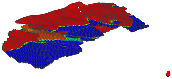
Figure 1.
3D geological model of the N reservoir.

Table 1.
Basic parameters.
Based on the existing field model, a numerical simulation model was built by selecting a representative area and typical well locations, as shown in Figure 2. It includes nine steam stimulation production wells; the horizontal section length of each horizontal well is 200 m. Development was carried out using an aligned row well pattern with three rows, three wells per row, and a row spacing of 120 m.

Figure 2.
Two-dimensional diagram of the injection–production model.
Figure 2.
Two-dimensional diagram of the injection–production model.


Figure 3.
Basic reservoir property plots should be listed as: (a) oil–water relative permeability; (b) water phase compressibility; (c) oil phase compressibility; (d) oil viscosity–temperature curve; (e) gas phase compressibility; (f) gas density.
Figure 3.
Basic reservoir property plots should be listed as: (a) oil–water relative permeability; (b) water phase compressibility; (c) oil phase compressibility; (d) oil viscosity–temperature curve; (e) gas phase compressibility; (f) gas density.

2.1.2. Analysis of Geological Factors
Single-factor numerical simulations were conducted on the conceptual model, using incremental oil from the measure, oil produced per unit steam (oil/steam replacement rate), and recovery improvement as evaluation metrics to assess geological sensitivity for converting the target area from cyclic steam stimulation to steam flooding. The simulation procedure was as follows: perform multiple steam cycles until daily oil production falls below 3 m3·d−1, then switch to steam flooding; a cumulative oil-to-steam ratio of 0.12 is taken as the limiting production at which wells are shut in. All scenarios were run with the same operating conditions and durations for comparison. Figure 4 shows the effects of geological factors on steam flood potential. Results indicate that effective reservoir thickness is positively correlated with incremental oil and the oil/steam replacement rate, but negatively correlated with recovery factor. Under burial depths of 200–1000 m, increasing depth raises formation temperature and pressure more than it reduces oil heating efficiency and volumetric effects, producing slight improvements in all three indicators. As porosity increases from 0.10 to 0.30, incremental oil and the oil/steam replacement rate increase markedly, while the recovery factor gain decreases; the mechanism is similar to that for thickness. Increasing permeability in the range 3000 × 10−3–15,000 × 10−3 μm2 noticeably improves flowability and steam sweep, raising all three indicators, but marginal benefits diminish beyond about 12,000 × 10−3 μm2. Increased heterogeneity (coefficient of variation 0.10–0.30) promotes steam channeling and reduces swept volume, decreasing the indicators, though the effect levels off once high-permeability channels form. When crude viscosity rises from 20,000 to 320,000 mPa·s, flowability and heat transfer become severely constrained and the three indicators fall rapidly at first and then stabilize; very high viscosity effectively reduces the available pore volume and limits steam flood efficiency.
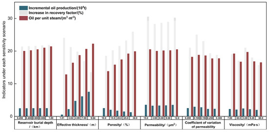
Figure 4.
Influence of geological factors on steam flood potential.
2.1.3. Analysis of Development Factors
Figure 5 shows the influence of development factors on steam flood potential. To assess the incremental potential of switching to steam flooding after multiple cycles of steam stimulation, this study selected dynamic development indicators—water cut, reservoir pressure, formation temperature, remaining recoverable reserves, degree of depletion, and daily oil rate—and used an equivalent-state approach, whereby production dynamics corresponding to different stimulation cycles were taken as representative states, and switching-to-steam flood numerical simulations were carried out on those states to indirectly examine the effect of each factor. Evaluation metrics were incremental oil, oil per unit steam (oil/steam replacement rate), and recovery factor improvement, with temperature and saturation fields analyzed to reveal the physical mechanisms. The results show that, within certain ranges, higher water cut enhances mobility and heat transfer, increasing all three metrics; reduced reservoir pressure favors steam injection and energy utilization, significantly improving displacement efficiency; and a higher formation temperature lowers oil viscosity and improves mobility, thereby boosting incremental potential. As the remaining recoverable reserves decrease, incremental oil and recovery gains decline while the oil/steam replacement rate rises, indicating an optimal reserve interval. A greater degree of depletion reduces all three metrics, showing that high depletion limits further incremental potential. The effect of daily oil rate on potential is hump-shaped (rises then falls), but relatively small in magnitude: higher early-stage daily output helps connectivity and steam injection, while reduced remaining oil later weakens the effect, so daily oil rate is a secondary reference indicator. In summary, development dynamics significantly affect the potential for converting to steam flooding, primarily by controlling steam injectability, thermal efficiency, and the distribution of remaining oil.
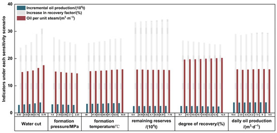
Figure 5.
Influence of development factors on steam flood potential.
2.1.4. Analysis of Process Parameter Factors
Figure 6 shows the effect of process factors on steam flood potential. Although cyclic steam operational parameters are numerous, their effects ultimately show up in production dynamics; therefore, this study focuses on well spacing as a key engineering parameter. Numerical simulations were conducted for paired horizontal well groups with spacing of 100–300 m while keeping other conditions constant, to compare incremental oil, oil-per-unit-steam (oil/steam replacement rate), recovery improvement, and saturation-field changes. The results indicate that as spacing increases, incremental oil and recovery gains first rise and then fall, whereas the oil/steam replacement rate declines continuously. Moderately increasing spacing can enlarge the reserve volume controlled by a single well and boost incremental potential; however, excessive spacing leads to insufficient steam sweep, reduced thermal sweep area and displacement efficiency, and weakened performance. The saturation fields also show steam coverage declines significantly with larger spacing. Therefore, well spacing has a significant impact on the potential of switching to steam flooding; a balance must be struck between reserve scale and thermal sweep, and development efficiency under wide spacing can be improved by optimizing well patterns and adjusting injection–production parameters.
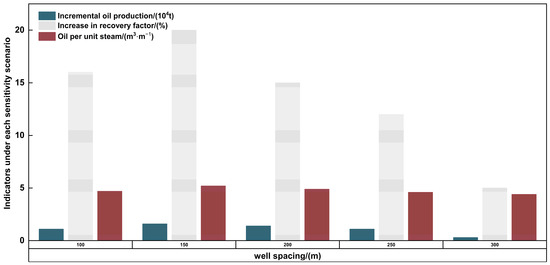
Figure 6.
Effect of process factor (well spacing) on steam flood potential.
2.1.5. Comprehensive (Integrated) Analysis of Parameter Factors
The potential for switching to steam flooding is affected by multiple factors and cannot be assessed by any single factor alone. Therefore, multivariate analysis based on single-factor studies is necessary. Grey relational analysis (GRA) is a commonly used multivariate method that quantifies the influence of each factor in a system by computing their degrees of association. The core idea of GRA is that if two factors exhibit similar variation trends, their degree of association is high; otherwise it is low. This method is well suited to studying the multivariable influences during the transition to steam flooding and can quantify the specific impact of each factor on development potential.
To further investigate the potential of converting to steam flooding, numerical simulation models of well-group transitions from cyclic steam stimulation to steam flooding were built under different geological, development, and process conditions. The simulation results cover the conversion under 14 different conditions, as detailed in Figure 7. The figure shows the influencing factors, including net-to-gross ratio (NTG), reservoir pressure (P), porosity (φ), water cut (fw), reservoir thickness (H), permeability coefficient of variation (V), reservoir temperature (T), degree of depletion (R), well spacing (S), permeability (K), daily oil rate (Or), and remaining reserves (Res).
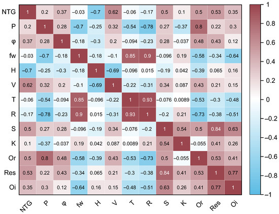
Figure 7.
Incremental steam flood recovery and influencing factors.
To analyze the influence of each factor, the recovery factor increase was chosen as the reference sequence and the other influencing parameters were used as comparison sequences. The data series were nondimensionalized using the mean method. Grey relational coefficients for each factor were calculated and then converted to grey relational grades; the ranking of these grades is shown in Figure 8. The ranking indicates that, among factors affecting the potential of switching to steam flooding, remaining reserves have the greatest impact on recovery gain, followed by net-to-gross ratio, reservoir thickness, and permeability coefficient of variation. Factors with relatively small influence include reservoir burial depth, porosity, and daily oil rate, so they can be omitted in subsequent studies. Considering that effective reservoir thickness is defined as the product of net-to-gross ratio and reservoir thickness, it is recommended to combine these two parameters into a single factor. Thus, the key factors for further study are effective thickness, permeability coefficient of variation, water cut, formation temperature, reservoir pressure, degree of depletion, remaining reserves, and well spacing.
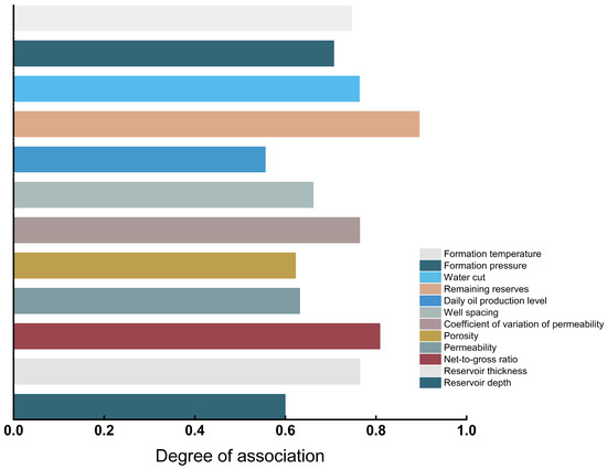
Figure 8.
Degrees of association and ranking.
2.2. Principles of Machine Learning Methods
The factors influencing the potential of converting to steam flooding are numerous and diverse. The impact on steam flooding potential is not the result of a single factor, but rather the combined effect of multiple factors. There exists a complex nonlinear relationship between various geological, development, and process-related factors and steam flooding potential. How to quantitatively describe such complex nonlinear relationships has become an urgent problem to solve. Since the 1990s, statistical machine learning methods have developed rapidly, showing unique advantages in handling problems involving large datasets, high dimensionality, and nonlinearity. In order to further quantify the steam flooding conversion potential, machine learning methods are introduced to regress the influence of different factors on steam flooding potential. Machine learning utilizes existing data to improve specific algorithm performance through experiential learning, enabling effective responses to new environments. Therefore, four widely used and representative algorithms were selected, and their respective principles and strengths were introduced.
2.2.1. Artificial Neural Network (ANN)
An artificial neural network (ANN) is composed of many interconnected computational units designed to emulate information transmission in biological neural systems. A typical M–P (McCulloch–Pitts) neuron forms an output by weighting inputs, comparing the sum to a threshold, and passing the result through an activation function [32]. Multilayer neurons are connected in a hierarchical structure: forward propagation computes outputs, and backpropagation updates weights using gradients of a loss function, enabling complex nonlinear mappings. ANNs excel at fitting complex relationships but are sensitive to sample size and hyperparameters, are prone to overfitting, and generally lack interpretability [33]. In tabular regimes with modest sample sizes and limited feature engineering headroom, ANNs are prone to optimization instability and overfitting, require delicate regularization, and offer weaker direct interpretability—all consistent with their inferior held-out accuracy observed here. Using ANN establishes that “more flexible” does not mean “more suitable” for this domain.
2.2.2. Gradient Boosting Decision Tree (GBDT)
GBDT (Gradient Boosting Decision Tree) is a stagewise additive ensemble method based on CART regression trees that represents the prediction as a sum of many trees. The model iteratively minimizes a regularized objective function, fitting, at each step, a function in the direction of the negative gradient of the residuals from the previous round, and uses a learning rate to scale each tree’s contribution [34]. It is robust to heterogeneous features and missing values and is insensitive to feature scaling, making it well suited for structured data. However, as the number of trees and sample size grow, training cost increases substantially, so a trade-off between learning rate and model complexity is required to maintain generalization. Classical GBDT provides a strong structured data baseline, insensitivity to feature scaling, and resilience to outliers/missingness. It tests whether additive trees alone (without modern regularization/sampling innovations) can meet accuracy/efficiency targets. Its middling performance quantifies the benefit of later algorithmic advances.
For a dataset containing features and examples, , the output is predicted as the sum of additive functions:
In the equation, denotes a tree with terminal nodes; denotes the partition region defined by the terminal node of the tree. denotes the expansion coefficient obtained jointly with by fitting the training dataset through minimization of the regularized objective function,
In the equation, is a differentiable loss function.
The loss is minimized by iteratively adding leaf nodes, thereby performing gradient descent; its mathematical expression is
In the expression, is the shrinkage factor in the range (0, 1] that controls the learning rate of the training process. Empirically, smaller values of help regularize the model and thus improve generalization.
2.2.3. Extreme Gradient Boosting (XGBoost)
XGBoost is a supervised learning algorithm. XGBoost introduces second-order optimization, explicit regularization, and shrinkage, improving bias–variance trade-offs on nonlinear tabular tasks. In our results it markedly tightens training/test scatter around the 45° line, demonstrating robust generalization. It serves as a high-accuracy comparator and confirms that boosting families align with the physics-informed, interaction-rich nature of the problem. It ensembles multiple classification and regression trees (CART) to form a classifier with strong generalization ability. Each CART consists of a root node, a set of internal nodes, and a set of leaf nodes [35] (see Figure 9a). For a given dataset composed of samples and feature variables, XGBoost’s output is the sum of the predictions of CARTs (see Figure 9b); its mathematical model is
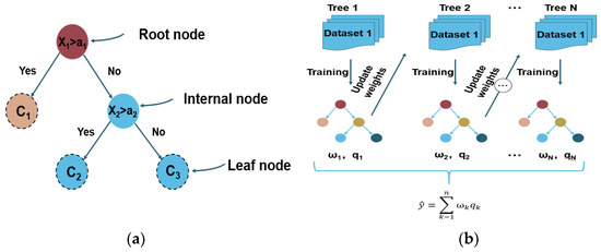
Figure 9.
Schematic of the decision tree models. (a) Schematic of the CART mode; (b) schematic of the XGBoost prediction model.
In the equation, is the th individual tree; is the output computed by the XGBoost ensemble. The CART tree function space is expressed by Equation (6):
In the equation, is the decision rule that maps an example to a (binary) leaf index; denotes the set of scores for the leaves; is the number of leaf nodes; and denotes the weight of a leaf.
To construct the prediction model , the following objective function must be minimized:
In the equation, is a differentiable convex loss function; is the regularization term that constrains model complexity; is the coefficient for the loss function; is the coefficient for the regularization term; and denotes the leaf weights.
2.2.4. Light Gradient Boosting Machine (LightGBM)
LightGBM is Microsoft’s efficient implementation of the GBDT framework, designed to address efficiency and scalability for large-scale data training [36]. LightGBM preserves the representational strengths of boosted trees while adding histogram-based splits, Gradient-based One-Side Sampling (GOSS), and Exclusive Feature Bundling (EFB). These mechanisms (i) reduce memory and training cost; (ii) prioritize high-gradient samples to focus learning where residuals are largest; and (iii) curb effective dimensionality when features are sparse or weakly overlapping. This is especially advantageous for our iterative simulation–optimization loop, where models must be retrained/tuned repeatedly. Empirically, LightGBM achieved the lowest MAE/RMSE and the highest R2 on the held-out set (≈0.977) while cutting training time substantially relative to XGBoost—thereby satisfying both predictive and operational criteria. Its core optimizations are shown in Figure 10 as follows:
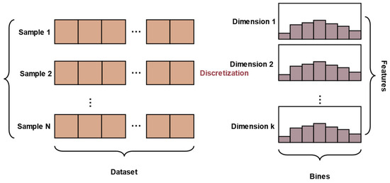
Figure 10.
Schematic of LightGBM histogram optimization.
- (1)
- Histogram algorithm.
Discretize continuous features into intervals (bins), which significantly reduces the number of passes and memory consumption, and accelerate computation by using histogram subtraction between parent and child;
- (2)
- Depth-first split strategy. prioritize splitting the leaf with the largest gain to more quickly reduce training error, but combine this with regularization parameters to prevent overfitting in Figure 11 as follows [37];
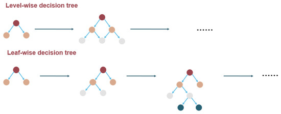 Figure 11. Comparison of different decision tree growth modes.
- (3)
- Gradient-based One-Side Sampling (GOSS). Retain samples with large gradients, randomly down sample samples with small gradients and adjust their weights, thereby reducing the number of samples while preserving accuracy [38];
- (4)
- Exclusive Feature Bundling (EFB). For high-dimensional sparse data, merge mutually exclusive or low-conflict features to reduce dimensionality and computation. With these optimizations, LightGBM greatly improves training speed and resource utilization while maintaining predictive accuracy [39].
Given (i) the tabular, interaction-heavy nature of the predictors, (ii) the need for high accuracy under limited computation budgets within a simulation-coupled workflow; and (iii) empirical superiority across multiple error metrics and runtime, LightGBM is the primary model of record. XGBoost serves as a robustness benchmark, GBDT as a classical reference, and ANN as a nonlinear baseline demonstrating that neural networks are not necessarily optimal for this domain. This portfolio is thus mechanistically and empirically justified for predicting steam flood incremental potential and optimizing field-scale development parameters.
2.3. Construction of the Prediction Model for Switching to Steam Flooding After Multiple Stimulation Cycles
2.3.1. Inputs and Outputs of the Potential-Prediction Model
The base data come from actual well-log records of 98 production wells in Reservoir N. The block is a thin, high-viscosity reservoir, and the geological model was constructed using a sequential Gaussian–Bayesian method. To ensure the representativeness of the dataset, 400 seed models were randomly selected from the geological model, covering heterogeneity in top depth, effective thickness, porosity, and permeability. On this basis, numerical simulation models were built to further evaluate the potential of switching to steam flooding. The main factors affecting the incremental production potential of converting to steam flooding after multiple huff-and-puff cycles include effective thickness, coefficient of variation of permeability, water cut at the time of conversion, reservoir temperature, reservoir pressure, degree of depletion, remaining reserves, and well spacing. Among these factors, effective thickness and the permeability coefficient of variation are geological parameters, while the others are development and operational parameters. In the numerical simulations, the geological model is represented by average effective thickness, and the permeability coefficient of variation is calculated from the relevant formulas. Development parameters such as remaining reserves, water cut, reservoir temperature, and pressure are dynamic and are recorded in real time; well spacing is treated as an operational parameter and its effect is simulated by adjusting the grid size along the x-direction in the numerical model.
Steam huff-and-puff numerical simulations were performed on the 400 generated numerical models. To assess the full-cycle potential of converting to steam flooding after multiple huff-and-puff rounds, conversion-to-steam flood simulations were carried out after different numbers of cycles; production was stopped when the cumulative oil-to-steam ratio reached the limit value of 0.12. A steam huff-and-puff numerical model with the same production time was then compared with the recovery of the post-cycle conversion-to-steam flood model, and the increase in recovery due to conversion to steam flooding—i.e., the conversion potential—was calculated.
2.3.2. Data Preprocessing
The input parameters for the potential prediction model include three categories—geological, development, and operational/process parameters—eight specific parameters in total (see Table 2). Based on the aforementioned 400 geological models, their geological parameters were calculated and then randomly entered into a database. For each geological scenario, steam huff-and-puff to steam flood numerical simulations were performed under different development conditions corresponding to 3 to 25 cycles. The outputs of each simulation case under the various scenarios included the incremental oil attributable to conversion to steam flooding. By building 8800 numerical simulation models and running 17,600 simulation runs, 4981 valid samples were generated. After completing the simulations, the dataset was cleaned and outliers were removed, leaving 4981 valid samples. The selection and elimination of samples are mainly based on ensuring a uniform distribution across geological parameters, development parameters, and process parameters, while removing data points that do not conform to historical production data, so as to ensure the applicability of the data. Each sample includes the geological, development, and operational parameters that affect the conversion-to-steam flood potential and the corresponding increase in recovery from conversion to steam flooding; these samples provide the necessary training data for machine learning models.
Table 2.
Schematic of LightGBM histogram optimization.
3. Results and Discussion
3.1. Injection–Production Schemes for Switching to Steam Flooding After Multiple Huff-and-Puff Cycles
For the five injection–production schemes for switching to steam flooding (continuous injection, intermittent injection, asynchronous injection–production, continuous injection followed by intermittent injection, and continuous injection followed by asynchronous injection–production), mathematical optimization models for injection–production parameters were developed and solved using intelligent optimization algorithms, and a collaborative intelligent optimization method for these parameters after multiple huff-and-puff cycles was proposed.
3.2. Data Preprocessing and Tuning of Controllable Parameters for Machine Learning Algorithms
3.2.1. Selection of Machine Learning Algorithms
In the study of predicting steam flood potential after multiple huff-and-puff cycles, to improve prediction accuracy and robustness we compared four commonly used machine-learning algorithms: artificial neural network (ANN), gradient boosting decision trees (GBDT), extreme gradient boosting (XGBoost), and LightGBM. The data came from the constructed dynamic production database, containing 4981 valid samples, which were randomly split into a training set (60%) and a test set (40%). Having too large a training set and too small a test set can lead to the following: the assessment of the model’s generalization ability becomes unreliable; with a large amount of training data, the model may perform extremely well on the training set, but with too few test samples, it is difficult to detect whether the model performs poorly on a broader range of data; too little test data makes the evaluation results statistically less reliable, making it difficult to perform significance testing or variance analysis; a test set that is too small may miss potentially hard-to-predict samples or edge cases, causing the model to perform poorly when encountering such situations in practical applications. Conversely, having too small a training set and too large a test set can cause the following: insufficient training data makes it difficult for the model to capture patterns or characteristic features in the data; although a large test set yields relatively stable evaluation results, the model’s overall performance remains low due to inadequate learning; a small training set easily leads to large biases in feature weights and parameter estimates; excessive data being used for testing rather than training means the available information is not fully utilized to improve the model’s capabilities. In this experiment, selecting 60% of the data as the training set and 40% as the test set was determined, after testing, to be the optimal solution. Inputs covered three categories of features—geological, development, and operational—and the outputs were incremental oil from the measure, steam-to-oil ratio, and recovery improvement.
First, the data were fed into an ANN and hyperparameters were tuned using five-fold cross-validation. Despite trying different numbers of hidden-layer nodes and combinations of activation functions, the model predictions deviated considerably from the observed values (see Table 3 and Figure 12); the data points did not cluster near the ideal 45° line, indicating that this algorithm had limited predictive ability for the problem in this study. The red line in the figure represents the trend line of the dataset. By observing the offset angle between the red line and the 45-degree line, one can intuitively assess the degree of deviation in the dataset.
Table 3.
Hyperparameters for different machine learning models.
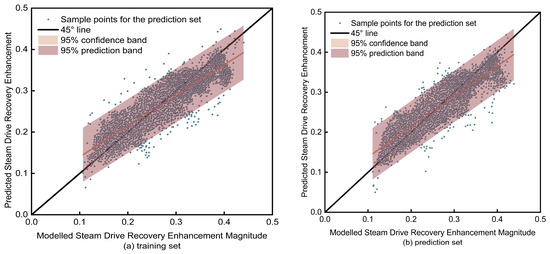
Figure 12.
Scatter plot of ANN-predicted vs. actual steam-drive potential. (a) Training set; (b) prediction set.
Next, GBDT was used to model the data. By tuning parameters such as learning rate, tree depth, and number of weak-learner iterations, the model’s performance improved slightly over the ANN, but the fit on the training and test sets remained unsatisfactory, indicating insufficient generalization in Figure 13 as follows.
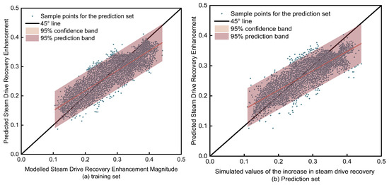
Figure 13.
Scatter plot of GBDT-predicted vs. actual steam-drive potential. (a) Training set; (b) prediction set.
Further applying the XGBoost algorithm in Figure 14 as follows, the results show that the training set data points are highly concentrated along the 45° line; although the test set exhibits slight dispersion, it remains relatively tight overall, indicating good robustness and generalization and prediction accuracy that is significantly better than the previous two methods.
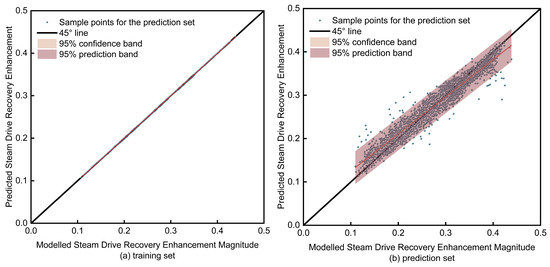
Figure 14.
Scatter plot of XGBoost-predicted vs. actual steam-drive potential. (a) Training set; (b) prediction set.
Building on this, the LightGBM algorithm was introduced. LightGBM substantially improves modeling efficiency through histogram optimization, exclusive feature bundling, and a depth-first tree-growth strategy. Using random search combined with five-fold cross-validation to tune key hyperparameters (learning rate, tree depth, number of trees), the optimal combination was found to be max depth = 3, learning rate ≈ 0.046, and 4000 trees. Under these settings, training-set predictions lie tightly along the 45° line and the test-set performance is also relatively robust, with only a few outliers; overall predictive accuracy is high (see Figure 15 and Table 4). Compared with XGBoost, LightGBM achieves comparable predictive accuracy while reducing training time from several hours to under half an hour, demonstrating a clear efficiency advantage.

Figure 15.
Scatter plot of LightGBM-predicted vs. actual steam-drive potential: (a) training set; (b) prediction set.
Table 4.
The five LightGBM hyperparameter combinations with the highest R2 predictive accuracy selected via five-fold cross-validation and random search.
To further validate the algorithms’ performance, an evaluation matrix including mean absolute error (MAE), mean relative error (MRE), root mean square error (RMSE), and coefficient of determination (R2) was constructed. The results show that ANN has the highest MAE, MRE, and RMSE and the lowest R2, i.e., the worst predictive performance; GBDT is intermediate; XGBoost achieves high accuracy and strong robustness; and LightGBM performs best among the four, with the smallest MAE, MRE, and RMSE and the largest R2 (see Figure 16). Combining qualitative and quantitative results, the ranking of predictive ability for steam flood potential after multiple huff-and-puff cycles is LightGBM > XGBoost > GBDT > ANN.
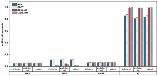
Figure 16.
Summary of evaluations of different artificial intelligence methods.
Further analysis indicates that tree-based ensemble learning methods outperform the neural network model for this problem. Their sequential boosting strategy increases the weights of error samples to continually strengthen learning, effectively controlling overfitting and improving generalization. At the same time, LightGBM’s structural and computational optimizations significantly reduce training time while maintaining high predictive accuracy, making it more suitable for large datasets and complex models. In summary, LightGBM was identified as the optimal algorithm, and can provide a reliable tool and technical support for predicting steam flood potential after multiple huff-and-puff cycles and for optimizing development plans.
3.2.2. Construction of the Potential Prediction Model
This study builds a LightGBM model to predict steam flood potential after multiple huff-and-puff cycles. Inputs cover geological, development, and operational/process features, with 4981 samples in total—60% (2989 samples) used for training/validation and 40% (1992 samples) used as a test set to evaluate model stability and robustness. To improve performance, key hyperparameters (learning rate, tree depth, and number of trees) were tuned (see Table 5). A search range of max_depth [2, 12], learning_rate [10−3, 10−1], and num_trees [500, 4000] was explored using random search combined with five-fold cross-validation (K = 5) to compute R2 for each combination. The optimal hyperparameters were max_depth = 3, learning_rate = 0.046416, and num_trees = 4000, yielding R2 = 0.97682, indicating very high fitting and predictive capability.
Table 5.
The five hyperparameter combinations that yielded the highest R2 after tuning selected via five-fold cross-validation and random search.
As the prediction results in Figure 17a,b indicate that training-set sample points are tightly clustered near the 45° line, showing high accuracy; although the test set is slightly more dispersed, most points remain closely distributed around the 45° line, indicating the model retains strong generalization while maintaining training accuracy. To reduce uncertainty, the study used mean formation property values as input parameters; although this did not fully eliminate variability, the overall prediction error remained within an acceptable range and the model still demonstrated good robustness.
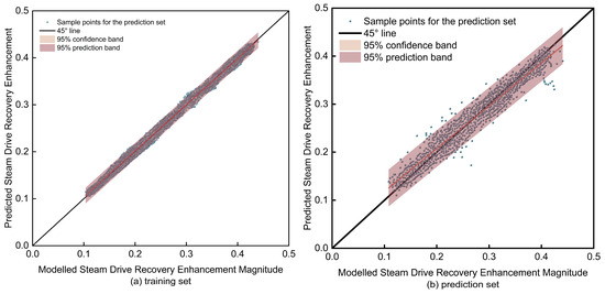
Figure 17.
Scatter plots of the tuned LightGBM predicted vs. actual steam-drive potential: (a) training set; (b) test set.
A further comparison between pure cross-validation and the “cross-validation + random search” optimization approaches shows that, although the latter slightly reduced accuracy on the training set, it significantly improved prediction accuracy on the test set: overall, R2 increased, while RMSE, MAE, and MRE all decreased (see Figure 18). This indicates that random search, while improving optimization efficiency, effectively avoids local optima and suppresses overfitting, further enhancing model generalization. Therefore, the constructed LightGBM model performs outstandingly in terms of prediction accuracy, stability, and efficiency.
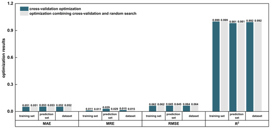
Figure 18.
Evaluation of cross-validation and of cross-validation combined with random search.
3.3. Establishment of the Mathematical Model for Injection–Production Parameter Optimization
3.3.1. Mathematical Model for Optimizing Injection–Production Parameters When Switching to Steam Flooding
In the process of switching from multi-cycle steam stimulation to steam flooding, the reasonable optimization of injection–production parameters is key to improving development performance. The optimization problem consists of three parts: the optimization variables (see Equation (9)), the objective function (see Equation (10)) and the constraints (see Equation (11)). Optimization variables are the development parameters that can be adjusted within allowable ranges; different combinations correspond to different development schemes, and the optimal solution is the one that optimizes the objective function. The objective function measures scheme quality, and can be cumulative incremental oil or economic benefit. Constraints limit the variable ranges to ensure the scheme meets actual production conditions, including upper and lower bounds and equality constraints.
In the equation, is commonly used to denote the constraint functions; denotes the number of constraints.
3.3.2. Mathematical Model for Optimizing Continuous Steam Injection
- (1)
- Optimization variables
For the continuous steam-injection problem when switching to steam flooding after multiple cycles, the main parameters to be optimized include: steam injection rate , steam quality (dryness) , injection temperature , and liquid production rate . For a target reservoir containing injection wells and production wells,
In the equation, is the steam injection rate of the well; is the injected steam quality of the well; is the injection temperature of the well; and is the liquid production rate of the well.
- (2)
- Objective function
The objective function maximizes economic net present value (NPV), taking into account oil revenue and the costs of steam injection and produced water treatment. The NPV objective can be expressed as the difference between increased cash inflows and cash outflows over the production period. In this study, cash inflows are the additional revenue from incremental oil production during the production period, and cash outflows are production costs and produced water treatment costs. The objective function is given by the following formula:
In the equation, and denote the oil and water production, respectively, of well in year (units as given); R is the oil selling price (CNY per unit); is the produced-water treatment cost (CNY·); is the steam-injection cost (CNY·); is the evaluation period (years); is the number of production wells; is the number of injection wells; and is the discount rate, . Except for the production data, all other parameters in the objective function are preset; their values are given in Table 6.
Table 6.
Table of parameter values for economic net present value calculations.
- (3)
- Constraints
The constraints to be considered in the injection optimization problem include: ① upper and lower bounds on steam injection rate; ② upper and lower bounds on injected steam quality; ③ injection temperature constraints; ④ upper and lower bounds on liquid production rate; ⑤ total liquid production constraint for the block; ⑥ total steam injection constraint for the block.
Upper and lower bounds on the steam injection rate refer to the fact that rates that are too low will reduce displacement efficiency, while rates that are too high increase the risk of steam channeling; the mathematical form of this constraint is as follows:
In the equation, denotes the injection well ; and are the minimum and maximum steam injection rates for well , respectively.
Bounds on injected steam quality: The injected steam quality for each injection well should be kept within a reasonable range and must not be too low. The mathematical expression of this constraint is as follows:
In the equation, denotes the injection well ; and are the minimum and maximum injected steam quality for the well, respectively. In injected steam quality optimization, is typically set to 1.
Injection temperature constraint: Too low a temperature will produce a hot water drive, while too high a temperature reduces the heating range. The mathematical expression of this constraint is as follows:
In the equation, denotes the injection well ; and are the minimum and maximum injection temperatures for well I, respectively.
Upper and lower bounds on the liquid production rate prevent capacity being too low or too high. The mathematical expression of this constraint is
where denotes the production well ; and are the minimum and maximum liquid production rates for well I, respectively.
Total block liquid-production constraint: The allocation among wells must satisfy a fixed total liquid production. The mathematical expression of this constraint is
where denotes the production well , is the liquid production of well , and is the total liquid production of the block.
Total block steam-injection constraint: The total steam injected is kept constant, only the distribution among wells is reallocated. The mathematical expression of this constraint is
where denotes the injection well ; is the steam injection volume of well ; and is the total steam injection volume of the block.
Among the above constraints, the ranges for steam injection rate, injected steam quality, injection temperature, and liquid production rate are upper-and-lower-bound constraints (inequality bounds). The block total liquid production and total steam injection are required to remain constant and thus constitute equality constraints.
3.3.3. Mathematical Model for Optimizing Intermittent Steam Injection
- (1)
- Optimization variables
After multiple cycles of huff-and-puff, the field is switched to steam drive and developed using intermittent steam injection,; the optimization variables include steam injection rate , steam quality , injection temperature , injection duration , shut-in duration , and liquid production rate . For a target reservoir containing injection wells and production wells,
where is the steam injection rate of the injection well; is the injection steam quality (dryness) of the injection well; is the injection temperature of the injection well; is the injection duration of the injection well; is the shut-in duration of the injection well; and is the liquid production rate of the production well.
- (2)
- Objective function
Same as the objective function for continuous steam injection.
- (3)
- Constraints
The constraints on steam injection rate , steam quality , injection temperature , and liquid production rate are the same as for the continuous steam injection variables, all implemented as upper and lower bound constraints. For intermittent injection, the reservoir total liquid production and total injected steam are both enforced as equality constraints, consistent with continuous injection.
① Upper and lower bound constraints on injection duration. If too short, heating is insufficient; if too long, the oil-to-gas ratio decreases. The mathematical expression of this constraint is as follows:
In the equation, denotes the steam injection well, ; and are, respectively, the minimum and maximum injection times of the well.
② Upper and lower bound constraints on the shut-in time. If it is too short, the heat is not fully utilized; if it is too long, reheating is insufficient. The total liquid production and the total injected steam must still be kept constant. The mathematical expression of this constraint is as follows:
In the equation, denotes the steam injection well, ; and are, respectively, the minimum and maximum injection times of the well.
3.3.4. Mathematical Model for Optimizing Asynchronous Injection–Production
- (1)
- Optimization variables
When converting to steam flooding after multiple cycles of huff-and-puff and developing by intermittent steam injection, the optimization variables include steam injection rate , injection steam quality , injection temperature , injection time , soak (shut-in) time , production time , and liquid production rate . For a target reservoir containing injection wells and production wells,
In the equation, is the steam injection rate of the injection well; is the injection steam quality of the injection well; is the injection temperature of the injection well; is the injection time of the injection well; is the soak (shut-in) time of the injection well; is the production time of the production well; and is the liquid production rate of the production well.
- (2)
- Objective function
Identical to the objective function for continuous steam injection.
- (3)
- Constraints
The constraints on steam injection rate , injection steam quality , injection temperature , injection time , and liquid production rate are the same as for intermittent steam injection, all implemented as upper and lower bound constraints. In asynchronous injection–production, the reservoir’s total liquid production and total injected steam are enforced by equality constraints, consistent with continuous steam injection.
① Upper and lower bound constraints on soak (shut-in) time. If it is too short, diffusion is insufficient; if it is too long, heat loss increases. The mathematical expression of this constraint is as follows:
In the equation, denotes the steam injection well, ; and are, respectively, the minimum and maximum soak (shut-in) times of the injection well.
② Upper and lower bound constraints on production time. If it is too short, the heat is not fully utilized; if it is too long, the energy is depleted. The mathematical expression of this constraint is as follows:
In the equation, denotes the steam injection well, ; and are, respectively, the minimum and maximum soak (shut-in) times of the injection well.
3.3.5. Mathematical Model for Optimizing First Continuous Injection Then Switching to Intermittent Injection
- (1)
- Optimization variables
Continuous injection followed by intermittent injection is a combined form of the optimization variables for continuous and intermittent injection. Its optimization variables include steam injection rate, injection steam quality, injection temperature, liquid production rate, injection time, and shut-in time; these variables have the same forms as in the continuous and intermittent injection cases. This injection production scheme also includes the switching time Rc1 (the timing of switching to intermittent injection). For a target reservoir containing injection wells and production wells,
In the equation, denotes the time at which the injection well switches from continuous to intermittent injection.
- (2)
- Objective function
Identical to the objective function for continuous steam injection.
- (3)
- Constraints
The constraints for “continuous injection followed by intermittent injection” are basically the same as those for continuous and intermittent injection. The new optimization variable is the switching time from continuous to intermittent injection. It is subject to upper and lower bounds; the switching time for each injection well should be kept within a reasonable range—neither too early nor too late. The mathematical expression of this constraint is as follows:
In the equation, denotes the steam-injection well, ; and are, respectively, the minimum and maximum switching times to intermittent injection for the i injection well. The timing for switching to intermittent injection is measured by the cumulative oil–steam ratio during production, and must not be smaller than the limiting oil–steam ratio, which is typically taken as 0.12.
3.3.6. Mathematical Model for Optimizing First Continuous Injection Then Switching to Asynchronous Injection–Production
- (1)
- The optimization variable “Continuous injection followed by switching to asynchronous injection” is a combination of the two basic schemes—continuous injection and asynchronous injection—so the optimization variables are the merged set of those for continuous and asynchronous injection. The optimization variables for this scheme include steam injection rate, injection steam quality, injection temperature, liquid production rate, injection time, soak (shut-in) time, and production time; these variables have the same forms as in the continuous and asynchronous injection cases.
This injection–production scheme’s optimization variables also include the switching time to asynchronous injection–production. For a target reservoir containing injection wells and production wells,
In the equation, denotes the time at which the injection well switches from continuous injection to asynchronous injection production.
- (2)
- Objective function
Identical to the objective function for continuous steam injection.
- (3)
- Constraints
The constraints for continuous injection followed by intermittent injection are basically the same as those for continuous and intermittent injection; see the sections on continuous and intermittent injection.
For the new optimization variable—the switching time from continuous injection to asynchronous injection production—upper and lower bound constraints are applied, consistent with the switching time constraints for continuous-to-intermittent injection.
3.4. Solution of the Optimization Mathematical Model
The optimization of injection–production parameters for switching to steam flooding after multiple huff-and-puff cycles is characterized by multiple constraints, multimodality (many local optima), and high dimensionality. In this section, based on reservoir numerical simulation methods and intelligent optimization algorithms, a solution approach is proposed to determine the optimal combination of injection–production parameters and thereby optimize the transition to steam flood development.
3.4.1. Bayesian Adaptive Direct Search Algorithm
The optimization of injection–production parameters for steam flooding involves a high-dimensional, nonlinear, and multi-constrained problem in which the objective function—net present value (NPV)—is derived from complex numerical simulations. These characteristics make gradient-based methods inefficient and often prone to local optima. To efficiently explore such complex objective surfaces, this study employs the Bayesian Adaptive Direct Search (BADS) algorithm, an intelligent hybrid optimizer designed for black-box, expensive, or noisy functions.
BADS combines the strengths of Bayesian optimization, which uses probabilistic surrogate models to guide global exploration, and mesh-adaptive direct search, which performs systematic local refinement. During optimization, a Gaussian process surrogate is iteratively updated to model the objective function; an acquisition function selects new candidate points that balance exploitation (searching near current optima) and exploration (sampling uncertain regions). When local convergence stalls, BADS switches to a polling phase that adaptively refines the mesh and adjusts step size, ensuring robustness and convergence toward a global optimum.
Compared with conventional algorithms such as particle swarm optimization (PSO) or CMA-ES, BADS requires fewer function evaluations and is well suited for reservoir optimization problems that couple machine learning surrogates with numerical simulations. Its hybrid search mechanism effectively balances exploration and exploitation, providing both computational efficiency and global reliability. Therefore, BADS is adopted in this work to determine the optimal combination of steam injection rate, quality, temperature, and production rate that maximizes economic NPV across multiple steam flooding scenarios.
3.4.2. Optimization Workflow for Injection Production Parameters When Switching to Steam Flooding After Multiple Huff-and-Puff Cycles
The optimization workflow for injection production parameters when switching to steam flooding after multiple huff-and-puff cycles includes the following steps:
- (1)
- Dynamic numerical simulation of multiple huff-and-puff cycles for the well group. Based on the well-group geological model, reservoir petrophysical parameters, fluid properties, well pattern, and well operating schedules, build a numerical simulation model for multiple huff-and-puff cycles and run dynamic production simulations to output development state data such as temperature, pressure, and saturation fields;
- (2)
- Dynamic numerical simulation of the switch from huff-and-puff to steam flooding for the well group to improve computational efficiency, apply a restart at the final time step of the huff-and-puff simulation and run the model under steam flood operating conditions. Using the previously obtained temperature, pressure, and saturation fields, perform the steam flood dynamic simulation to ensure the continuity and accuracy of the data throughout the optimization;
- (3)
- Optimization of steam flood injection production parameters. Select the BADS algorithm as the optimization method to optimize injection production parameters for the transition to steam flooding after multiple huff-and-puff cycles. Define constraints and initial values and optimize based on the objective function (e.g., net present value). During optimization, couple the BADS algorithm with the numerical simulation model to optimize the injection production parameters, and output the optimal scheme’s injection rates, liquid production rates, cumulative incremental oil, and net present value.
3.5. Validation of the Optimization Mathematical Model
Based on the above solution approach for the optimization model, the five proposed optimization mathematical models were solved. To validate the efficiency and accuracy of the proposed method, computations were performed using the aforementioned heavy oil model, and the machine learning optimization results were compared with orthogonal experimental results from numerical simulation.
3.5.1. Validation of the Optimization Mathematical Model for Continuous
- (1)
- Injection production parameter optimization results
Based on the typical block/typical well location model introduced above, a dynamic production simulation was set up for switching to continuous steam injection after multiple huff-and-puff cycles. The continuous-injection parameter optimization method was used to solve the model’s optimization variables. The model contains six production wells and three injection wells, with a total of 11 optimization variables, including injection rate, liquid production rate, injection temperature, and injection steam quality. The objective function is the economic net present value (NPV) of cumulative incremental oil; the optimization was performed using the BADS algorithm. The optimization results are shown in Figure 19.
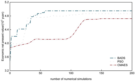
Figure 19.
Optimization dynamics of continuous injection.
Compared with the particle swarm optimization (PSO) and the covariance matrix adaptation evolution strategy (CMA-ES), the BADS algorithm demonstrated superior optimization performance. Within 60 numerical simulations, BADS was able to find the optimal solution, and its results were significantly better than those of the other algorithms. The best solution is injection rates for the three injection wells of 145.5 m3/d, 128.7 m3/d, and 144.6 m3/d; liquid production rates for the six production wells of 100 t/d, 94.1 t/d, 95.3 t/d, etc.; injection temperature 289.9 °C; injection steam quality 0.79. Under this scheme, the cumulative incremental oil is 202,452 tonnes and the economic net present value is CNY 49.51 million.
- (2)
- Results of the orthogonal experiment design
To further validate the optimization method, orthogonal experiments were conducted on the schemes listed in the orthogonal table (Table 7), optimizing four factors: injection rate, liquid production rate, injection steam quality, and injection temperature.
Table 7.
Parameters of the continuous steam-injection optimization model and their values.
In the experimental design shown in Table 8, the four factors were each set at three levels, forming 81 combinations, while the orthogonal experiment required only nine trials to obtain representative data. The test results are shown in Table 3; the optimal scheme’s injection production parameters are injection rate 175 m3/d, injection steam quality 0.85, injection temperature 225 °C, and liquid production rate 201.25 t/d. Under this scheme, the cumulative incremental oil is 176,854 tonnes and the economic net present value is CNY 43.5468 million.
Table 8.
Orthogonal experimental design table for continuous steam-injection optimization.
Figure 20 shows a comparison between the orthogonal experimental design and the optimization method results. Compared with the orthogonal design scheme, the proposed intelligent optimization method increased cumulative incremental oil by 25,598 tonnes (a 14.47% increase) and raised the economic net present value by CNY 5.964 million (a 13.69% increase). These results validate the accuracy of the optimization method and indicate it can effectively improve cumulative incremental oil and NPV.
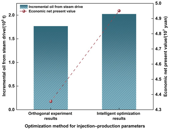
Figure 20.
Comparison of orthogonal experimental design and intelligent optimization results for continuous injection.
Further analyzing the optimization effects, Figure 21 and Figure 22 compare the temperature field and oil saturation field for the orthogonal experimental design and the intelligent optimization method. By differentially allocating injection and production among wells, the optimization method significantly improved steam utilization and sweep efficiency (see Figure 21) and further enhanced development performance (see Figure 22).
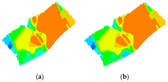
Figure 21.
Comparison of temperature fields of the optimal schemes from orthogonal experimental design and the intelligent optimization method for continuous injection. They should be listed as: (a) Orthogonal experimental design optimization; (b) intelligent optimization method optimization.
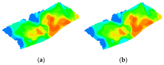
Figure 22.
Comparison of saturation fields of the optimal schemes from the orthogonal experimental design and the intelligent optimization method for continuous injection. They should be listed as: (a) Orthogonal experimental design optimization; (b) intelligent optimization method optimization.
3.5.2. Validation of the Optimization Mathematical Model for Intermittent Steam Injection
- (1)
- Injection production parameter optimization results
For the model that switches to intermittent steam injection after multiple huff-and-puff cycles, the intermittent injection optimization method was used to determine the optimal injection production parameters during development. The model includes six production wells and three injection wells; the optimization variables comprise 13 parameters, including the liquid production rates of the six production wells, the injection rates of the three injection wells, injection time, shut-in (soak) time, injection temperature, and injection steam quality. Using the economic net present value of cumulative incremental oil as the objective function, optimization was performed with the BADS algorithm, yielding the optimal injection–production scheme shown in Figure 23.
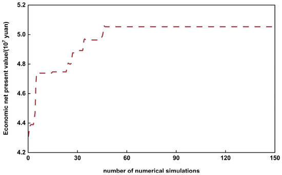
Figure 23.
Optimization dynamics of intermittent injection.
The optimization results show that the BADS algorithm can obtain the optimal value of the objective function in fewer than 60 numerical simulations. The optimal scheme has injection rates of 199.9 m3/d, 193.4 m3/d, and 200 m3/d; liquid production rates for the production wells of 140.1 t/d, 118.9 t/d, 175.2 t/d, etc.; an injection time of 39.7 days; a shut-in time of 13.9 days; an injection temperature of 288.24 °C; and an injection steam quality of 0.75. Under this scheme the cumulative incremental oil is 206,517 tonnes and the economic net present value is CNY 50.6308 million, demonstrating the effectiveness of the optimization method.
- (2)
- Results of the orthogonal experimental design
To further validate the reasonableness of the optimization results, an orthogonal experimental design was used to analyze the optimization parameters for intermittent steam injection. The orthogonal array in Table 9, Table 10 was selected to simulate 25 combination schemes, and the cumulative incremental oil and economic net present value were obtained for each scheme. Table 9 and Table 10 list the optimization variables and their value ranges.
Table 9.
Parameters of the intermittent steam-injection optimization model and their values.
Table 10.
Orthogonal experimental design table for intermittent steam-injection optimization.
The final optimal injection production parameter set is injection rate 225 m3/d, injection steam quality 0.9, injection temperature 250 °C, liquid production rate 258.75 t/d, injection time 20 days, and shut-in time 10 days. Using this parameter set for intermittent injection development yields a cumulative incremental oil of 184,373 tonnes and an economic net present value of CNY 46.4425 million. Compared with the orthogonal experimental design, the intelligent optimization method’s scheme shows higher incremental oil and NPV, with increases of 12.01% and 9.02%, respectively. Figure 24 presents the comparison results, further demonstrating the advantage of the optimization method.
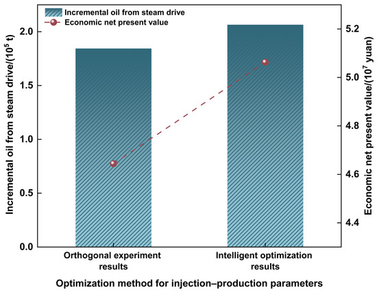
Figure 24.
Comparison of orthogonal experimental design and intelligent optimization results for intermittent steam injection.
Figure 25 and Figure 26 show comparisons of the temperature field and oil saturation field obtained from the orthogonal experimental design and the intelligent optimization method under the optimized scheme. Figure 25 indicates that by differentially allocating injection among wells using the intelligent optimization method, steam utilization and sweep efficiency are significantly improved; Figure 26 shows that the differential allocation of production wells leads to a marked improvement in development performance. This demonstrates that the optimized scheme can effectively enhance steam heat utilization and the sweep efficiency for oil and gas, thereby improving overall reservoir development.
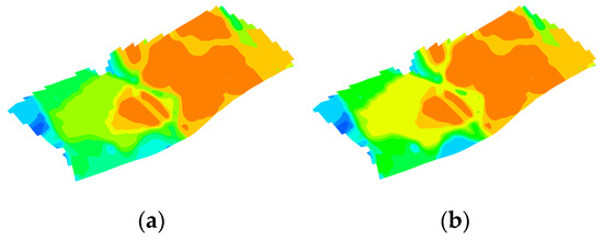
Figure 25.
Comparison of temperature fields of the optimal schemes from the orthogonal experimental design and the intelligent optimization method for intermittent steam injection, which should be listed as: (a) optimization results of the orthogonal experimental design; (b) optimization results of the intelligent optimization method.
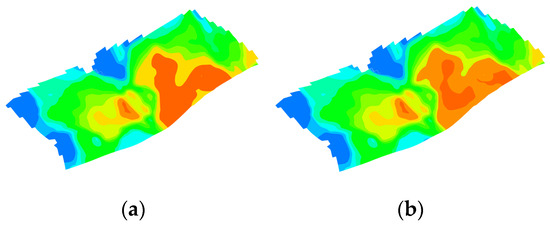
Figure 26.
Comparison of saturation fields of the optimal schemes from the orthogonal experimental design and the intelligent optimization method for intermittent steam injection, which should be listed as: (a) optimization results of the orthogonal experimental design; (b) optimization results of the intelligent optimization method.
3.5.3. Validation of the Optimization Mathematical Model for Asynchronous Injection Production
- (1)
- Injection production parameter optimization results
For the model that switches to asynchronous injection production steam flooding after multiple huff-and-puff cycles, the asynchronous injection production optimization method was used to solve the model’s optimization variables. The model includes six production wells and three injection wells; the optimization variables comprise 14 parameters, including liquid production rates, injection rates, injection time, soak (shut-in) time, production time, injection temperature, and injection steam quality. Using the economic net present value of cumulative incremental oil as the objective function, dynamic optimization was performed with the BADS algorithm. After approximately 120 numerical simulations, the optimal solution was obtained. The optimization results are shown in Figure 27. The optimal injection production scheme is injection rates for the three injection wells of 201.3 m3/d, 196.4 m3/d, and 162.5 m3/d; liquid production rates for the six production wells of 237.0 t/d, 126.6 t/d, etc.; an injection time 22.5 days; a soak time of 1 day; a production time of 41.5 days; an injection temperature of 213.48 °C; and an injection steam quality of 0.82. Under this scheme the cumulative incremental oil is 184,479 tonnes and the economic net present value is CNY 47.6584 million.
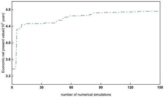
Figure 27.
Optimization dynamics of asynchronous injection–production.
- (2)
- Results of the orthogonal experimental design
The optimization variables for asynchronous injection–production include injection rate, liquid production rate, injection steam quality, injection temperature, injection time, soak (shut-in) time, and production time (see Table 11).
Table 11.
Modeling parameters and their values for asynchronous injection/production optimization.
The optimization variables for asynchronous injection–production include injection rate, liquid production rate, injection steam quality, injection temperature, injection time, soak (shut-in) time, and production time. Orthogonal experiments were performed using orthogonal Table 12 for 18 combination schemes. The results show that when simulated up to an oil–steam ratio of 0.12, the best injection–production parameter set is injection rate 175 m3/d, injection steam quality 0.85, injection temperature 225 °C, liquid production rate 201.25 t/d, injection time 35 days, soak time 3 days, and production time 55 days. Using this optimal combination for asynchronous injection production steam flooding yields a cumulative incremental oil of 158,107 tonnes and an economic net present value of CNY 45.2643 million.
Table 12.
Orthogonal experimental design table for asynchronous injection/production optimization.
By comparing the results of the orthogonal experimental design and the optimization method (see Figure 28), it is evident that the optimization method outperforms the orthogonal design in the transition to steam flood development. Specifically, cumulative incremental oil increased by 26,372 tonnes (a 16.68% rise), and the economic net present value grew by CNY 5.3941 million (a 12.73% rise). These results validate the effectiveness and accuracy of the proposed asynchronous injection–production optimization method, indicating it can deliver both higher NPV and greater incremental oil.
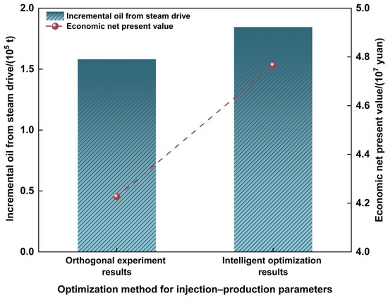
Figure 28.
Comparison of orthogonal experimental design and intelligent optimization results for asynchronous injection production.
To further validate the optimization results, Figure 29 and Figure 30 compare the temperature field and oil saturation field under the optimal schemes from the orthogonal experimental design and the intelligent optimization method. By differentially allocating injection and production among wells using the intelligent optimization method, steam utilization and sweep efficiency were significantly improved. Figure 29 shows that the optimization improved steam injection efficiency, while Figure 30 indicates that differential allocation of production wells further enhanced development performance.
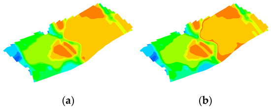
Figure 29.
Comparison of temperature fields of the optimal schemes from the orthogonal experimental design and the intelligent optimization method for asynchronous injection production, which should be listed as: (a) optimization results of the orthogonal experimental design; (b) optimization results of the intelligent optimization method.
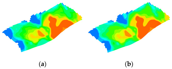
Figure 30.
Comparison of saturation fields of the optimal schemes from the orthogonal experimental design and the intelligent optimization method for asynchronous injection production, which should be listed as: (a) optimization results of the orthogonal experimental design; (b) optimization results of the intelligent optimization method.
3.5.4. Validation of the Optimization Mathematical Model for Continuous Injection Followed by Intermittent Steam Injection
- (1)
- Injection production parameter optimization results
For the model that switches to continuous injection followed by intermittent steam injection after multiple huff-and-puff cycles, the proposed optimization method was used to solve the optimization variables. The model includes six production wells and three injection wells, with a total of 14 optimization variables such as liquid production rates, injection rates, injection time, shut-in time, injection temperature, injection steam quality, and the timing by oil–steam ratio. Using the economic net present value of cumulative incremental oil as the objective function, the problem was solved with the BADS algorithm. After about 120 simulations, the optimal solution was obtained. The optimal injection–production scheme is injection rates for the three injection wells of 82.3 m3/d, 200.0 m3/d, and 193.9 m3/d; liquid production rates for the six production wells of 143.4 t/d, 52.3 t/d, 113.8 t/d, etc.; injection time 60 days; shut-in time 10 days; injection temperature 208.35 °C; injection steam quality 0.72; and oil–steam ratio timing of 0.33. As shown in Figure 31, under this scheme the cumulative incremental oil is 276,032 tonnes and the economic net present value is RMB 49.8985 million.
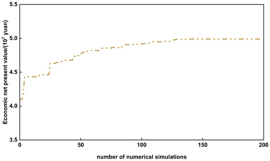
Figure 31.
Optimization dynamics of switching from continuous injection to intermittent injection.
- (2)
- Results of the orthogonal experimental design
The optimization variables for continuous injection followed by intermittent injection include injection rate, liquid production rate, injection steam quality, injection temperature, timing based on the oil–steam ratio, injection time, and shut-in time (see Table 13).
Table 13.
Parameters and their values for the optimization model of continuous injection followed by intermittent injection.
Orthogonal experiments were conducted on 18 combination schemes from the orthogonal table (Table 14), with simulations run until the oil–steam ratio reached 0.12. The results show that the optimal injection–production parameter set is injection rate 175 m3/d, injection steam quality 0.75, injection temperature 325 °C, liquid production rate 201.25 t/d, injection time 45 days, and shut-in time 35 days. Using this parameter set for continuous injection followed by intermittent injection steam flood development yields a cumulative incremental oil of 246,116 tonnes and an economic net present value of CNY 44.3358 million.
Table 14.
Orthogonal experimental design table for optimization of continuous injection followed by intermittent steam injection.
Figure 32 compares the orthogonal experimental design and the optimization method. The scheme found by the optimization method increased the NPV of the transition to steam flooding by CNY 5.563 million (12.55%) and raised cumulative incremental oil by 29,916 tonnes (12.16%) compared with the orthogonal design. These results validate the effectiveness of the proposed optimization method, indicating it can deliver higher NPV and greater incremental production.
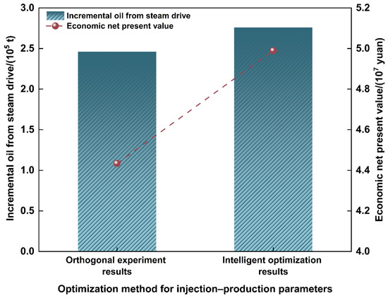
Figure 32.
Comparison of orthogonal experimental design and intelligent optimization results.
To further validate the optimization effects, Figure 33 and Figure 34 compare the temperature field and oil saturation field under the optimal schemes from the orthogonal experimental design and the intelligent optimization method. Differentially allocating injection among wells with the intelligent optimization method significantly improves steam utilization and sweep efficiency (see Figure 33). At the same time, the differential allocation of production wells further enhances development performance (see Figure 34).
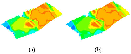
Figure 33.
Comparison of temperature fields of the optimal schemes from the orthogonal experimental design and the intelligent optimization method for continuous injection followed by intermittent injection. (a) Optimization results of the orthogonal experimental design; (b) optimization results of the intelligent optimization method.
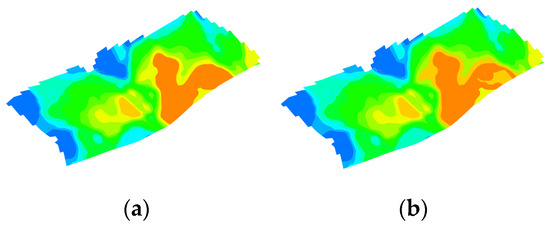
Figure 34.
Comparison of saturation fields of the optimal schemes from the orthogonal experimental design and the intelligent optimization method for continuous injection followed by intermittent injection. (a) Optimization results of the orthogonal experimental design; (b) optimization results of the intelligent optimization method.
3.5.5. Validation of the Optimization Mathematical Model for Continuous Injection Followed by Switching to Asynchronous Injection Production
- (1)
- Injection production parameter optimization results
Based on the model that switches to continuous injection followed by asynchronous injection production after multiple huff-and-puff cycles, the proposed optimization method was used to solve the optimization variables. The model includes six production wells and three injection wells, with a total of 15 optimization variables such as injection rate, liquid production rate, injection time, soak (well shut-in) time, shut-in/off-injection time, production time, injection temperature, injection steam quality, and the oil–steam ratio switching time. Optimization was performed with the BADS algorithm using the economic net present value of cumulative incremental oil as the objective function. The BADS algorithm showed good performance and quickly found the optimum after roughly 120 simulations. The optimal scheme is injection rates of 50.0 m3/d, 88.8 m3/d, and 136.3 m3/d for the three injection wells; liquid production rates of 99.6 t/d, 67.9 t/d, 80.9 t/d, etc., for the six production wells; injection time 60 days; soak time 4 days; production time 15 days; injection temperature 297.56 °C; injection steam quality 0.76; and oil–steam ratio switching time 0.28. Under this scheme, the cumulative incremental oil is 182,512 tonnes and the economic net present value is CNY 48.836 million (see Figure 35).
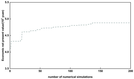
Figure 35.
Optimization dynamics of switching from continuous injection to asynchronous injection production.
- (2)
- In the results of the orthogonal experimental design, the optimization variables for continuous injection followed by switching to asynchronous injection–production include injection rate, liquid production rate, injection steam quality, injection temperature, timing based on the oil–steam ratio, injection time, soak (shut-in) time, and production time (see Table 15).
Table 15. Parameters and their values for the optimization model of continuous injection followed by asynchronous injection/production.
Orthogonal experiments were used to simulate 18 parameter combinations from the design table (Table 16), with simulations stopped when the oil–steam ratio reached 0.12. The optimal injection production parameter set is: injection rate 150 m3/d, injection steam quality 0.8, injection temperature 250 °C, liquid production rate 110 t/d, injection time 40 days, soak time 5 days, production time 50 days, and oil–steam-ratio switching timing 0.25. Using this scheme for steam flood development, the cumulative incremental oil after switching to steam flooding is 165,125 tones, and the economic net present value is CNY 43.665 million.
Table 16.
Orthogonal experimental design table for optimization of continuous injection followed by asynchronous injection/production.
Figure 36 compares the results of the orthogonal experimental design and the optimization method. The scheme found by the optimization method increased NPV by CNY 5.171 million (11.84%) and raised cumulative incremental oil by 17,387 tonnes (10.53%) compared with the orthogonal design. These results validate the efficiency and accuracy of the proposed optimization method, indicating it can deliver higher NPV and greater incremental oil.
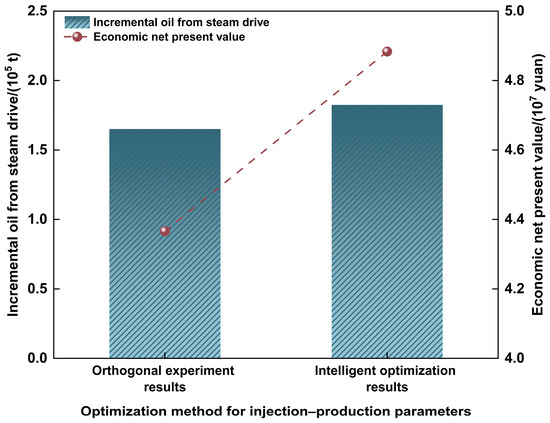
Figure 36.
Comparison of orthogonal experimental design and intelligent optimization results for continuous injection followed by asynchronous injection production.
To further validate the optimization results, Figure 37 and Figure 38 compare the temperature field and oil saturation field from the orthogonal experimental design and the intelligent optimization method. By differentially allocating injection and production wells, the optimization method significantly improves steam utilization and sweep efficiency (see Figure 37). At the same time, the differential allocation of production wells further enhances development performance (see Figure 38).
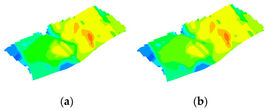
Figure 37.
Comparison of temperature fields of the optimal schemes from the orthogonal experimental design and the intelligent optimization method for continuous injection followed by asynchronous injection production. (a) Optimization results of the orthogonal experimental design; (b) optimization results of the intelligent optimization method.
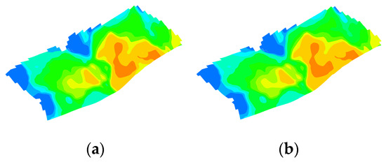
Figure 38.
Comparison of saturation fields of the optimal schemes from the orthogonal experimental design and the intelligent optimization method for continuous injection followed by asynchronous injection–production. (a) Optimization results of the orthogonal experimental design; (b) optimization results of the intelligent optimization method.
4. Conclusions
- (1)
- A numerical simulation model was developed for well groups switching to steam flooding after multiple huff-and-puff cycles, comprehensively accounting for the effects of temperature on rock thermal properties, the viscosity–temperature relationship, and relative permeability curves. The model can accurately reflect actual production dynamics;
- (2)
- Based on single-factor and multi-factor analyses, the key factors affecting steam flood potential were identified, including remaining reserves at the time of implementation, effective reservoir thickness, coefficient of variation of permeability, water cut, formation temperature, formation pressure, degree of depletion, and well spacing—providing a basis for parameter sensitivity evaluation;
- (3)
- By building many conceptual models with different parameter combinations and running numerical simulations to generate training samples (using the incremental increase in steam flood recovery as the output), predictive models were trained using artificial neural networks, GBDT, XGBoost, and LightGBM. LightGBM performed best. After optimization, the correlation coefficient R2 between predicted and actual values reached 0.991, demonstrating this method’s advantages in prediction accuracy and efficiency and its potential to replace traditional numerical simulation for rapid prediction;
- (4)
- This study used economic net present value maximization as the objective function to establish injection–production optimization models for continuous injection, intermittent injection, asynchronous injection production, and their combinations, and solved them with the BADS algorithm. The optimized schemes achieved higher economic benefits and greater cumulative incremental oil compared with orthogonal experiment results, providing effective methods and technical support for predicting steam flood potential and optimizing injection production in heavy oil reservoirs.
Author Contributions
Conceptualization, L.J. and G.S.; methodology, X.L.; software, S.L.; validation, M.L. and J.L. All authors have read and agreed to the published version of the manuscript.
Funding
This research was funded by Tianshan Elite Talent Cultivation Program, grant number 2022TSYCJC0032.
Data Availability Statement
The datasets presented in this article are not readily available because [the data used in this article originate from an on-site field project that has not yet been concluded, the simulation data are not being publicly shared at this time. We will consider making them publicly available in subsequent work once the project is completed].
Conflicts of Interest
Authors Lu Jia, Guowei Shi, Xing Lu, SiXu Li, Mingju Lan and Junhao Li were employed by the Digital Intelligent Technology Company, Xinjiang Oilfield Branch, Fengcheng Oil Production Plant, Xinjiang Oilfield Branch. The authors declare that the research was conducted in the absence of any commercial or financial relationships that could be construed as a potential conflict of interest.
References
- Tong, X.; Zhang, G.; Wang, Z.; Wen, Z.; Tian, Z.; Wang, H.; Ma, F.; Wu, Y. Distribution and Potential of Global Oil and Gas Resources. Pet. Explor. Dev. 2018, 45, 779–789. [Google Scholar] [CrossRef]
- Zou, C.; Zhai, G.; Zhang, G.; Wang, H.; Zhang, G.; Li, J.; Wang, Z.; Wen, Z.; Ma, F.; Liang, Y.; et al. Formation, Distribution, Potential and Prediction of Global Conventional and Unconventional Hydrocarbon Resources. Pet. Explor. Dev. 2015, 42, 14–28. [Google Scholar] [CrossRef]
- Sun, Q.; Zhang, N.; Liu, W.; Li, B.; Li, S.; Bhusal, A.; Wang, S.; Li, Z. Insights into Enhanced Oil Recovery by Thermochemical Fluid Flooding for Ultra-Heavy Reservoirs: An Experimental Study. Fuel 2023, 331, 125651. [Google Scholar] [CrossRef]
- Temizel, C.; Canbaz, C.H.; Tran, M.; Abdelfatah, E.; Jia, B.; Putra, D.; Irani, M.; Alkouh, A. A Comprehensive Review Heavy Oil Reservoirs, Latest Techniques, Discoveries, Technologies and Applications in the Oil and Gas Industry. In Proceedings of the SPE International Heavy Oil Conference and Exhibition, Kuwait City, Kuwait, 10–12 December 2018. [Google Scholar]
- Pan, Y.; Qiao, W.; Chi, D.; Li, Z.; Shu, Y. Research of Steam Injection In-Situ Production Technology to Enhance Unconventional Oil and Gas Recovery: A Review. J. Anal. Appl. Pyrolysis 2024, 177, 106332. [Google Scholar] [CrossRef]
- Yan, X.; Pang, Z.; Liu, D.; Wang, B. The Characteristics of Steam Chamber Expanding and the EOR Mechanisms of Tridimensional Steam Flooding (TSF) in Thick Heavy Oil Reservoirs. Geoenergy Sci. Eng. 2025, 244, 213434. [Google Scholar] [CrossRef]
- Pang, Z.; Wang, L.; Yin, F.; Lyu, X. Steam Chamber Expanding Processes and Bottom Water Invading Characteristics during Steam Flooding in Heavy Oil Reservoirs. Energy 2021, 234, 121214. [Google Scholar] [CrossRef]
- Xu, A.; Mu, L.; Fan, Z.; Wu, X.; Zhao, L.; Bo, B.; Xu, T. Mechanism of Heavy Oil Recovery by Cyclic Superheated Steam Stimulation. J. Pet. Sci. Eng. 2013, 111, 197–207. [Google Scholar] [CrossRef]
- Kovscek, A.R. Emerging Challenges and Potential Futures for Thermally Enhanced Oil Recovery. J. Pet. Sci. Eng. 2012, 98, 130–143. [Google Scholar] [CrossRef]
- Wu, Z.; Liu, H. Investigation of Hot-Water Flooding after Steam Injection to Improve Oil Recovery in Thin Heavy-Oil Reservoir. J. Pet. Explor. Prod. Technol. 2019, 9, 1547–1554. [Google Scholar] [CrossRef]
- Bao, Y.; Wang, J.; Gates, I.D. On the Physics of Cyclic Steam Stimulation. Energy 2016, 115, 969–985. [Google Scholar] [CrossRef]
- Wang, Y.; Zhang, L.; Deng, J.; Wang, Y.; Ren, S.; Hu, C. An Innovative Air Assisted Cyclic Steam Stimulation Technique for Enhanced Heavy Oil Recovery. J. Pet. Sci. Eng. 2017, 151, 254–263. [Google Scholar] [CrossRef]
- Guevara, J.L.; Patel, R.G.; Trivedi, J.J. Optimization of Steam Injection for Heavy Oil Reservoirs Using Reinforcement Learning. In Proceedings of the SPE International Heavy Oil Conference and Exhibition, Kuwait City, Kuwait, 10–12 December 2018; p. D022S030R002. [Google Scholar]
- Panjalizadeh, H.; Alizadeh, N.; Mashhadi, H. A Workflow for Risk Analysis and Optimization of Steam Flooding Scenario Using Static and Dynamic Proxy Models. J. Pet. Sci. Eng. 2014, 121, 78–86. [Google Scholar] [CrossRef]
- Zhang, R.; Datta-Gupta, A.; Park, J.; Nunna, K.; Briz, E.; Gordillo, R.; Chen, H. Multi-Stage Three-Phase and Compositional History Matching: Field Application to CO2 Enhanced Oil Recovery in the Permian Basin, Texas. Fuel 2025, 387, 134339. [Google Scholar] [CrossRef]
- Yang, S.; Nie, Z.; Wu, S.; Li, Z.; Wang, B.; Wu, W.; Chen, Z. A Critical Review of Reservoir Simulation Applications in Key Thermal Recovery Processes: Lessons, Opportunities, and Challenges. Energy Fuels 2021, 35, 7387–7405. [Google Scholar] [CrossRef]
- Zhang, L.; Xu, C.; Zhang, K.; Yao, C.; Yang, Y.; Yao, J. Production Optimization for Alternated Separate-Layer Water Injection in Complex Fault Reservoirs. J. Pet. Sci. Eng. 2020, 193, 107409. [Google Scholar] [CrossRef]
- Liu, P.; Zheng, H.; Wu, G. Experimental Study and Application of Steam Flooding for Horizontal Well in Ultraheavy Oil Reservoirs. J. Energy Resour. Technol. 2016, 139, 012908. [Google Scholar] [CrossRef]
- Suhag, A.; Ranjith, R.; Balaji, K.; Peksaglam, Z.; Malik, V.; Zhang, M.; Biopharm, F.; Putra, D.; Energy, R.; Wijaya, Z.; et al. Optimization of Steamflooding Heavy Oil Reservoirs. In Proceedings of the SPE Western Regional Meeting, Bakersfield, CA, USA, 23–27 April 2017; SPE: Bakersfield, CA, USA, 2017; p. D041S014R005. [Google Scholar]
- Xi, C.; Qi, Z.; Zhang, Y.; Liu, T.; Shen, D.; Mu, H.; Dong, H.; Li, X.; Jiang, Y.; Wang, H. CO2 Assisted Steam Flooding in Late Steam Flooding in Heavy Oil Reservoirs. Pet. Explor. Dev. 2019, 46, 1242–1250. [Google Scholar] [CrossRef]
- Zhao, D.W.; Wang, J.; Gates, I.D. Optimized Solvent-Aided Steam-Flooding Strategy for Recovery of Thin Heavy Oil Reservoirs. Fuel 2013, 112, 50–59. [Google Scholar] [CrossRef]
- Elbaloula, H.A.; Jin’e, C.; Zichang, T.; Yu, W.; Abdelmajeed, M.; Hamd, M.F. Feasibility Study and Numerical Simulation to Design the Steam Flooding Pilot Test Patterns. J. Pet. Explor. Prod. Technol. 2020, 10, 2559–2573. [Google Scholar] [CrossRef]
- Zhao, Y. Laboratory Experiment and Field Application of High Pressure and High Quality Steam Flooding. J. Pet. Sci. Eng. 2020, 189, 107016. [Google Scholar] [CrossRef]
- Shutler, N.D. Numerical Three-Phase Model of the Two-Dimensional Steamflood Process. Soc. Pet. Eng. J. 1970, 10, 405–417. [Google Scholar] [CrossRef]
- Corsano, A. A Three-Phase, Experimental and Numerical Simulation Study of the Steam Flood Process. In Proceedings of the SPE Annual Technical Conference and Exhibition, New Orleans, LA, USA, 3–6 October 1971. [Google Scholar]
- Coats, K.H.; George, W.D.; Chu, C.; Marcum, B.E. Three-Dimensional Simulation of Steamflooding. Soc. Pet. Eng. J. 1974, 14, 573–592. [Google Scholar] [CrossRef]
- Farouq Ali, S.M.; Ferrer, J. State-of-the-Art of Thermal Recovery Models. J. Energy Resour. Technol. 1981, 103, 296–300. [Google Scholar] [CrossRef]
- Coats, K.H. Simulation of Steamflooding with Distillation and Solution Gas. Soc. Pet. Eng. J. 1976, 16, 235–247. [Google Scholar] [CrossRef]
- Corsano, A.; Sumnu, M.D.; Brigham, W.E.; Aziz, K.; Castanier, L.M. An Experimental and Numerical Study on Steam Injection in Fractured Systems. In Proceedings of the SPE Improved Oil Recovery Conference, Tulsa, OK, USA, 21–24 April 1996. [Google Scholar]
- Mollaei, A.; Maini, B. Steam Flooding of Naturally Fractured Reservoirs: Basic Concepts and Recovery Mechanisms. J. Can. Pet. Technol. 2010, 49, 65–70. [Google Scholar] [CrossRef]
- Souraki, Y.; Ashrafi, M.; Karimaie, H.; Torsæter, O. Experimental Investigation and Numerical Simulation of Steam Flooding in Heavy Oil Fractured Reservoir. In Proceedings of the SPE Western North American Region Meeting, Anchorage, AK, USA, 7–11 May 2011; SPE: Anchorage, AK, USA, 2011; p. SPE-144552-MS. [Google Scholar]
- Saggie-Wexler, K.; Keinan, A.; Ruppin, E. Neural Processing of Counting in Evolved Spiking and McCulloch-Pitts Agents. Artif. Life 2006, 12, 1–16. [Google Scholar] [CrossRef]
- Ali, H.; Muthudoss, P.; Chauhan, C.; Kaliappan, I.; Kumar, D.; Paudel, A.; Ramasamy, G. Machine Learning-Enabled NIR Spectroscopy. Part 3: Hyperparameter by Design (HyD) Based ANN-MLP Optimization, Model Generalizability, and Model Transferability. AAPS PharmSciTech 2023, 24, 254. [Google Scholar] [CrossRef]
- Ikonomovska, E.; Gama, J.; Džeroski, S. Learning Model Trees from Evolving Data Streams. Data Min. Knowl. Discov. 2011, 23, 128–168. [Google Scholar] [CrossRef]
- Farid, D.M.; Zhang, L.; Rahman, C.M.; Hossain, M.A.; Strachan, R. Hybrid Decision Tree and Naïve Bayes Classifiers for Multi-Class Classification Tasks. Expert Syst. Appl. 2014, 41, 1937–1946. [Google Scholar] [CrossRef]
- Hajihosseinlou, M.; Maghsoudi, A.; Ghezelbash, R. A Novel Scheme for Mapping of MVT-Type Pb–Zn Prospectivity: LightGBM, a Highly Efficient Gradient Boosting Decision Tree Machine Learning Algorithm. Nat. Resour. Res. 2023, 32, 2417–2438. [Google Scholar] [CrossRef]
- Zhang, M.; Wang, X.; Chen, C.; Ding, J.; Zhou, X.; Qu, J. Interpretable Ore Classification Using SHAP-Enhanced LightGBM: A Case Study from the Qiaomaishan Deposit, China. Appl. Comput. Geosci. 2025, 28, 100295. [Google Scholar] [CrossRef]
- Wu, D.; Xu, S.; Liu, H.; Guo, P. Sample Unbalanced HRRP Ground Target Recognition Based on Improved Lightgbm. Digit. Signal Process. 2025, 168, 105624. [Google Scholar] [CrossRef]
- Gu, Y.; Yang, Y.; Gao, Y.; Yan, S.; Zhang, D.; Zhang, C. Data-Driven Estimation for Permeability of Simplex Pore-Throat Reservoirs via an Improved Light Gradient Boosting Machine: A Demonstration of Sand-Mud Profile, Ordos Basin, Northern China. J. Pet. Sci. Eng. 2022, 217, 110909. [Google Scholar] [CrossRef]


Disclaimer/Publisher’s Note: The statements, opinions and data contained in all publications are solely those of the individual author(s) and contributor(s) and not of MDPI and/or the editor(s). MDPI and/or the editor(s) disclaim responsibility for any injury to people or property resulting from any ideas, methods, instructions or products referred to in the content. |
© 2025 by the authors. Licensee MDPI, Basel, Switzerland. This article is an open access article distributed under the terms and conditions of the Creative Commons Attribution (CC BY) license (https://creativecommons.org/licenses/by/4.0/).