Data-Driven Sidetrack Well Placement Optimization

Abstract

Sidetracking technology has become a relatively mature approach for redeveloping mature fields and restoring the productivity of old wells. However, the design of conventional sidetracking projects has largely relied on expert experience or numerical simulation, methods that are often time-consuming, labor-intensive, and subjective. To overcome these limitations, this study proposes a data-driven optimization framework for sidetrack well placement. It utilizes machine learning techniques trained on a large-scale synthetic dataset generated from field-informed numerical simulations, to establish a robust machine-learning proxy model. Four predictive models—Linear Regression, Polynomial Regression, Random Forest, and a Backpropagation (BP) Neural Network—were systematically compared, among which the Random Forest model achieved the best predictive accuracy. After hyperparameter optimization, a robust prediction model for sidetracking performance was established, achieving a Mean Squared Error (MSE) of 0.0008 (Root Mean Squared Error, RMSE, of 0.0283) and an R² of 0.8059 on the test set. To further optimize well placement, a mathematical model was formulated with the objective of maximizing the production enhancement rate. Three optimization algorithms—the Multi-Level Coordinate Search (MCS), Differential Evolution (DE), and Covariance Matrix Adaptation Evolution Strategy (CMA-ES)—were evaluated, with the DE algorithm demonstrating superior performance. By integrating the optimized Random Forest predictor with the DE optimizer, a systematic methodology for sidetrack well placement optimization was developed. A field case study validated the approach, showing significant improvements, including a reduced water cut and an incremental cumulative oil production of 82.7 tons. This research demonstrates the simulation-based feasibility of intelligent sidetrack well placement optimization and provides practical guidance for future sidetracking development strategies.

1. Introduction

In the process of oilfield development, the underground oil–water relationship becomes increasingly complex, making it more difficult to exploit remaining oil reserves. Consequently, the number of low-yield and low-efficiency wells continues to rise. Among various enhanced oil recovery (EOR) techniques, sidetracking has emerged as one of the most effective approaches to rejuvenate mature wells and improve overall recovery efficiency [1,2,3]. Other advanced stimulation techniques, such as CO² pre-fracturing, are also central to redevelopment efforts, though their success is highly dependent on specific geological and fluid characteristics [4]. However, designing an optimal sidetrack scheme is a challenging task due to the large number of geological, engineering, and operational factors that must be considered. Traditionally, sidetrack well placement has relied heavily on expert experience and reservoir numerical simulation [5,6]. These approaches, though valuable, are time-consuming, labor-intensive, and highly subjective, which limits their scalability and automation potential in modern field applications.

With the rapid advancement of big data and data science, a new scientific paradigm has emerged—one that leverages data-driven discovery to uncover hidden patterns and construct predictive models for complex systems. This paradigm, often referred to as the “fourth paradigm of science,” complements experimental, theoretical, and simulation-based approaches by offering a new route to insight through data analytics and machine learning [7,8]. In the petroleum industry, this paradigm shift has opened new opportunities for data-driven decision-making and intelligent optimization in drilling, production, and reservoir management. Thus, incorporating machine learning (ML) and artificial intelligence (AI) techniques into sidetrack well design holds significant potential to learn from historical data and expert knowledge, and to provide scientific guidance for future sidetracking decisions.

The main contributions of this study are not to propose a new machine learning algorithm, but rather: (1) To be the first to systematically develop and validate an integrated data-driven framework specifically for the sidetrack well placement optimization problem. (2) To establish a rigorous and automated workflow that combines numerical simulation, Latin Hypercube Sampling, and orthogonal experimental design to generate a high-quality synthetic sidetracking dataset, addressing the critical bottleneck of sparse and unreliable real-world data in this domain.

The remainder of this paper is organized as follows. Section 2 reviews the related work in traditional sidetracking methods and data-driven approaches. Section 3 presents the preparation of the sidetrack well dataset. Section 4 describes the proposed data-driven prediction models for sidetrack performance. Section 5 introduces the optimization framework and its mathematical formulation. Section 6 demonstrates a practical case study, and Section 7 concludes the paper and provides prospects for future research.

2. Related Work

2.1. Traditional Sidetracking Optimization Methods

Traditional sidetrack design approaches are mainly based on expert judgment and reservoir numerical simulation. Expert-driven methods rely on the qualitative or semi-quantitative assessment of reservoir characteristics by geologists and reservoir engineers, including remaining oil distribution, reservoir heterogeneity, and oil–water connectivity. Some studies have attempted to formalize this expert knowledge into scoring systems or rule-based expert models to support sidetrack planning [9]. However, the effectiveness of such approaches is inherently limited by individual expertise and site-specific experience, making them difficult to generalize across different reservoirs.

Numerical simulation offers a more quantitative but still computationally demanding alternative. Engineers typically construct geological and numerical models of the target reservoir, manually define several possible sidetrack trajectories and layers, and then simulate each case to compare performance indicators such as cumulative oil recovery and water-cut reduction. As Magizov et al. [5] pointed out, this process essentially constitutes a constrained scenario analysis rather than a true global optimization. The major bottleneck lies in the enormous computational workload and limited efficiency—practical sidetrack optimization often involves tens of thousands of possible combinations, making exhaustive simulation infeasible. Although reservoir simulation remains indispensable for risk assessment and design validation, it still relies on expert intervention and experience to handle the complex coupling of geological and operational factors [6].

2.2. Data-Driven Approaches in Conventional Well Development

Sidetrack wells share strong geological and engineering similarities with conventional wells; therefore, research progress in data-driven modeling and optimization for conventional wells offers valuable insights for sidetrack design. In recent years, the application of AI and ML techniques in production forecasting and well placement optimization has achieved remarkable success. For production forecasting, Lu et al. [10] developed a hybrid model combining ML and Particle Swarm Optimization (PSO) to predict shale oil production and optimize fracturing parameters, achieving high prediction accuracy. Ojedapo et al. [11] established ARIMA and Holt–Winters statistical models for production prediction, demonstrating excellent short-term forecasting performance. Makhotin [12] applied ML algorithms to evaluate waterflooding efficiency and to guide reservoir ranking and injection optimization. In well placement optimization, AI-based algorithms have been widely investigated. Cullick et al. [13] constructed a multi-constraint optimization model incorporating key reservoir parameters such as porosity and permeability. Mudhafer et al. [14] integrated a Genetic Algorithm (GA) with reservoir simulation to optimize the number and locations of infill wells. Mohammed [15] verified the enhanced optimization efficiency of intelligent algorithms through field implementation, while Du et al. [16] proposed an ensemble-learning-based proxy model framework to further improve production optimization efficiency. These studies collectively demonstrate that combining predictive modeling with intelligent optimization has become a mainstream trend in oilfield development.

Indeed, this trend has intensified in recent research, with numerous studies combining various machine learning surrogates with evolutionary algorithms to solve complex well placement and operational problems. For example, recent studies have applied deep learning proxies like hybrid CNN-GRU models with genetic algorithms to optimize geothermal well placement under geological uncertainty [17], and used Deep Neural Networks to determine the optimal well spacing for underground hydrogen storage in saline aquifers [18]. In the context of CO₂ storage, optimization frameworks have been developed using mixed-integer linear programming (MILP) to guide sink well placement [19], while Musayev et al. [20] integrated an Artificial Neural Network (ANN) with a genetic algorithm (GA) to optimize CO₂ injection and brine production wells. This data-driven optimization approach extends beyond just well placement to include well operations, such as using Transformer-LSTM models to co-optimize well schedules and conformance control parameters [21]. Other recent works have focused on using ML for optimizing complex horizontal well trajectories [22], developing adaptive, constraint-guided evolutionary algorithms enhanced by surrogates [23], or using Graph Network Surrogate Models (GNSM) with differential evolution (DE) algorithms for injector placement [24].

However, existing research remains primarily focused on conventional wells, and intelligent optimization methods tailored to sidetrack wells are still limited. Sidetracking decisions have different constraints and data characteristics (e.g., reliance on an existing wellbore, goal of restoring production in mature fields rather than greenfield development), which means that models from conventional well placement optimization cannot be directly applied. This research gap serves as the fundamental motivation of this study.

2.3. Key Technologies for the Data-Driven Optimization Framework

To address the aforementioned gap, developing an intelligent optimization framework for sidetrack well placement requires the integration of three essential components: data generation, predictive modeling, and optimization algorithm design.

(1) Data generation.

Field data related to sidetrack operations are typically sparse, inconsistent, and incomplete, making them insufficient for reliable ML model training. As a result, numerical simulation has become an effective means of producing large-scale, high-quality synthetic datasets. Techniques such as Latin Hypercube Sampling (LHS) and orthogonal experimental design are widely used to explore multidimensional parameter spaces efficiently with limited simulation runs [25,26]. These techniques form the methodological foundation of the dataset construction adopted in this study.

(2) Predictive modeling.

In reservoir engineering, simple regression models (e.g., linear and polynomial regression) are easy to interpret but inadequate for capturing the nonlinearities inherent in reservoir behavior. Ensemble learning methods such as Random Forest (RF) provide higher robustness and accuracy when dealing with high-dimensional noisy data and have been widely applied in production forecasting and parameter inversion tasks. Therefore, the RF model is selected as the core predictive framework in this study, with comparative evaluation against the Backpropagation (BP) neural network to ensure prediction reliability.

(3) Optimization algorithm design.

Well placement optimization is a nonlinear, high-dimensional, and multi-constrained problem. Traditional gradient-based algorithms are prone to local minima, leading to the increasing use of metaheuristic algorithms such as GA, PSO, and Differential Evolution (DE) [13,14]. Among them, DE achieves an effective balance between global exploration and convergence speed, while Covariance Matrix Adaptation Evolution Strategy (CMA-ES) and Multilevel Coordinate Search (MCS) algorithms have also demonstrated strong robustness in complex engineering optimizations. This study systematically compares these algorithms to identify the most efficient solver for sidetrack optimization. By integrating machine learning–based prediction models with global optimization algorithms, the proposed framework establishes a comprehensive and efficient data-driven approach to intelligent sidetrack well placement.

3. Preparation of the Data Sample Set for Sidetrack Well Placement Design

3.1. Establishing the Indicator System

A sidetrack well is associated with numerous data metrics. This study focuses specifically on those that influence the well’s development performance. Considering a large number of irrelevant metrics would, on the one hand, result in a high workload and significant computational demands, resulting in the “curse of dimensionality.” On the other hand, irrelevant numerical indicators could generate significant noise and interference, potentially leading to inaccurate data mining results. Therefore, it is necessary to establish a scientific framework of indicators to exclude non-essential features and decrease computational demands, while still preserving the key characteristic metrics.

Based on actual field conditions, and by systematically reviewing the parameters involved in sidetracking project design documents, a data indicator system for sidetracking design was formulated by integrating expert experience with reservoir engineering theory. This system comprises three main categories: parameters for reservoir geology, parameters for sidetracking design, and the parameter for sidetracking performance. The reservoir geological parameters include 19 indicators: Permeability, Recovery Factor, Well Drainage Area, Remaining Recoverable Reserves, Initial Water Cut, Average Water Cut, Field-wide Average Permeability, Porosity, Field-wide Average Porosity, Effective Thickness, Field-wide Total Effective Thickness, Oil Saturation at Target, Oil Saturation at Well Location, Coefficient of Variation for Permeability, Coefficient of Variation for Porosity, Coefficient of Variation for Effective Thickness, Permeability Grade Difference, Porosity Grade Difference, and Effective Thickness Grade Difference. The sidetracking design parameters include six indicators: Distance between the new sidetrack and the original wellbore, Injector-Producer Well Spacing, Target Location, Sidetrack X-Coordinate, Sidetrack Y-Coordinate, and Sidetracking Timing. The sidetracking performance parameter includes one indicator: Production Enhancement Rate.

3.2. Preparation of the Sample Dataset

An analysis of the evaluation criteria shows that the success of a sidetracking project is influenced by many factors. In practice, however, oilfield operations present significant constraints. Historical field data is highly fragmented, being stored across disparate sources. Furthermore, the data that can be gathered from sidetracking proposals in various fields fails to comprehensively match the required metrics and is plagued by extensive missing values and outliers.

The sample dataset is the essential foundation for the AI-based algorithm for optimizing sidetrack well placement; therefore, its quality is a prerequisite for this research. The data must be standardized. Assembling a dataset from the available field data that strictly adheres to our evaluation framework would yield a dataset of insufficient quality for this study.

To address this issue, we have chosen to ensure dataset integrity by using numerical simulation to build multiple conceptual models, which in turn generate a large, complete set of synthetic data. This methodology is also scalable; in the future, if high-quality field data becomes available, it can be used to expand the dataset and be applied within the framework developed here.

3.2.1. Modeling Scenario Design

Based on the actual production data from existing sidetracked wells and the corresponding numerical simulation models of the reservoir blocks, this paper extracts and analyzes common features from the collected data to provide theoretical guidance for the design of the conceptual models.

The key to building a conceptual model is to define its structural parameters, such as the number of layers, the number and size of grid blocks, and grid block thickness. Concurrently, it is necessary to define the petrophysical properties for each layer, including parameters such as permeability and porosity. A schematic flowchart illustrates the specific design process for the modeling is shown in Figure 1.

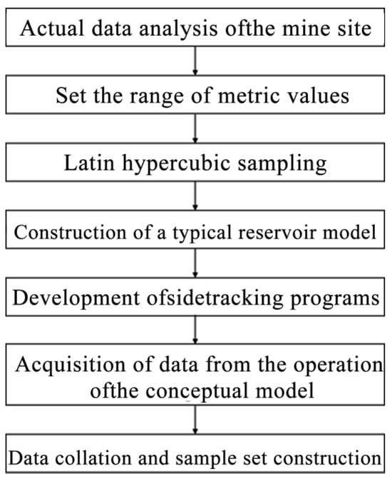
Figure 1. Flowchart for the design of conceptual models for numerical simulation.

The value ranges for each indicator were determined by referencing the collected and compiled field data from actual sidetracking operations. The specific model parameters modified include permeability, porosity, grid block thickness, and grid block size. The specific range for each indicator is shown in Table 1.

Table 1. Value ranges for key parameters of the conceptual models.

Indicator Name	Value Range
Permeability	200–6000 (mD)
Porosity	0.2–0.5
Effective Thickness	0.2–3 (m)
Grid Length/Width	0.2–3 (m)

Within the specified ranges for the key parameters required for the conceptual model design, a full factorial combination of all parameters would generate an excessive number of modeling scenarios. Therefore, this study utilizes Latin Hypercube Sampling (LHS) [25] to generate 500 sets of data samples according to the ranges given in Table 1. Every five sample sets are used to define a conceptual model for one simulated reservoir block, resulting in the creation of 100 initial modeling scenarios. A portion of this data is shown in Table 2. It should be noted that the grid blocks in the conceptual models are square (i.e., equal in length and width). Each sample set represents the parameter data for one layer of the block model, and the grid dimensions for each layer are 51 × 51.

Table 2. Latin hypercube sampling data (partial).

Permeability	Porosity	Grid Thickness (m)	Grid Length (m)	Layer Number	Model Name
4878.535	0.449	0.499	8.084	1	Model 1
527.938	0.495	0.580	6.862	2	Model 1
2861.127	0.212	2.246	7.262	3	Model 1
5013.696	0.318	0.920	9.797	4	Model 1
1959.271	0.258	2.125	4.731	5	Model 1
1548.168	0.407	2.607	9.706	1	Model 2
5875.064	0.235	1.851	10.624	2	Model 2
1855.819	0.442	2.721	10.566	3	Model 2
5426.663	0.477	1.050	3.709	4	Model 2
580.033	0.272	2.058	7.477	5	Model 2

As indicated previously, each reservoir block model initially consists of five reservoir layers. To define the “target location” with greater precision, each of these primary reservoir layers was further subdivided vertically into five sublayers of equal effective thickness. Taking the initial conceptual model as shown in Figure 2 as an example, this vertical refinement results in a new conceptual model with an expanded number of layers, as shown in Figure 3. Consequently, the model is transformed into a conceptual model that comprises 25 discrete reservoir layers in the vertical direction. Different colors are used only to distinguish the grid blocks; they carry no specific physical meaning.

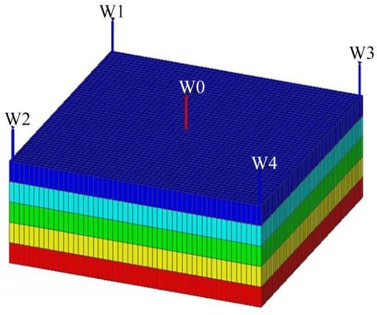
Figure 2. Three-dimensional geological structure of the initial five-layer conceptual model.

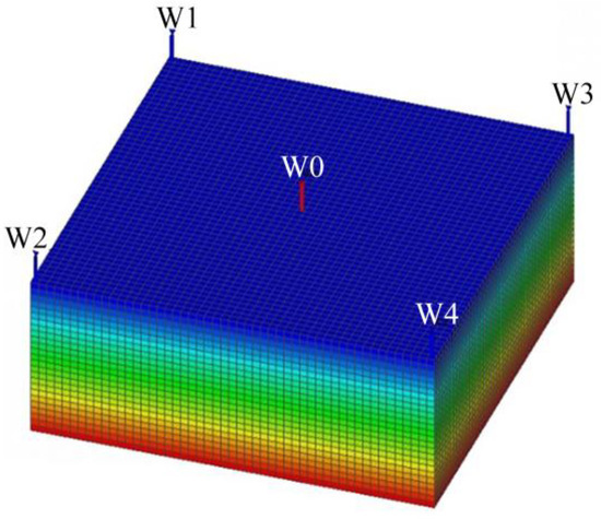
Figure 3. Three-dimensional geological structure of the 25-layer conceptual model after vertical refinement.

Taking Model 1 from Table 2 as an example, the basic parameters for this reservoir block model are listed below in Table 3.

Table 3. Detailed layer parameters for Model 1 (Block 1) after refinement.

Number of Perforated Layers	Permeability	Porosity	Effective Thickness (m)	Grid Length (m)	Target Location
1-1	4878.535	0.449	0.099	8.084	1/5
1-2	4878.535	0.449	0.099	8.084	2/5
1-3	4878.535	0.449	0.099	8.084	3/5
1-4	4878.535	0.449	0.099	8.084	4/5
1-5	4878.535	0.449	0.099	8.084	5/5
2-1	527.938	0.495	0.116	6.862	1/5
2-2	527.938	0.495	0.116	6.862	2/5
2-3	527.938	0.495	0.116	6.862	3/5
2-4	527.938	0.495	0.116	6.862	4/5
2-5	527.938	0.495	0.116	6.862	5/5
3-1	2861.127	0.212	0.449	7.262	1/5
3-2	2861.127	0.212	0.449	7.262	2/5
3-3	2861.127	0.212	0.449	7.262	3/5
3-4	2861.127	0.212	0.449	7.262	4/5
3-5	2861.127	0.212	0.449	7.262	5/5
4-1	5013.696	0.318	0.184	9.797	1/5
4-2	5013.696	0.318	0.184	9.797	2/5
4-3	5013.696	0.318	0.184	9.797	3/5
4-4	5013.696	0.318	0.184	9.797	4/5
4-5	5013.696	0.318	0.184	9.797	5/5
5-1	1959.271	0.258	0.425	4.731	1/5
5-2	1959.271	0.258	0.425	4.731	2/5
5-3	1959.271	0.258	0.425	4.731	3/5
5-4	1959.271	0.258	0.425	4.731	4/5
5-5	1959.271	0.258	0.425	4.731	5/5

Based on the fundamental parameters defined above, it is also necessary to select two sidetrack drilling locations in the lateral direction and two in the 45° direction for each model. Sidetracking is set to commence when the water cut reaches one of four thresholds: 70%, 80%, 90%, or 95%. The production scheme is kept constant before and after sidetracking, and the simulation is run for five years post-sidetracking.

In summary, given the 100 initial conceptual model scenarios, and with each block model comprising 25 sublayers (totaling 2500 conceptual model variations), considering the different sidetracking timings and well locations would result in 40,000 distinct conceptual model scenarios. Running simulations for all these cases would be excessively time-consuming. In consideration of this, this paper employs an orthogonal experimental design method [26]. Orthogonal experimental design is a methodology used to systematically explore the effects of multiple factors on an outcome with a significantly reduced number of experimental runs.

To reduce the number of required conceptual model scenarios, this study divides the 100 initial conceptual models into four groups. This arrangement ensures that each of the three factors— “Conceptual Model,” “Sidetracking Timing,” and “Well Location”— has four levels. The specific allocation of these indicator parameters as shown in Table 4.

Table 4. Factors and level allocation for the orthogonal experimental design.

Conceptual Model	Sidetracking Timing	Well Location
A (1–25)	A (70%)	① (31,26)
B (26–50)	B (80%)	② (41,26)
C (51–75)	C (90%)	③ (30,22)
D (76–100)	D (95%)	④ (38,14)

Based on the indicator parameters, an L24 orthogonal array was used to generate 24 experimental combinations. The specific experimental design is shown in Table 5.

Table 5. L24 orthogonal experiment combination.

Experiment Number	Conceptual Model	Sidetracking Timing	Well Location
1	A	a	①
2	B	b	②
3	C	c	③
4	D	d	④
5	A	b	③
6	B	c	④
7	C	d	①
8	D	a	②
9	A	c	②
10	B	d	③
11	C	a	④
12	D	b	①
13	A	d	③
14	B	a	④
15	C	b	①
16	D	c	②
17	A	b	④
18	B	c	①
19	C	d	②
20	D	a	③
21	A	c	④
22	B	d	①
23	C	a	②
24	D	b	③

After applying the orthogonal experimental design, a total of 15,000 conceptual model design scenarios were generated. Processing all of these scenarios manually—which includes writing the numerical simulation input files, running the simulations, and extracting the data—would be prohibitively time-consuming. Therefore, this study involved the development and design of an automated program for scenario processing. The specific workflow of this program, as shown in Figure 4, involves the following operational steps:

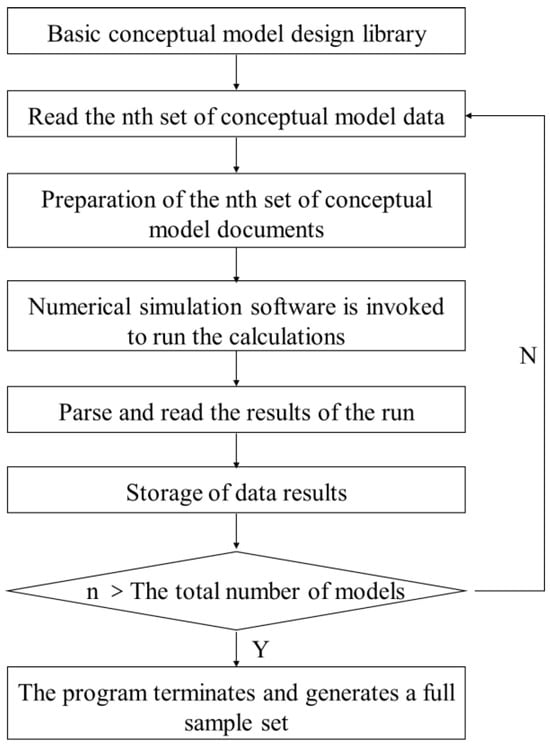
Figure 4. Flowchart of the automated program for numerical simulation scenario generation.

(1) Read Conceptual Model: The program sequentially reads the basic parameters for each conceptual model from the base model design library. These parameters are divided into three parts: first, the fundamental model parameters as listed in Table 3, which include data for modifying permeability, porosity, and grid block size; second, the sidetracking parameters such as timing and well location as specified in Table 4; and third, the input file for the initial conceptual model.

(2) Write Numerical Simulation Input Files: Using relevant Python (version 3.8) libraries, the parameters from the first two parts are batch-written into the initial conceptual model input file according to the established orthogonal experimental design. This process automatically generates the 15,000 corresponding conceptual model scenarios.

(3) Invoke Numerical Simulator: The program calls the external numerical simulation software via Python to run and perform the simulation calculations.

(4) Parse and Read Simulation Results: After the numerical simulator completes a run, a corresponding output data file is generated. The program parses this file to extract parameters required for this study, such as remaining recoverable reserves and oil saturation.

(5) Store Data: The results extracted after each conceptual model simulation are stored.

(6) Conditional Check: The program checks if the number of processed conceptual models is greater than the total number of scenarios in the base model library. If the condition is not met, the process returns to Step 1 to read the parameters for the next model. If the condition is met, the program integrates the output parameters obtained from the simulator with the relevant input parameters from the conceptual model scenarios to form the final conceptual data sample set.

3.2.2. Construction of the Sample Set

Based on the established indicator system and the modeling procedure described above, the origin of the data and the techniques used to gather it for each indicator were specified. Two main gathering techniques are used.

(1) Direct Acquisition: This refers to data that is directly generated by the numerical simulator after running a conceptual model.

(2) Indirect Acquisition: This refers to data that is obtained through processing or converting the directly acquired data.

Based on this analysis, the gathering technique for each indicator in the system was finalized and is summarized in the table below.

According to the aforementioned calculation methods and the results from the numerical simulations, a final sample set comprising 12,000 data groups was collected and compiled. The reduction from the initial number is due to issues such as simulation run failures with some of the conceptual models. A portion of the final dataset is shown in Table 6.

Table 6. Partial sample dataset for machine learning model training.

X-Coordinate	Y-Coordinate	Permeability	Porosity	Effective Thickness (m)	Oil Saturation	Sidetracking Timing	Production Enhancement Rate
30	22	4878.535	0.449	0.499	0.383	70%	1.008
30	22	527.938	0.495	0.580	0.393	70%	1.005
30	22	2861.127	0.212	2.246	0.393	70%	0.995
30	22	5013.696	0.318	0.920	0.393	70%	0.994
30	22	1959.271	0.258	2.125	0.393	70%	0.994
41	26	1548.168	0.407	2.607	0.403	80%	1.003
41	26	5875.064	0.235	1.851	0.404	80%	0.992
41	26	1855.819	0.442	2.721	0.404	80%	0.992
41	26	5426.663	0.477	1.050	0.404	80%	0.992
41	26	580.033	0.272	2.058	0.404	80%	0.994
31	26	2854.517	0.336	2.284	0.469	90%	1.009
31	26	648.454	0.246	0.805	0.469	90%	1.000
31	26	4309.281	0.339	2.192	0.469	90%	0.996
31	26	3549.780	0.406	2.096	0.470	90%	0.995
31	26	2133.431	0.309	0.785	0.470	90%	0.996

4. Data-Driven Prediction Algorithms for Sidetracking Development Performance

The study of sidetrack well placement optimization aims to identify the optimal design plan for sidetracking development. The optimization process requires an accurate prediction of the development performance under various sidetracking scenarios to obtain key performance indicators, such as the production enhancement rate. This necessitates the construction of an efficient and accurate predictive model for sidetracking performance.

Currently, there are few methods specifically for production or performance forecasting related to sidetrack wells. The limited existing research primarily involves analytical methods based on reservoir engineering theory. Although such analytical approaches are computationally straightforward, their practical application is somewhat limited. Machine learning techniques have gained significant traction in recent research for forecasting the performance of conventional oil wells. Given the analogous nature of sidetrack and conventional wells, this chapter therefore assesses and selects from established machine learning prediction methods. Based on the previously prepared sidetrack well design data sample set, this study constructs multiple machine learning prediction algorithms and evaluates their effectiveness. Ultimately, an intelligent prediction model suitable for forecasting sidetracking development performance is selected and established.

4.1. Initial Selection of Machine Learning Algorithms

In traditional reservoir performance prediction, regression models are a relatively common forecasting method [27]. A regression prediction model is a statistical approach that primarily investigates the causal relationship between independent and dependent variables. The fundamental principle of a regression model is to establish a mathematical model describing this relationship by analyzing existing data. For this study, four common regression models were selected: Linear Regression, Polynomial Regression, Random Forest, and a Backpropagation (BP) Neural Network.

4.1.1. Construction and Evaluation of Regression Prediction Models

For this study, the input values for the prediction models included 19 geological and development parameters, specifically: Oil Saturation at the Well Location, Remaining Recoverable Reserves, Field-wide Average Permeability, Field-wide Average Porosity, Average Water Cut, Field-wide Total Thickness, Coefficient of Variation for Permeability, Coefficient of Variation for Porosity, Coefficient of Variation for Effective Thickness, Permeability Grade Difference, Porosity Grade Difference, Effective Thickness Grade Difference, Permeability, Porosity, Effective Thickness, Recovery Factor, Well Drainage Area, Oil Saturation at Target, and Initial Water Cut; and 4 sidetracking design parameters, specifically: Injector-Producer Well Spacing, Distance between the new sidetrack and the original wellbore, Sidetrack Target Location, and Sidetracking Timing. It should be noted that the X and Y coordinates of the sidetrack well are not used as input indicators for the prediction models because the “Injector-Producer Well Spacing” and the “Distance between the new sidetrack and the original wellbore” have a direct geometric relationship with the X and Y coordinates. The output of the prediction model is the Production Enhancement Rate. The study utilizes a total of 12,000 data samples, of which 80% is allocated to the training set and the remaining 20% is used as the validation set.

(1) Linear Regression

Linear Regression is a method used to establish a linear relationship between independent and dependent variables [28]. Specifically, the loss curves for the model’s training and test sets and the cross-validation prediction plot as shown in Figure 5, Figure 6 and Figure 7.

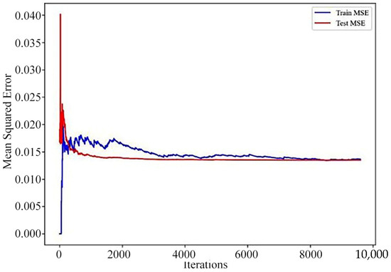
Figure 5. Multiple linear regression model loss curves.

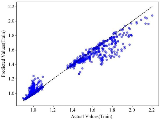
Figure 6. Multiple linear regression model cross-validation prediction (training set).

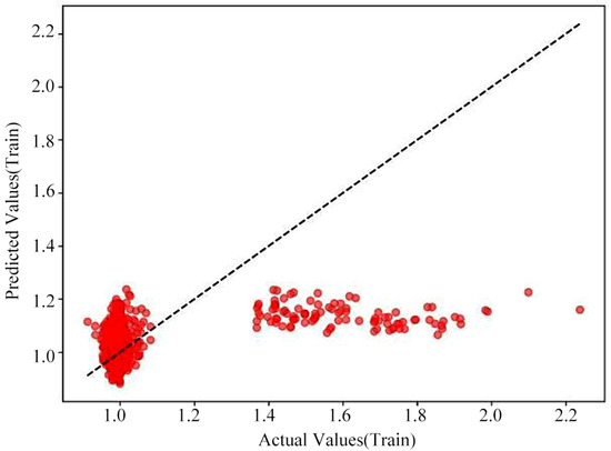
Figure 7. Multiple linear regression model cross-validation prediction (test set).

(2) Polynomial Regression

Polynomial Regression is distinct from the Linear Regression model, as it fits the input–output relationship of the data using a curve, rather than being restricted to a straight line. It is suitable for fitting nonlinear data, approximating the true relationship within the data by increasing the degree of the polynomial [29]. Specifically, the loss curves for the model’s training and test sets and the cross-validation prediction plot as shown in Figure 8, Figure 9 and Figure 10.

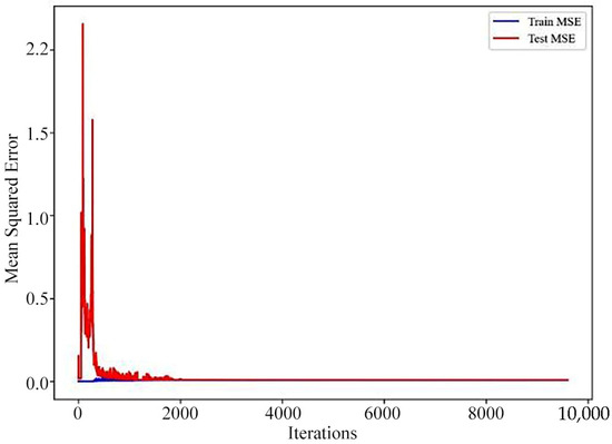
Figure 8. Polynomial regression model loss curve.

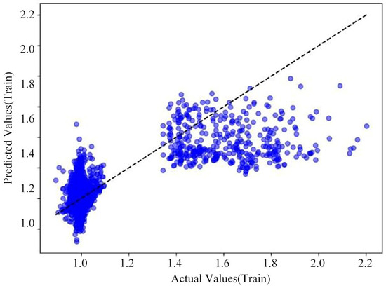
Figure 9. Polynomial regression model cross-validation prediction (training set).

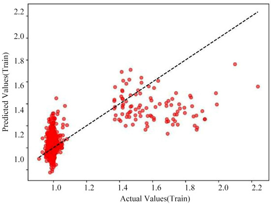
Figure 10. Polynomial regression model cross-validation prediction (test set).

(3) Random Forest

Random Forest is an ensemble learning method that makes its final decision by aggregating the predictions of multiple decision trees. This method helps to reduce overfitting and performs excellently when handling large datasets [30]. The basic flowchart for constructing a Random Forest is shown below. Specifically, the loss curves for the model’s training and test sets and the cross-validation prediction plot as shown in Figure 11, Figure 12 and Figure 13.

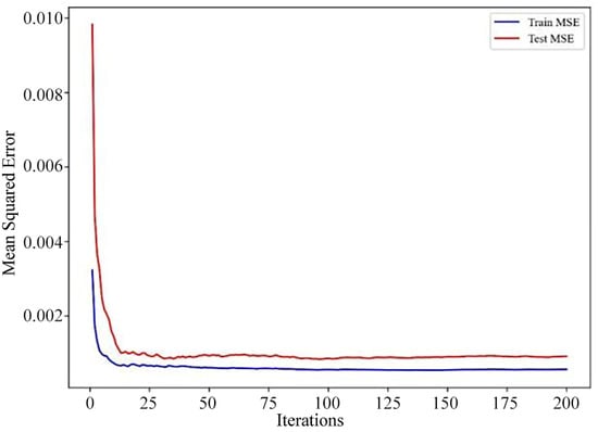
Figure 11. Random Forest model loss curves.

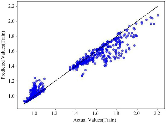
Figure 12. Cross-validation prediction for the Random Forest model (training set).

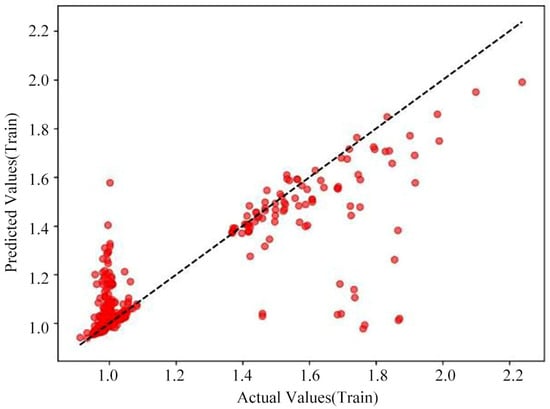
Figure 13. Cross-validation prediction for the random forest Model (test set).

The MSE for the Random Forest model’s training set is 0.0008, and the MSE for the test set is 0.0011; the R² for the training set is 0.9524, and the R² for the test set is 0.7842. Based on these training evaluation metrics for the Random Forest model, its training performance is excellent. As illustrated by the Random Forest model’s loss curve in Figure 11, both the training and test sets demonstrate a strong goodness of fit. While Figure 13 indicates some discrepancies between the predicted and true values for the test set, the Random Forest model’s overall training performance is nonetheless considered very good.

(4) BP Neural Network

The BP Neural Network represents a common and widely adopted class of artificial neural network [31]. When constructing the BP Neural Network, the training sample set selection was consistent with the previously mentioned models. The sample data is preprocessed using normalization, the calculation formulas are shown in Formula (1).

$$X_n={\displaystyle \frac{X-X_{\min }}{X_{\max }-X_{\min }}}$$

(1)

In this formula, $X_n$ represents the normalized data, $X$ is the original data to be normalized, $X_{\min }$ denotes the row vector containing the minimum value of each column, and $X_{\max }$ denotes the row vector containing the maximum value of each column.

This dataset was partitioned, with 80% allocated to the training set and 20% reserved for the test set. A foundational BP Neural Network architecture consists of an input layer, hidden layers, and an output layer. The input layer contains 23 nodes, corresponding to the 23 input features. There are 23 neurons in the first hidden layer, and the number of neurons in the output layer is consistent with the number of output indicators, which is 1. The activation function for this BP Neural Network is ReLU. The specific architectural parameters of this neural network as shown in Table 7.

Table 7. Architecture of the BP Neural Network.

Indicator	Parameters
Input Layer	23
Hidden Layer	23
Output Layer	1
Epochs	400
Dropout	0.2
Optimizer	Adam()
Activation Function	ReLU

The loss curves for the training and test sets of the BP Neural Network prediction model and the cross-validation prediction plot as shown in Figure 14, Figure 15 and Figure 16.

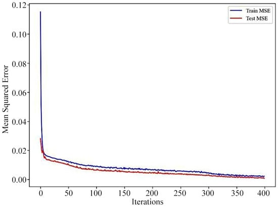
Figure 14. BP Neural Network model loss curve.

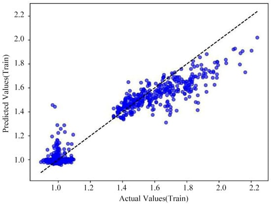
Figure 15. Cross-validation prediction for the BP Neural Network model (training set).

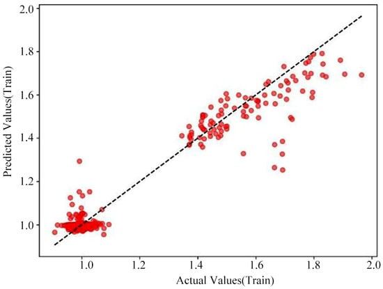
Figure 16. Cross-validation prediction for the BP Neural Network model (test set).

The MSE for the BP Neural Network model’s training set is 0.0034, and the MSE for the test set is 0.0042; the RMSE for the training set is 0.0583, and the RMSE for test set is 0.0648; the R² for the training set is 0.7935, and the R² for the test set is 0.7585. Based on the results of these training evaluation metrics for the BP Neural Network model, the model’s training fit is relatively good; however, according to the predicted versus true values for the model’s training and test sets shown in Figure 15 and Figure 16, a considerable error still exists. It should be noted that this architecture represents a relatively basic configuration. It is included here primarily as a baseline model for comparison. While more complex deep learning architectures could be explored in future work, the Random Forest model already demonstrated superior performance to this baseline model, as detailed in the comprehensive comparison.

4.1.2. Comprehensive Comparison of Regression Prediction Models

Four models were compared using MSE, RMSE, and R² as metrics. The results are summarized in Table 8.

Table 8. Prediction model comprehensive evaluation.

Model Name	Train Set MSE	Test Set MSE	Train Set RMSE	Test Set RMSE	Train Set R2	Test Set R2
Linear Regression	0.0136	0.0134	0.1166	0.1158	0.1839	0.1651
Polynomial Regression	0.0076	0.0083	0.0872	0.0911	0.5456	0.4850
Random Forest	0.0008	0.0011	0.0283	0.0332	0.9524	0.7842
BP Neural Network	0.0034	0.0042	0.0583	0.0648	0.7935	0.7585

According to the training performance evaluation results for the various prediction models in Table 8, it is evident that the models based on Random Forest and BP Neural Networks demonstrate superior training performance. However, in terms of both the MSE RMSE and R² metrics for both training and testing data, the Random Forest predictor achieves better results than the BP Neural Network model. This suggests that the Random Forest model provides a better goodness of fit compared to the BP Neural Network. In summary, the Random Forest model was chosen as the predictive tool for the sidetracking development performance indicators.

4.2. Random Forest Model Hyperparameter Optimization

Based on the preceding research, which involved the analysis and evaluation of multiple prediction models, the Random Forest model was ultimately selected as the predictive model for sidetracking development performance. For machine learning models, hyperparameters are parameters of extreme importance. To further enhance the predictive performance of the Random Forest model, this paper will optimize two of its hyperparameters: the “number of decision trees” and the “maximum depth of the trees”.

This study uses the Grid Search method for Random Forest hyperparameter optimization [32]. Grid Search is a technique for tuning hyperparameters; it operates by exhaustively searching through a specified parameter space to identify the combination that yields the best model performance. This helps to avoid the tedious work of manually tuning hyperparameters.

In the initial model tests mentioned earlier, the Random Forest configuration used 200 decision trees and a maximum depth of 15. For the subsequent hyperparameter optimization of this Random Forest model via the Grid Search method, the designated optimization parameters as shown in Table 9.

Table 9. Hyperparameter indicator range setting.

Indicator Name	Indicator Range
Number of Decision Trees	[100, 200, 300, 400]
Maximum Tree Depth	[5, 10, 15, 20]

For the hyperparameter optimization training of the Random Forest model, the data sample set was selected in the same manner as for the previously described prediction models. The dataset was likewise partitioned into an 80% training set and a 20% validation set. After screening through different hyperparameter combinations and model training sessions, it was found that the Random Forest model’s optimal training performance occurred with 300 decision trees and a maximum tree depth of 20. The performance graphs for this optimized model as shown in Figure 17, Figure 18 and Figure 19.

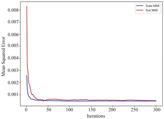
Figure 17. Loss curve of the optimized Random Forest model.

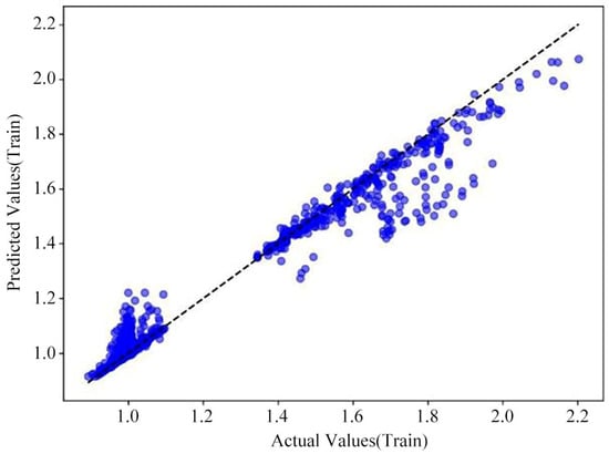
Figure 18. Optimized Random Forest model cross-validation prediction (training set).

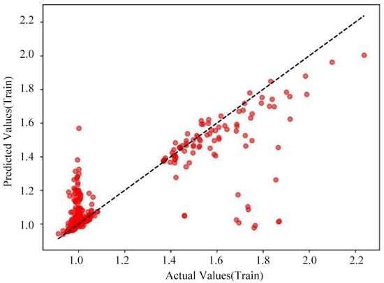
Figure 19. Optimized Random Forest model cross-validation prediction (test set).

The hyperparameter-optimized Random Forest model achieved an MSE of 0.0004 on the training set and 0.0008 on the test set, with corresponding R² values of 0.9722 and 0.8059, respectively. A comparison table of the training evaluation metrics against the pre-optimization Random Forest model is shown in Table 10.

Table 10. Comparison of Random Forest model training evaluation indicators before and after optimization.

Model Name	Train Set MSE	Test Set MSE	Train Set RMSE	Test Set RMSE	Train Set R2	Test Set R2
Random Forest Model	0.0008	0.0011	0.0283	0.0332	0.9524	0.7842
Random Forest Model after Hyperparameter Optimization	0.0004	0.0008	0.02	0.0283	0.9722	0.8059

When comparing the training results of the Random Forest model before and after optimization, the model post-hyperparameter tuning exhibits a notable improvement in performance across all evaluation metrics relative to the original model. Based on the model’s loss curve as shown in Figure 17, the goodness of fit for both the training and test sets is also excellent. As shown in Figure 18, the error between the true and predicted values for the model’s training set is small. While for the test set, shown in Figure 19, some error exists between certain predicted and true values, the optimized Random Forest model, on the whole, meets the required standards for predicting sidetracking development performance.

5. Mathematical Model Development and Solution for Sidetrack Well Placement Optimization

For developing and solving the mathematical model for sidetrack well placement optimization, the core of its objective function is based on the previously established intelligent prediction model for sidetracking development performance. Secondly, the selection of the optimization algorithm is also of critical importance. For the sidetrack well placement optimization problem, as well as for other conventional well pattern optimization problems, two main aspects are generally considered: first, how to select a suitable and efficient optimization algorithm for the specific optimization problem, and second, how to construct and debug the algorithm to handle different constraints. This chapter will provide a detailed discussion of the aforementioned issues.

5.1. Mathematical Model for Sidetrack Well Placement Optimization

Well placement optimization is a common class of problems in the oil and gas industry, which seeks to optimize well locations to reduce extraction costs, increase production, minimize environmental impact, or meet specific geological and engineering requirements. In this work, a mathematical model is constructed for sidetrack well placement optimization based on optimization algorithms to further identify the optimal sidetrack location. The optimization goal of this study is to maximize the Production Enhancement Rate, and the optimal solution refers to the sidetrack well placement configuration that achieves this objective under all defined constraints.

The establishment of a mathematical optimization model generally requires consideration of the following four aspects: namely, the performance indicator, decision variables, the objective function, and any constraints. Grounded in these four elements, the mathematical model for sidetrack well placement optimization in this paper is elaborated as follows:

(1) Performance Indicator

Performance indicators for evaluating sidetracking development performance typically include metrics such as stable production period and cumulative oil production. In the second chapter of this paper, the “Production Enhancement Rate” was defined as the performance indicator for evaluating sidetracking development performance. It reflects the change in the well’s production rate before and after sidetracking.

(2) Decision Variable

The decision variables to be optimized are identified; these are the input parameters that influence the objective function and are typically represented as a vector, $A={(a_1,a_{2,\dots },a_n)}^T$, where different combinations of these parameters form different well placement design scenarios.

For the well placement optimization problem, the primary decision variables are the specific locations of each wellhead. Specifically, in the well pattern considered in this study, the locations of the injection wells are kept constant. Therefore, the optimization of the well location only includes the planar x-coordinate (X) and y-coordinate (Y) of the production well’s sidetrack target, the timing of the sidetracking, and the determination of the optimized sidetrack layer. Once the optimized sidetrack location for the production well is determined, the specific optimized values for the injector–producer spacing, the distance from the target to the original wellbore, and the target’s position can also be determined.

(3) Objective Function

The objective function represents the quality of a design scenario and is often denoted by P(X). The objective of sidetrack well placement optimization is to determine the location for the production well’s sidetrack that enables more efficient production. In terms of the performance indicator, this translates to maximizing the “Production Enhancement Rate,” thereby ensuring the greatest possible improvement in development performance after sidetracking. In the third chapter of this paper, the training performance of six prediction models was compared. Through a comparison of the final evaluation metrics, it was determined that the Random Forest model exhibited the best performance in predicting sidetracking development outcomes, and this model was subsequently hyperparameter-tuned. Therefore, the trained Random Forest model was established as the objective function in the mathematical model for well placement optimization. The fully trained Random Forest model is saved so that it can be called within the code of the mathematical optimization model. To facilitate solving with optimization algorithms, the problem of maximizing the “Production Enhancement Rate” is converted into a standard minimization problem. Specifically, we define the objective function as the negative of the predicted Production Enhancement Rate. Therefore, the mathematical expression for the optimization model is $\min P(a)=P(a_1,a_2,\dots ,a_n)$, where $a$ = ($a_1,a_2,\dots ,a_n$) is the vector of decision variables.

(4) Constraints

For the construction of an optimization algorithm, the constraints are primarily the limiting conditions imposed on the decision variables. They are typically expressed as $R_i(a)\le 0$, where $i=1,2,\dots ,k$ and where k represents the total number of constraints.

For the sidetrack well placement optimization problem in this study, the specific constraints involved include the upper and lower bound constraints for the sidetrack well location ($X$,$Y$), the constraint on the sidetracking timing ($T$), the constraint on the target location ($D_z$), and the minimum well spacing constraint ($d^{\min }$), the calculation formulas are shown in Formulas (2)–(6).

(a) Upper and lower bound constraints for the sidetrack well location:

$$x^{\min }<X<x^{\max }$$

(2)

$$y^{\min }<Y<y^{\max }$$

(3)

(b) Sidetracking timing constraint:

$$70\%<T<95\%$$

(4)

(c) Target location constraint ($D_z$):

$$0<D_z<1$$

(5)

(d) Minimum well spacing constraint, which ensures the distance between two wells is not less than a given minimum well spacing:

$$\sqrt{{(x_i-x_j)}^2+{(y_i-y_j)}^2}\le d^{\min }$$

(6)

5.2. Preliminary Selection of Optimization Algorithms

Through a literature review and research, it is known that a wide variety of optimization algorithms currently exist. First, a preliminary selection of various optimization algorithms is required to identify those suitable as candidates for the well placement optimization problem. Drawing upon established engineering experience, an initial selection was made, which included the Multilevel Coordinate Search (MCS) algorithm, the Differential Evolution (DE) algorithm, and the Covariance Matrix Adaptation Evolution Strategy (CMA-ES) were preliminarily selected. These three algorithms each have distinct characteristics: the DE optimization algorithm has strong global optimization capabilities; MCS and CMA-ES also possess global search capabilities, but their performance may vary depending on parameter settings and algorithmic design; CMA-ES is suitable for a broader range of problem types, including non-smooth and high-dimensional problems.

Choosing between these algorithms is contingent upon the problem’s specific characteristics and dimensionality, along with the necessary trade-off between global and local search capabilities. Concurrently, the algorithm best suited for solving the sidetrack well placement optimization problem will be chosen based on the evaluation criterion of superior performance in this specific application.

(1) Multilevel Coordinate Search Algorithm

The Multilevel Coordinate Search (MCS) algorithm is a global optimization method developed to locate the optimal solution for intricate problems. It enhances the efficiency of solving global optimization problems by decomposing the search problem into multiple levels or stages and coordinating the search process across these levels, which makes MCS a powerful tool for handling complex optimization problems [33].

Based on the content of this study, the relevant parameters for this algorithm were set as shown in Table 11.

Table 11. MCS algorithm parameter setting.

Parameter	Value	Description
Number of Levels	3	The stages of decomposition for the complex search space.
Local search sample size	15	The number of samples used for local refinement around the best point found at each stage.
Max Iterations	1000	The upper limit on the number of generations before the algorithm terminates.
Population Size	20	The number of candidate solutions maintained and evaluated in each iteration.
Convergence Threshold	10−6	A stopping criterion; the algorithm terminates if the improvement in the best solution’s fitness falls below this value.

(2) Differential Evolution (DE) Optimization Algorithm

The Differential Evolution (DE) algorithm is a global search strategy that utilizes a population-based search method. It progressively modifies the parameters of individuals within the search space, updating these parameters through a differential operation, with the expectation of gradually optimizing the search results. Due to its small number of parameters and relatively simple implementation, DE has achieved widespread success in practical applications [34]. Based on the content of this study, the relevant parameters for this algorithm were set as shown in Table 12.

Table 12. DE algorithm parameter setting.

Parameter	Value	Description
Strategy	randtobest1bin	The specific mutation and crossover method used to generate new candidate solutions.
Population Size	15	The number of candidate solutions maintained and evaluated in each iteration.
Max Iterations	1000	The upper limit on the number of generations before the algorithm terminates.
Convergence Threshold	10−6	A stopping criterion; the algorithm terminates if the improvement in the best solution’s fitness falls below this value.

(3) Covariance Matrix Adaptation Evolution Strategy (CMA-ES)

The Covariance Matrix Adaptation Evolution Strategy (CMA-ES) is an evolutionary algorithm used for solving continuous parameter optimization problems. By maintaining and adjusting an adaptive covariance matrix, CMA-ES can efficiently adapt to the characteristics of different problems, thereby achieving a faster optimization process [35]. Regarding the parameter settings for the CMA-ES algorithm, according to the algorithm’s designers, the parameters have already been taken into account during the algorithm’s design process. As shown in Table 13, the CMA-ES algorithm has several built-in parameter settings. The parameters are primarily set automatically based on the problem’s dimensionality. Consequently, this algorithm does not require extensive manual parameter tuning during use; one only needs to provide an initial solution and the corresponding variance for that initial solution.

Table 13. CMA-ES algorithm parameter setting.

Parameter	Value	Description
Population Size ($\lambda$)	$4+⌊3\ln (n)⌋$	The number of new candidate solutions, or offspring, generated in each generation. Its size is typically set dynamically based on the problem dimension, $n$.
Parent Population Size ($\mu$)	$⌊\lambda /2⌋$	The number of best-performing individuals selected from the $\lambda$ offspring. These parents are used to update the mean, step-size, and covariance matrix for the next generation.
Learning Rate for Rank-One Update ($c_c$)	${\displaystyle \frac{4}{(n+4)}}$	The learning rate for updating the covariance matrix using the “evolution path”. It helps the algorithm utilize information from the history of movements to adapt to correlations between variables.
Learning Rate for Step-Size Control ($c_{\sigma }$)	${\displaystyle \frac{{\mu }_{eff}+2}{n+{\mu }_{eff}+3}}$	The learning rate for adapting the global step-size (search radius). It allows the algorithm to dynamically increase or decrease the search range based on the progress of the search.

For consistency and to ensure quantitative comparability, the CMA-ES algorithm was executed under the same convergence threshold (10⁻⁶) and maximum iteration limit (1000) as MCS and DE. In the CMA-ES algorithm, $n$ represents the dimension of the problem (i.e., the number of decision variables), and ${\mu }_{eff}$ is the “effective number of parents” derived from weighted recombination. These parameters are typically calculated internally by the algorithm using recommended formulas and do not require manual setting.

5.3. Comparison of Algorithm Performance in Well Placement Optimization

The optimization algorithms are used to directly solve the sidetrack well placement optimization problem. The basic solution procedure is as follows: First, an initial value is generated based on the defined constraints, for example, by selecting the median value of the constraints. Next, this initial value, combined with the original reservoir geological and development parameters, is fed into the trained sidetracking development performance prediction model to forecast the corresponding production enhancement rate. Then, a judgment is made based on the resulting production enhancement rate to determine if the termination condition is met. If it is not met, the optimization algorithm will automatically update and generate a new generation of decision variable combinations until the termination condition is satisfied. Finally, the optimal combination of decision variables is output, forming the best sidetracking development design plan. The specific solution flowchart is shown in Figure 20.

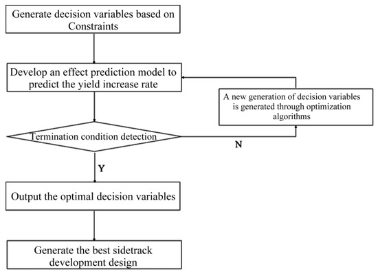
Figure 20. Optimization algorithm solution flowchart.

5.3.1. Test Model Introduction

For the testing of the sidetrack well placement algorithm, a waterflood reservoir model was selected. This model includes two phases, oil and water, and contains a total of five wells: four injection wells and one production well. The reservoir model has a permeability of 4878.535 mD, a porosity of 0.449, an average water cut of 95%, and a formation pressure of 16.899 MPa. As shown in Figure 21 and Figure 22 the permeability and initial well location map and the depth map in the Z-direction for this model.

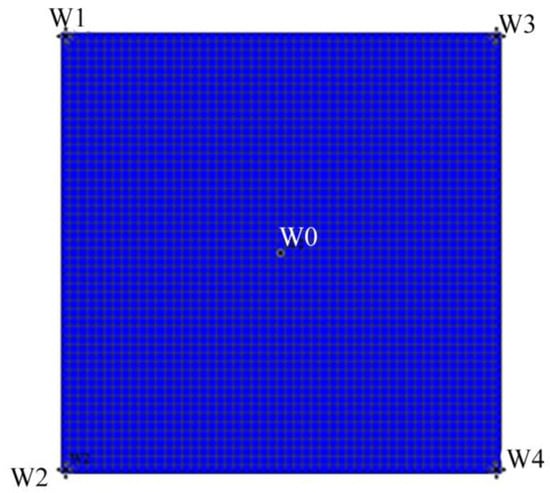
Figure 21. Permeability map and initial well location map of the optimization algorithm test model.

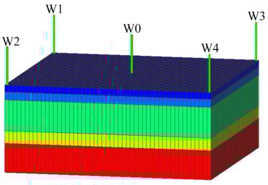
Figure 22. Three-dimensional depth structure of the optimization algorithm test model.

Well placement optimization is performed on the one production well in this model. There are a total of four optimization variables: the sidetrack target X-coordinate, the sidetrack target Y-coordinate, the target location, and the sidetracking timing. For the upper and lower bound constraints on the well position ($X$,$Y$), the ranges are 26 < $X$ < 51 and 1 < $Y$ < 26. The upper and lower bound constraint for the target location ($D_z$) is 0 < $D_z$ < 1, and the upper and lower bound constraint for the sidetracking timing ($T$) is 0.7 < $T$ < 0.95. The MCS, DE, and CMA-ES algorithms are used to solve this problem.

5.3.2. Algorithm Performance Comparison

The performance of the MCS, DE, and CMA-ES algorithms in solving the well placement optimization problem are shown in Figure 23, Figure 24 and Figure 25. Within these figures, the x-axis denotes the count of objective function evaluations, while the y-axis indicates the optimal production enhancement rate.

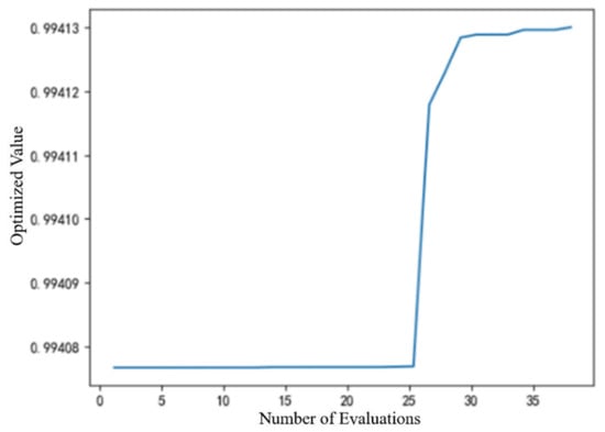
Figure 23. Iteration process for the MCS optimization algorithm.

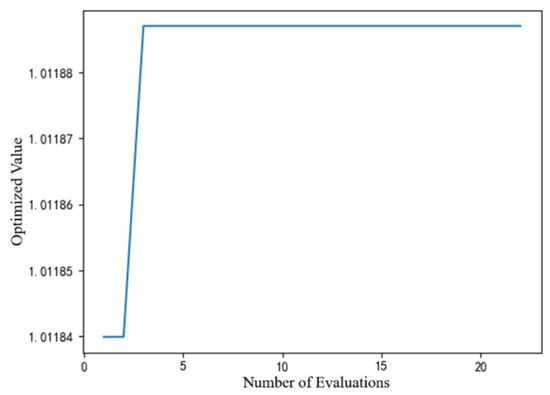
Figure 24. DE optimization algorithm’s iterative process.

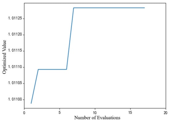
Figure 25. Iterative optimization process for the CMA-ES algorithm.

As shown in Figure 23, the MCS algorithm requires almost 40 function evaluations to begin converging. In contrast to the other two algorithms (Figure 24 and Figure 25), the MCS method fails to achieve the global optimum, showing a persistent small gap. In contrast, the DE algorithm shown in Figure 24 finds the optimal solution on the third evaluation, while the CMA-ES algorithm shown in Figure 25 reaches the optimum value on the seventh evaluation. From this perspective, it is clear that the DE and CMA-ES optimization algorithms outperform the MCS optimization algorithm.

Both DE and CMA-ES are stochastic algorithms, meaning their results can vary between runs. To quantitatively assess the repeatability and robustness of these two algorithms, each was executed 10 times under identical initial conditions. The results of this repeatability analysis are shown in Figure 26 and Figure 27.

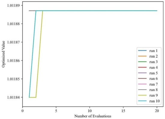
Figure 26. Stochastic analysis of DE optimization algorithm.

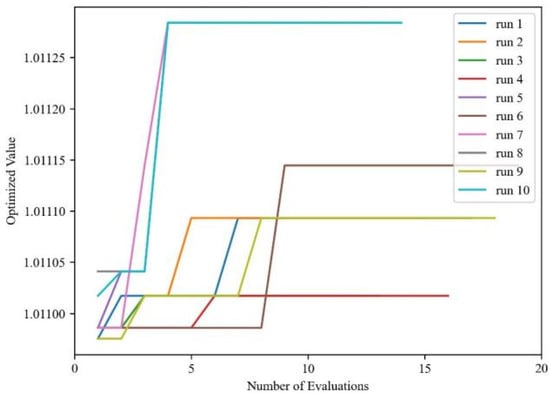
Figure 27. Stochastic analysis of CMA-ES optimization algorithm.

From the figures, it can be seen that both the DE and CMA-ES optimization algorithms do indeed exhibit stochasticity. The DE algorithm demonstrates relative stability, converging at the latest after the fourth iteration. In contrast, the results of the CMA-ES algorithm after 10 consecutive optimization runs show extreme instability, and it converges to the optimal solution, at the latest, only after the 11th iteration. From this perspective, the CMA-ES algorithm is not only highly stochastic but also struggles to obtain the optimal solution after multiple calculations, and it requires more iterations to achieve the optimal result compared to the DE algorithm.

The actual computational results of the MCS, DE, and CMA-ES algorithms were statistically compiled. For the DE and CMA-ES algorithms, the result selected was the one that occurred with the highest frequency among the ten runs for each respective algorithm. The specific operational data for each optimization algorithm is shown in Table 14.

Table 14. Performance and result comparison of the three optimization algorithms.

Algorithm Name	Optimal Production Enhancement Rate	Optimal Result				Run Time (s)
		Target X-Coordinate	Target Y-Coordinate	Target Location	Sidetracking Timing
MCS	0.9942	32	25	3/5	0.89	40.7758
DE	1.0119	32	10	2/5	0.85	65.3507
CMA-ES	1.0113	32	12	2/5	0.83	31.5789

Combining the preceding analysis with the results in the table, it is clear that the MCS and CMA-ES algorithms require less computation time, but the convergence performance of the MCS algorithm is relatively mediocre. The solution results of the DE algorithm are quite close to those of the CMA-ES algorithm. Although the CMA-ES algorithm has an advantage in terms of run time, the DE algorithm is superior in terms of the number of iterations required to find the optimal solution. Furthermore, due to the excessive stochasticity of the CMA-ES algorithm, it is difficult to obtain the optimal solution even after multiple repeated calculations. Therefore, in summary, in the performance comparison for the sidetrack well placement optimization mathematical model, the DE algorithm exhibits the best overall performance.

6. Application Case Study and Performance Analysis

6.1. Field Validation of Algorithm Performance for Well Placement Optimization

The application case block is situated in the southern part of the field, possessing an overall structural morphology that is high in the southeast and low in the northwest. The structure is raised near the boundary fault and dips at its periphery. The target well area is situated on the margin of a sand body in the homogeneous zone of the block, with a simple and gentle overall structure. The reservoir is shallowly buried with loose cementation, and its rock surface is hydrophilic. Based on core data from the area, the target block’s average porosity is 33.5%, with an effective permeability is 937 × 10⁻³ µm², the original oil saturation is 65%, and the clay content is 6.5%. The target well area has a permeability of 963 × 10⁻³ µm² and an average effective porosity of 32.4%.

In the target well area, the average surface crude oil viscosity is 973 mPa·s, and the CaCl₂ type formation water has a total salinity of 6518 mg/L. The average surface degassed crude oil density is 0.979 g/cm³, the average surface crude oil viscosity is 1650 mPa·s, and the formation water is predominantly of the NaHCO₃ type. For the produced water, the current total salinity is 9856 mg/L.

Both the temperature and pressure systems in this application case block are normal. Block-wide, the original formation pressure ranges from 13.4 to 14.6 MPa, with an original saturation pressure of 9.9 MPa, an original gas–oil ratio of 26.3 m³/t, a formation pressure coefficient of 1.04, and a geothermal gradient of 3.4 °C/100 m. The original formation temperature in the target well area is 65 °C, the original formation pressure is 13.9 MPa, and the saturation pressure is 8.7 MPa. The well area designated for sidetracking has a drainage area of 0.056 km², an average effective thickness of 5.6 m, geological reserves of 6.3 × 10⁴ t, remaining controlled reserves of 4.6 × 10⁴ t, and remaining recoverable reserves of 0.9 × 10⁴ t, providing a substantial material basis for a sidetracking operation.

Currently, a suite of advanced equipment based on intelligent systems and cloud computing has been deployed in the application case area to enable the automatic collection of core oil and gas production parameters. This initiative provides strong support for evaluating the practical field application and performance of this project’s outcomes.

6.2. Sidetrack Well Placement Optimization and Performance Analysis for the Target Block

Since the complete application case block model includes multiple production and injection wells, a smaller section was extracted from the complete block model to avoid the influence of these other wells, while still satisfying the injector–producer relationship for the target sidetrack well. This extracted section is shown in Figure 28 and Figure 29. Red represents oil, blue represents water, and the other colors indicate lower oil saturation.

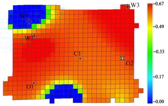
Figure 28. Well location and oil saturation distribution map for the application case block.

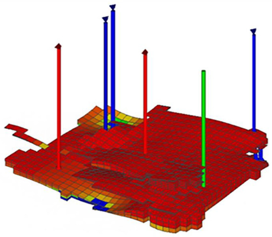
Figure 29. Three-dimensional geological model of the application case block.

Based on Figure 28 and Figure 29, in the application case block model, C1 is the target sidetrack well, with a daily fluid production of 16.4 tons, daily oil production of 2.5 tons, and a water cut of 85.0%. W1, W2, and W3 are injection wells. O1 is a nearby production well with a daily fluid production of 14.5 tons, daily oil production of 1.4 tons, and a water cut of 90.4%. O2 is a shut-in production well. The degree of water flooding in the well area is low, and there is an abundance of remaining oil.

In the original plan, the target sidetrack well had perforations in five layers and was sidetracked in the fourth layer. To meet the data requirements of the sidetrack well placement optimization algorithm developed in this study, the five layers of this model were vertically refined with greater detail. Each layer was subdivided into five sublayers of equal grid thickness, resulting in a 25-layer reservoir model. Following this, the necessary data was collected and organized.

The formulation of the mathematical model for sidetrack well placement optimization requires the integration of a sidetracking development performance prediction model with an intelligent optimization algorithm. The sidetracking performance prediction model is established using original geological and development parameters along with new sidetrack well indicators as inputs, and sidetracking performance indicators as the output; it is continuously tuned to achieve optimal performance. In conjunction with an optimization algorithm, the post-sidetracking performance indicators are synthesized into a single performance evaluation metric. With the four new sidetrack well indicators as input, an iterative calculation is performed to find the four new sidetrack well indicators that maximize this evaluation metric. It is important to note that among the new sidetrack well indicators, the injector-producer spacing and the distance from the target to the original wellbore have a direct conversion relationship with the X and Y coordinates of the sidetrack well. Therefore, the actual decision variables obtained through the sidetrack well placement optimization algorithm are the X and Y coordinates of the sidetrack target, the target location, and the sidetracking timing.

Based on the preceding research, the Random Forest model was selected as the sidetracking development performance prediction model, and the DE algorithm was chosen as the intelligent optimization algorithm. By integrating the aforementioned intelligent prediction model and optimization algorithm, the original geological and development parameters of the “target block model” are held constant. The four new sidetrack well indicators are used as inputs, and the production enhancement rate is selected as the comprehensive evaluation metric for the DE optimization algorithm. To avoid a situation where a single run yields an exceptionally good or exceptionally poor result due to the stochastic nature of the DE algorithm, the algorithm was run ten times repeatedly, and the optimal value combination that occurred with the highest frequency among the results was selected. To better analyze the accuracy of this optimization plan, both the pre- and post-optimization plans were simulated using numerical simulation software (schlumberger eclipse 2023.1.0) to predict the oil production performance after 15 years of development. The production data from the well before any sidetracking was also included for comparison. The “Pre-Optimization” plan refers to the original sidetracking design proposed by the field engineers, which serves as a baseline for evaluating the optimized plan, while the “Post-Optimization” plan represents the improved design obtained through the proposed data-driven framework.

The specific pre- and post-optimization results are presented in Table 15, while Figure 30 and Figure 31, respectively, illustrate the changes in water cut and cumulative oil production over 15 years for the cases before sidetracking and for the pre- and post-optimization plans.

Table 15. Comparison of pre-optimization and post-optimization solutions.

Indicator Name	Pre-Optimization	Post-Optimization
Sidetrack Target X-Coordinate	13	14
Sidetrack Target Y-Coordinate	12	9
Sidetracking Timing	0.68	0.79
Target Location	Middle of the fourth target layer	Middle of the third target layer
Production Enhancement Rate	0.1927	0.2201

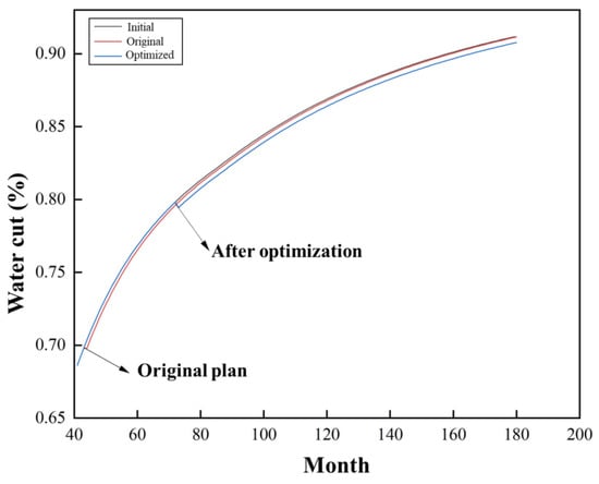
Figure 30. Comparison of water cut schemes.

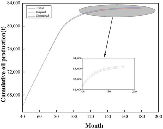
Figure 31. Comparison of cumulative oil production schemes.

As shown in Table 15, the “Post-Optimization” plan, derived from the data-driven framework, achieved a Production Enhancement Rate of 0.2201, which is superior to the original engineer’s “Pre-Optimization” plan rate of 0.1927. To further validate the optimization effect, 15-year numerical simulations were conducted for both plans (Original and Optimized), alongside the “Initial” case (without sidetracking). The results are shown in Figure 30 and Figure 31.

These simulation results provide a clear quantitative before-and-after comparison:

(1) Cumulative Oil Production: As illustrated in Figure 31, the optimized plan resulted in an incremental cumulative oil production of 82.7 tons compared to the original sidetracking plan.

(2) Water Cut: As shown in Figure 30, while both sidetracking plans reduced the water cut at their respective implementation times, the decline in water cut for the optimized plan was more pronounced and remained lower throughout the production period.

This set of clear quantitative results—an improved production enhancement rate from the proxy model, a tangible increase in simulated cumulative oil production, and a more significant water cut reduction—confirms the effectiveness and practical value of the proposed optimization framework.

Based on the pre- and post-optimization plan comparison table as shown in Table 15, it is clear that the production enhancement rate of the optimized plan is superior to that of the previous sidetracking plan. In conjunction with the water cut changes for the three cases as shown in Figure 30, it can be observed that while the water cut decreases at the respective sidetracking times for both the pre- and post-optimization plans, the decline in water cut is more pronounced for the optimized plan overall. Similarly, based on Figure 31, the cumulative oil production of the optimized plan increased by 82.7 tons compared to the original sidetracking plan. In summary, the case study application of the data-driven sidetrack well placement optimization method constructed in this research has demonstrated excellent results.

7. Conclusions

This study proposed and validated an intelligent data-driven decision-making framework for sidetrack well placement optimization, which integrates a machine learning (ML) proxy model with an intelligent optimization algorithm. The main conclusions are as follows:

(1) A standardized indicator system for sidetracking design was established, including 26 parameters in three categories: reservoir geology, sidetracking design, and performance. To overcome the scarcity of real field data, 15,000 conceptual models were generated using Latin Hypercube Sampling and orthogonal design, yielding 12,000 valid samples through an automated simulation workflow as a solid basis for model development.

(2) In solving the performance prediction problem, four regression models were compared, and the Random Forest (RF) model demonstrated the best predictive accuracy. After hyperparameter optimization, the optimized RF model achieved R² values of 0.9722 (training) and 0.8059 (test), proving its reliability as a proxy model for predicting sidetracking outcomes.

(3) For the optimization problem, three algorithms—Multilevel Coordinate Search (MCS), Differential Evolution (DE), and Covariance Matrix Adaptation Evolution Strategy (CMA-ES)—were evaluated. Comparative tests indicated that the DE algorithm achieved the best overall performance in terms of convergence and stability, converging to the optimal solution in fewer iterations and making it a robust choice for this problem.

(4) Finally, the integrated intelligent framework was applied to a real field case. Compared to the original (pre-optimization) plan, the optimized sidetracking plan resulted in a more significant water cut reduction and an incremental cumulative oil production of 82.7 tons, confirming the effectiveness and practical value of the proposed method.

(5) Limitations and Future Work. Despite promising results, the framework has some limitations. The large-scale simulation data generation entails high computational cost, and no formal geological uncertainty analysis was conducted. Moreover, the synthetic training data may cause a “synthetic-to-real” gap. Future work will apply transfer learning or domain adaptation to enhance model generalization with limited field data.

References

- Mansouri, M.; Jafarbeigi, E.; Ahmadi, Y.; Hosseini, S.H. Experimental investigation of the effect of smart water and a novel synthetic nanocomposite on wettability alteration, interfacial tension reduction, and EOR. J. Pet. Explor. Prod. Technol. 2023, 13, 2251–2266. [Google Scholar] [CrossRef]
- Leising, L.J.; Hearn, D.D.; Rike, E.A.; Doremus, D.M.; Paslay, P.R. Sidetracking Technology for Coiled Tubing Drilling. J. Pet. Technol. 1996, 48, 414–421. [Google Scholar] [CrossRef]
- Allan, F.; Shepherd, D.; Abbasov, A. Modelling of Fracture Geometry to Reduce the Risk of Intercepting Drilling Induced Fractures When Designing Sidetrack Trajectories. In Proceedings of the SPE Annual Caspian Technical Conference, Baku, Azerbaijan, 16–18 October 2019; pp. 1–16. [Google Scholar] [CrossRef]
- Lei, Z.; Meng, S.; Peng, Y.; Tao, J.; Liu, Y.; Liu, H. Evaluation of the adaptability of CO2 pre-fracturing to Gulong shale oil reservoirs, Songliao Basin, NE China. Pet. Explor. Dev. 2025, 52, 459–470. [Google Scholar] [CrossRef]
- Magizov, B.; Topalova, T.; Loznyuk, O.; Simon, E.; Orlov, A.; Krupeev, V.; Shakhov, D. Automated Identification of the Optimal Sidetrack Location by Multivariant Analysis and Numerical Modeling. A Real Case Study on a Gas Field. In Proceedings of the SPE Russian Petroleum Technology Conference, Moscow, Russia, 22–24 October 2019. [Google Scholar] [CrossRef]
- Stavychnyi, Y.; Piatkivskyi, S.; Vytiaz, A.; Femiak, V.; Kovbasiuk, M. Specific features and prospects of well recovery by sidetracking based on the example of the Stynava field. Nafta-Gaz 2025, 81, 3–15. [Google Scholar] [CrossRef]
- Jeong, H.; Sun, A.Y.; Lee, J.; Min, B. A learning-based data-driven forecast approach for predicting future reservoir performance. Adv. Water Resour. 2018, 118, 95–109. [Google Scholar] [CrossRef]
- Tadjer, A.; Hong, A.; Bratvold, R.B. Machine learning based decline curve analysis for short-term oil production forecast. Energy Explor. Exploit. 2021, 39, 1747–1769. [Google Scholar] [CrossRef]
- Jiang, H.Y.; Song, Q.; Gao, K.; Song, Q.; Zhao, X. Rule-based expert system to assess caving output ratio in top coal caving. PLoS ONE 2020, 15, e0238138. [Google Scholar] [CrossRef]
- Lu, C.; Jiang, H.; Yang, J. Shale oil production prediction and fracturing optimization based on machine learning. J. Pet. Sci. Eng. 2022, 217, 110900. [Google Scholar] [CrossRef]
- Ojedapo, B.; Ikiensikimama, S.S.; Wachikwu-elechi, V.U. Petroleum Production Forecasting Using Machine Learning Algorithms. In Proceedings of the SPE Nigeria Annual International Conference and Exhibition, Lagos, Nigeria, 1–3 August 2022. [Google Scholar] [CrossRef]
- Makhotin, I.; Orlov, D.; Koroteev, D. Machine Learning to Rate and Predict the Efficiency of Waterflooding for Oil Production. Energies 2022, 15, 1199. [Google Scholar] [CrossRef]
- Cullick, A.S.; Narayanan, K.; Gorell, S. Optimal Field Development Planning of Well Locations With Reservoir Uncertainty. In Proceedings of the SPE Annual Technical Conference and Exhibition (ATCE), Dallas, TX, USA, 9–12 October 2005; pp. 1–12. [Google Scholar] [CrossRef]
- Al-Mudhafar, W.J.; Al-Jawad, M.S.; Al-Shamma, D.A. Using Optimization Techniques for Determining Optimal Locations of Additional Oil Wells in South Rumaila Oil Field. In Proceedings of the SPE 2010 Trindad and Tobago Energy Resources Conference. Trinidad(ES), Port of Spain, Trinidad and Tobago, 27–30 June 2010; pp. 1–20. [Google Scholar] [CrossRef]
- Mohammed, I.; Olayiwola, T.O.; Alkathim, M.; Awotunde, A.A.; Alafnan, S.F. A review of pressure transient analysis in reservoirs with natural fractures, vugs and/or caves. Pet. Sci. 2021, 18, 154–172. [Google Scholar] [CrossRef]
- Du, S.-Y.; Zhao, X.-G.; Xie, C.-Y.; Zhu, J.-W.; Wang, J.-L.; Yang, J.-S.; Song, H.-Q. Data-driven production optimization using particle swarm algorithm based on the ensemble-learning proxy model. Pet. Sci. 2023, 20, 2951–2966. [Google Scholar] [CrossRef]
- Chen, J.; Zhao, Z.; Wang, J. A time-series forecasting model-based optimization approach for well-doublet system in geothermal reservoirs under geological uncertainty. Energy 2025, 330, 136926. [Google Scholar] [CrossRef]
- Indro, A.; Chellal, H.; Malki, M.; Zhao, W.; Mao, S.; Mehana, M. Machine learning-based optimization of well spacing for hydrogen storage in saline aquifers. Fuel 2025, 406, 136896. [Google Scholar] [CrossRef]
- Chen, C.; Ma, S.; Wang, X.; Shen, J.; Qin, Y.; Ling, Z.; Song, Y. CCUS source-sink matching model based on sink well placement optimization. Fuel 2024, 377, 132812. [Google Scholar] [CrossRef]
- Musayev, K.; Shin, H.; Nguyen-Le, V. Optimization of CO2 injection and brine production well placement using a genetic algorithm and artificial neural network-based proxy model. Int. J. Greenh. Gas Control. 2023, 127, 103915. [Google Scholar] [CrossRef]
- Wu, K.; Zhang, J.; Feng, Q.; Wang, S.; Wu, Z.; Shang, L.; Gao, X. Co-optimization of well schedule and conformance control parameters assisted with Transformer-LSTM for CO2-EOR and storage in oil reservoirs. Energy 2025, 331, 136891. [Google Scholar] [CrossRef]
- Ghorayeb, K.; Hayek, H.; Harb, A.; Dbouk, H.M.; Naous, T.; Ayoub, A.; Torrens, R.; Wells, O. Bridging the integration gap—simultaneous optimization of well placement, well trajectory, and facility layout. J. Pet. Sci. Eng. 2022, 220, 111222. [Google Scholar] [CrossRef]
- Dai, Q.; Zhang, L.; Wang, P.; Zhang, K.; Chen, G.; Chen, Z.; Xue, X.; Wang, J.; Liu, C.; Yan, X.; et al. Adaptive constraint-guided surrogate enhanced evolutionary algorithm for horizontal well placement optimization in oil reservoir. Comput. Geosci. 2024, 194, 105740. [Google Scholar] [CrossRef]
- Tang, H.; Durlofsky, L.J. Graph network surrogate model for optimizing the placement of horizontal injection wells for CO2 storage. Int. J. Greenh. Gas Control. 2025, 145, 104404. [Google Scholar] [CrossRef]
- Iordanis, I.; Koukouvinos, C.; Silou, I. On the efficacy of conditioned and progressive Latin hypercube sampling in supervised machine learning. Appl. Numer. Math. 2025, 208, 256–270. [Google Scholar] [CrossRef]
- Zhou, L.; Shi, W.; Wu, S. Performance optimization in a centrifugal pump impeller by orthogonal experiment and numerical simulation. Adv. Mech. Eng. 2013, 5, 385809. [Google Scholar] [CrossRef]
- Maxwell, S.E. Sample size and multiple regression analysis. Psychol. Methods 2000, 5, 434–458. [Google Scholar] [CrossRef]
- Hope, T.M.H. Linear regression. In Machine Learning; Academic Press: Cambridge, MA, USA, 2020; pp. 67–81. [Google Scholar] [CrossRef]
- Shi, M.; Hu, W.; Li, M.; Zhang, J.; Song, X.; Sun, W. Ensemble regression based on polynomial regression-based decision tree and its application in the in-situ data of tunnel boring machine. Mech. Syst. Signal Process. 2023, 188, 110022. [Google Scholar] [CrossRef]
- Parmar, A.; Katariya, R.; Patel, V. A review on random forest: An ensemble classifier. In Proceedings of the International Conference on Intelligent Data Communication Technologies and Internet of Things, Coimbatore, India, 7–8 August 2018; Springer: Cham, Switzerland, 2018; pp. 758–763. [Google Scholar] [CrossRef]
- Zong, H.; Zhang, Y. A real-time recognition of working patterns to fault diagnosis based on BP neural network. In Proceedings of the 2006 6th World Congress on Intelligent Control and Automation, Dalian, China, 21–23 June 2006; Volume 2, pp. 5769–5772. [Google Scholar] [CrossRef]
- Fayed, H.A.; Atiya, A.F. Speed up grid-search for parameter selection of support vector machines. Appl. Soft Comput. 2019, 80, 202–210. [Google Scholar] [CrossRef]
- Frandi, E.; Papini, A. Coordinate search algorithms in multilevel optimization. Optim. Methods Softw. 2014, 29, 1020–1041. [Google Scholar] [CrossRef]
- Bilal; Pant, M.; Zaheer, H.; Garcia-Hernandez, L.; Abraham, A. Differential Evolution: A review of more than two decades of research. Eng. Appl. Artif. Intell. 2020, 90, 103479. [Google Scholar] [CrossRef]
- Iruthayarajan, M.W.; Baskar, S. Covariance matrix adaptation evolution strategy based design of centralized PID controller. Expert Syst. Appl. 2010, 37, 5775–5781. [Google Scholar] [CrossRef]
Disclaimer/Publisher’s Note: The statements, opinions and data contained in all publications are solely those of the individual author(s) and contributor(s) and not of MDPI and/or the editor(s). MDPI and/or the editor(s) disclaim responsibility for any injury to people or property resulting from any ideas, methods, instructions or products referred to in the content. |
© 2025 by the authors. Licensee MDPI, Basel, Switzerland. This article is an open access article distributed under the terms and conditions of the Creative Commons Attribution (CC BY) license (https://creativecommons.org/licenses/by/4.0/).