Article

Data-Driven High-Temperature Superheater Wall Temperature Prediction Using Polar Lights Optimized Kolmogorov–Arnold Networks

1
Xinjiang Key Laboratory of High Value Green Utilization of Low-Rank Coal, Changji 831100, China
2
Jiangsu Provincial Engineering Research Center for Smart Energy Technology and Equipment, School of Low-Carbon Energy and Power Engineering, China University of Mining and Technology, No. 1, Daxue Road, Xuzhou 221116, China
3
Huaneng Yingkou Thermal Power Co., Ltd., Yingkou 115003, China
4
State Key Laboratory of Low-Carbon Smart Coal-Fired Power Generation and Ultra-Clean Emission, China Energy Science and Technology Research Institute Co., Ltd., Nanjing 210023, China
*
Author to whom correspondence should be addressed.
Processes 2025, 13(11), 3741; https://doi.org/10.3390/pr13113741
Submission received: 13 August 2025 / Revised: 4 September 2025 / Accepted: 5 September 2025 / Published: 20 November 2025
(This article belongs to the Section Energy Systems)

Abstract

The flexible operation of coal-fired boilers poses significant challenges to thermal safety, particularly due to delayed responses in wall temperature under variable load conditions, which may lead to overheating risks and reduced equipment lifespan. To address this issue, we propose a PLO-KAN framework for high-precision prediction of high-temperature superheater wall temperatures. The framework integrates a Kolmogorov–Arnold Network (KAN) with learnable B-spline activation functions to enhance interpretability, a sliding-window strategy to capture temporal dependencies, and Polar Lights Optimization (PLO) for automated hyperparameter tuning, balancing local exploitation and global exploration. The method is validated using 10,000 operational samples from a 1000 MW ultra-supercritical once-through boiler, with 68 key features selected from 106 candidates. Results show that the proposed model achieves high accuracy and robustness in both single-step and multi-step forecasting, maintaining reliable performance within a five-minute prediction horizon. The proposed method provides an efficient and interpretable solution for real-time wall temperature prediction, supporting proactive thermal management and enhancing operational safety in coal-fired power plants.

1. Introduction

Under the backdrop of China’s carbon peaking and carbon neutrality goals and the rapid development of renewable energy, the large-scale integration of renewable sources demands flexible peak regulation from thermal power units, which has become a critical support for power system stability. However, boilers exhibit inherent characteristics such as significant lag and high inertia, making rapid load reductions challenging. Existing control technologies often respond with delay, failing to keep pace with wall temperature fluctuations, which can lead to overtemperature issues. In real-world industrial cases, delayed or incorrect reactions to temperature variations have resulted in severe accidents, such as tube bursts and unplanned unit outages caused by creep and oxidative degradation of metal materials due to persistent rises in wall temperature [1], and other issues like SCR catalyst poisoning [2]. Thus, establishing an efficient, accurate, and deployable superheater wall temperature prediction model is vital for achieving overtemperature warnings, optimizing operational control, and extending equipment lifespan.

1.1. Literature Review

At present, the study of superheater wall temperature prediction mainly focuses on two major directions: first, a numerical simulation method based on physical principles, usually using a computational fluid dynamics (CFD) model to simulate the heat transfer processes on both the flue gas and the steam sides of the boiler, aiming to achieve high-precision spatial predictions of wall temperature distribution [3]. The second approach is a soft-sensing method based on machine learning, which establishes a nonlinear mapping relationship between input variables and wall temperature through historical data, enabling rapid prediction and dynamic monitoring of wall temperature. Recently, related research has continuously improved the accuracy and adaptability of numerical simulations. Zhu and Si [4] developed a two-way coupled CFD model for flue gas and steam in a 1000 MW supercritical unit, comprehensively considering combustion reactions, thermal radiation, and boundary disturbances. They proposed a high-resolution wall temperature simulation method, revealing the characteristic double-peak distribution, peak migration behavior, and correlation with load. Verification against actual measurement data demonstrates that the model exhibits good prediction accuracy and adaptability under different load conditions. Wang et al. [5] constructed a three-dimensional coupled thermal model for the 660 MW coal-fired boiler, coupling the flue gas side and steam side, and introduced the vortex angle adjustment as a control variable to analyze the effect of secondary wind cyclone angle on the distribution of heat load and wall temperature. When the vortex angle is between 15° and 30°, it minimizes flame deflection and thermal deviation, resulting in a uniform distribution of wall temperature. In addition, Yu and Wu [6] proposed a three-dimensional thermal model of superheater segmentation, which accurately coupled the heat load of each pipe segment and the mass flow rate through iterative methods for the first time, Yu and Si [7] developed a coupling method for in-furnace combustion and hydrodynamic processes to analyze the wall temperature of the 660 MW supercritical unit reheater and superheater, Jin and Wang [8] identified the boiler overheating zones effectively by establishing a numerical wall temperature prediction model, providing decision-making support for the regulation of the ammonia spraying system, Madejski et al. [9] built a multi-field coupled CFD model to deeply investigate the heat transfer performance and temperature distribution at various positions of the superheater. Their response characteristics demonstrated the high adaptability and engineering feasibility of CFD in wall temperature modeling for industrial boilers. This approach offers good physical interpretability and adaptability to operating conditions, revealing the coupling relationship between local heat transfer processes and structural responses. However, it typically relies on numerous boundary conditions and structural parameters, making the modeling complex and computationally intensive, which limits its ability to provide rapid responses and real-time analysis in actual operational settings.
In recent years, with the rapid development of deep learning technology, data-driven modeling methods have gradually become a research hotspot in the field of over-heater wall temperature prediction. These methods offer significant advantages in improving forecasting efficiency and reducing computing costs. For instance, Cui et al. [10]. developed a digital twin model of a supercritical coal-fired boiler based on PSO–XGBoost for metal temperature anomaly detection. Their experiments reported RMSE values of about 11–12 °C at 5–6-min prediction horizons, and they further adopted confidence interval estimation techniques to improve prediction reliability. Beyond such approaches, studies have also introduced a variety of neural network structures, including convolutional neural networks (CNN), long and short-time memory (LSTM), gated recurrent units (GRU) and nonlinear autoregressive models (NARX) to enhance the modeling ability for temperature time series characteristics, thus improving prediction accuracy and model generalization performance [11,12]. Among them, CNN and temporal convolutional networks (TCN) are widely used in temperature sequence modeling tasks due to their outstanding performance in extracting local patterns and capturing short-term dependencies, but the complex model structures may require higher computational costs. For example, Laubscher et al. proposed a multi-step wall temperature prediction model based on encoder–decoder architecture, which significantly improved the model’s ability to capture trends and enhance prediction accuracy. However, the prediction accuracy of this model deteriorates as the future time steps increase, and its reliability is limited in long-term predictions [13].
To further improve feature selection and generalization performance, Wei et al. [14] introduced gray correlation analysis to filter the input variables and developed a wall temperature time series prediction model in combination with LSTM. Fan et al. [15] proposed a deep neural network (GA-DNN) model based on genetic algorithm optimization, which identifies and warns of the outlet temperature and overheating areas of the screen superheater and can accurately locate the position of the overheating risk tube screen 5 min in advance. In addition, Yan et al. [16] developed hybrid model combining BP neural network and LSTM, integrating gray correlation analysis and segment clustering, and establishing a 350 MW supercritical boiler superheater wall temperature model. Through the study of the time domain and frequency domain characteristics of the wall temperature, Sha et al. [17] revealed the synchronous relationship between the wall temperature change cycle and unit load fluctuations, providing a theoretical basis and feature extraction direction for temporal modeling.
In summary, data-driven approaches, especially the wall temperature prediction model based on deep learning, have demonstrated significant advantages in accuracy, real-time performance, adaptability to complex operating conditions, and have emerged as a major research trend in superheater wall temperature prediction. However, existing methods often adopt multilayer perceptron (MLP) architectures, which have certain defects, mainly including higher computational costs and lower interpretability. Moreover, most current studies emphasize model accuracy under limited experimental settings, but fall short in ensuring robustness across different units and operating conditions. Few works systematically integrate feature selection, temporal dynamics modeling, and automated optimization into a unified framework, which restricts the practical deployment of such models in real-world industrial environments. These shortcomings highlight the need for more efficient, adaptive, and interpretable technologies that can enhance real-time prediction accuracy and better capture the complex dynamics of superheater wall temperatures.

1.2. Contributions of This Work

To address the limitations of existing research, this study proposes an integrated soft-sensing framework for rapid and accurate monitoring of boiler superheater wall temperatures. The framework incorporates random forest–based feature selection to reduce data redundancy, a sliding-window strategy to transform time series into structured datasets, and the Kolmogorov–Arnold Network (KAN) to capture nonlinear temporal dynamics with higher efficiency and interpretability. This work also represents the first application of the Polar Lights Optimization (PLO) algorithm for automated hyperparameter tuning of the KAN model, providing a novel approach to tackling modeling and optimization problems in highly nonlinear and nonconvex search spaces. In addition, a physically grounded method for selecting the prediction horizon is proposed by quantitatively analyzing the time lag between desuperheating spray actions and wall-temperature responses, ensuring that the predictions align with the dynamic behavior of the heating surface.
The rest of the paper is organized as follows. Section 2 describes the data collection and preprocessing methods for high-temperature superheater wall temperature prediction. Section 3 presents the proposed methodology, including Random Forest-based feature selection, sliding window extraction, and the KAN-PLO framework. Section 4 analyzes the experimental results, focusing on model performance under varying structural configurations and load conditions. Finally, Section 5 summarizes the key findings and contributions of the proposed framework.

2. Experiment

2.1. Data Description

An in-service variable-pressure once-through boiler, located at China Resources (Xuzhou) Electric Power Co., Ltd., Xuzhou, China, is selected as the case study. The main arrangement of the heating surfaces is schematically illustrated in Figure 1, where the position of Measurement Point 2 on the high-temperature superheater, as well as the locations of the Stage 2 and Stage 3 superheaters, are indicated. The boiler adopts an ultra-supercritical parameter design with a single-furnace once-through boiler and is equipped with a primary reheat system. It features balanced draft ventilation, open-air layout, solid-state slag discharge technology, and an all-steel frame. The suspended structure employs a tangential firing method. Its maximum continuous evaporation capacity reaches 3044 t/h. The rated outlet parameters of the superheater are 27.46 MPa/605 °C, while the design flow rate of the reheater outlet is 2544 t/h, with a rated pressure of 5.75 MPa, a rated temperature of 603 °C, and a feedwater temperature of 297 °C.
The wall temperature of the boiler heating surface is jointly influenced by two factors: the heat transfer characteristics on the flue gas side and the cooling characteristics of the steam-water medium inside the tubes. Therefore, parameters such as flue gas, air, steam, and other media inside the boiler all impact the wall temperature of the heating surfaces.

2.2. Data Samples and Pre-Processing

Taking the superheater of a 1000 MW ultra-supercritical primary reheat unit as the research object, a total of 10,000 data samples were extracted from the Supervisory Information System (SIS) of the plant-level monitoring platform, covering the period from 21:17:00 on 22 October 2024 to 19:57:00 on 29 October 2024, with a sampling interval of 60 s. Through an in-depth analysis of the historical operation data, it was observed that Measurement Point No. 2 on the wall of the high-temperature superheater consistently exhibited elevated wall temperatures across different load stages. Therefore, the wall temperature at this measurement was selected as the target for model development and analysis.
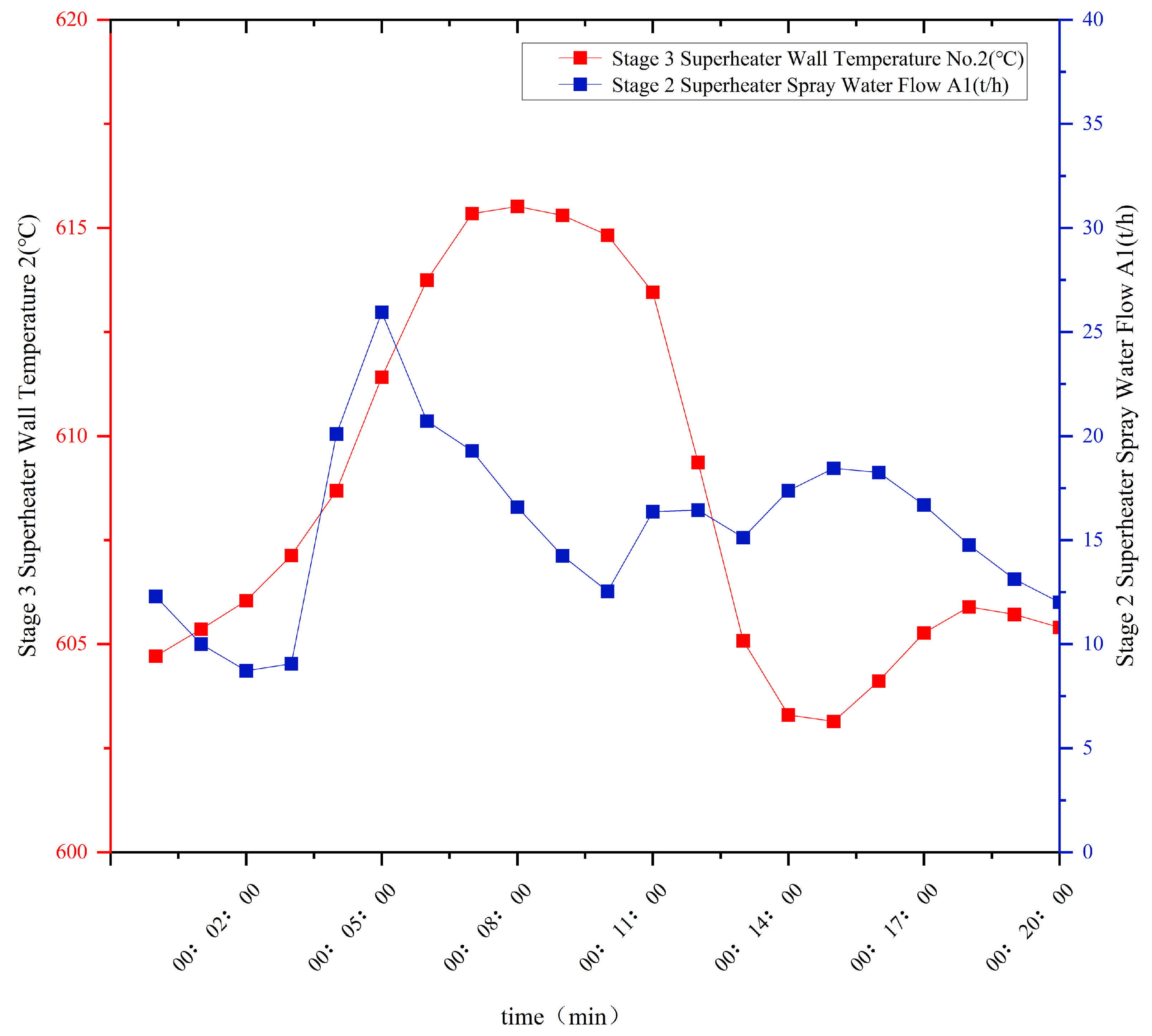
Figure 2 illustrates the response characteristics of the wall temperature at Measurement Point No. 2 of the tertiary (high-temperature) superheater to variations in the secondary desuperheater spray water flow. Stage 3 Superheater Wall Temperature No. 2 (°C) refers to the wall temperature measured at the second measurement point on the left side of the Stage-3 superheater, while Stage 2 Superheater Spray Water Flow A1 (t/h) represents the spray water flow measured at the first left-side point of the Stage-2 desuperheater. It can be observed that the spray flow rate increased at the 4th minute. Subsequently, at approximately the 9th minute, the wall temperature at Measurement Point No. 2 began to decrease, indicating a response lag of around 5 min (300 s). Therefore, to ensure sufficient time to implement cooling measures, it is necessary to predict the wall temperature of the high-temperature superheater at least 5 min in advance.
Given the complexity of the thermal power plant environment and the susceptibility of signal acquisition to noise interference, the large volume of raw data inevitably contains missing and abnormal values. Prior to data analysis, the raw dataset was preprocessed using techniques such as missing value imputation and duplicate value removal. Specifically, for missing and anomalous data points, a linear interpolation method in the time domain was applied to ensure the completeness and consistency of the dataset.

3. Methodology

3.1. Random Forest-Based Data Dimension Reduction

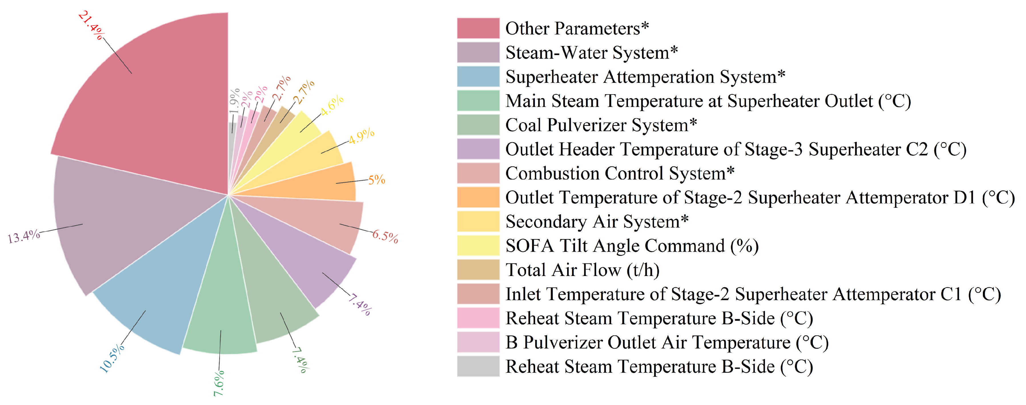
Based on the historical dataset, 106 primary parameters potentially affecting superheater wall temperature were evaluated, including load, fuel and air flows, feedwater flow, burner swing commands, damper positions, and steam parameters. The Random Forest (RF) algorithm was applied to calculate feature importance scores, and 68 key variables were selected, accounting for 95% of the cumulative importance. The feature importance results are shown in Figure 3, a rose chart displaying the top nine variables individually and the rest grouped by category, with an asterisk (*) denoting merged categories.
According to the analysis, the Steam–Water System (13.4%) and the Superheater Attemperation System (10.5%) exhibited the highest importance, reflecting the dominant role of steam-side cooling and spray attemperation in regulating wall temperature. On the gas side, the Main Steam Temperature at the superheater outlet (7.6%) and the Stage-3 Superheater Outlet Header Temperature C2 (7.4%, i.e., the outlet header temperature at the second position on the left side of the Stage-3 superheater) directly characterize the thermal load of the heating surface and show a clear positive correlation with wall temperature. Meanwhile, the Outlet Temperature of the Stage-2 Attemperator D1 (5%, the outlet temperature of the first desuperheater on the right side) and the Inlet Temperature of Stage-2 Superheater Attemperator C1 (2.7%, the inlet temperature of the first desuperheater on the left side) reflect the effectiveness of spray water mixing, where higher spray flow leads to a reduction in wall temperature.
Combustion-related variables also contributed significantly. The Coal Pulverizer System (7.6%) and the B Pulverizer Outlet Air Temperature (2%) influence coal drying and ignition stability, thereby affecting flame intensity and heat transfer. The SOFA Tilt Angle Command (4.6%) and the Secondary Air System (4.9%) regulate flame shape and spatial distribution, improper tilt or secondary air allocation may induce local overheating and raise wall temperature. Finally, the Total Air Flow (2.7%) is closely linked to load, under constant fuel input, excessive air supply reduces flame temperature and suppresses wall temperature rise.

3.2. Sliding Window Extraction

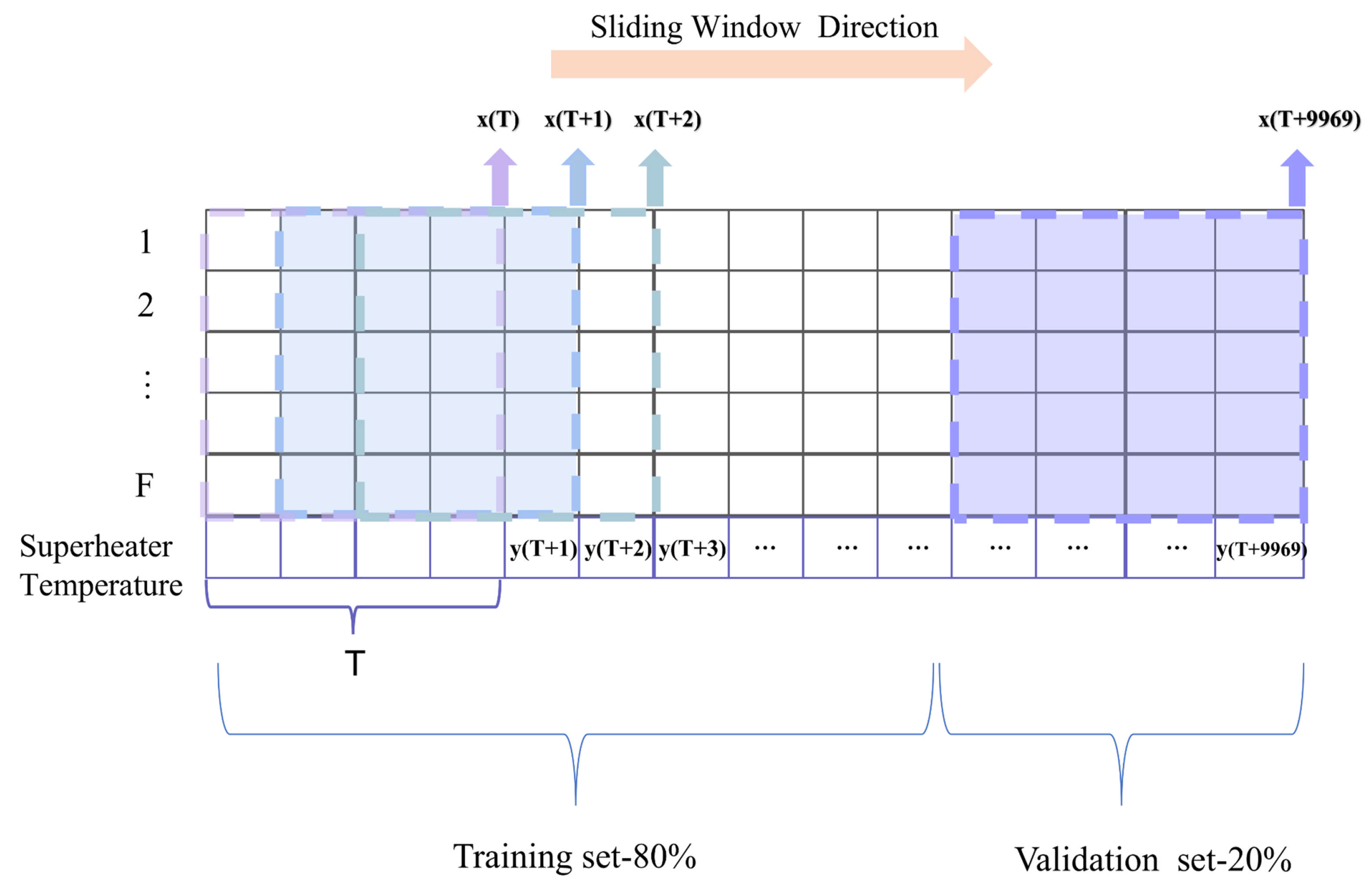
To effectively capture temporal dependencies embedded in long multivariate time series, a sliding window strategy is adopted to segment the raw sequence into fixed-length input units. As illustrated in Figure 4 the original sequence is partitioned into a set of overlapping (or non-overlapping) subsequences using a window of length T and stride S. Each resulting segment consists of T consecutive time steps and serves as an independent input sample for the model. The process is formalized in Table 1, which presents the pseudo-code for constructing the dataset via the sliding window mechanism. Each generated sample is organized into a three-dimensional tensor X B × F × T , where B denotes the batch size (i.e., the number of samples in one training batch), F represents the feature dimensionality, T is the time window length (number of time steps per sample). This window-based transformation enables the model to learn localized temporal dynamics while supporting efficient batch training.
Given an input sequence of total length L, the number of generated subsequences P can be calculated as Equation (1).
P = L T S + 1

3.3. MLPs

Multilayer Perceptrons (MLPs), a class of feedforward artificial neural networks, are inspired by biological neuronal information processing [18]. Early perceptron models [19] achieved binary classification via weighted summation and nonlinear activation functions, but their linear single-layer structure limited modeling of XOR and nonlinear relationships. MLPs address this by stacking multiple neuron layers with nonlinear activations, forming a hierarchical feature transformation architecture.
An MLPs consist of an input layer, hidden layers, and an output layer. The input layer transmits data to hidden layers where activation functions transform inputs. Stacking hidden layers extracts increasingly abstract features, while the output layer generates predictions. This process relies on two key components:
First, the fully connected structure, where each node (neuron) in a layer connects to all outputs from the previous layer, endows MLPs with strong feature representation capabilities. For a single node in a given layer, this process can be expressed as follows:
S j = f ( i = 1 n ( W i j X i ) B j ) ,     j = 1 , 2 , , h ,
where f denotes the activation function, n represents the number of nodes in the previous layer, W i j indicates the connection weight from the i-th node of the previous layer to the j-th node of the current layer, B j is the bias term for the j-th node in this layer, X i signifies the i-th input value, S j denotes the output value of the j-th node in the current layer, and h represents the total number of nodes in this layer.
Second, the nonlinear activation function, which breaks the linear constraints of multi-layer stacking and enables the network to express complex mapping relationships between inputs and outputs. There are various types of activation functions, with commonly used examples including Sigmoid, Tanh, and ReLU functions that can be expressed as follows:
f ( x ) = sigmoid ( x ) = 1 1 + e x
f ( x ) = Tanh ( x ) = e x e x e x + e x
f ( x ) = Re LU = max ( 0 , x )
where x denotes the input value to the activation function and f(x) represents the transformed output.
The Universal Approximation Theorem [20,21] establishes MLPs as universal function approximators: a single hidden layer with sufficient neurons can approximate any continuous function on compact sets. By adjusting network architectures and parameters, MLPs can be adapted to various problems, delivering accurate predictions and decisions. During practical training, the backpropagation algorithm [22], can be employed to efficiently compute gradients of the loss function with respect to parameters through chain rule, enabling end-to-end training when combined with gradient descent optimization.
In CNN architecture, MLP, with its fully connected property, undertakes the critical role of high-level feature decoding and decision generation. Classic models such as AlexNet [23], VGGNet [24] and ResNet [25] all adopt a unified paradigm, where convolutional layers extract spatial local features, pooling layers achieve dimensionality reduction and translation invariance, and finally, the flattened feature vector is fed into the fully connected layers of MLP to integrate global feature information and output prediction results. In the energy field, this architecture is widely utilized: Wang et al. [26] applied a Channel Selection CNN (CS-CNN) to predict boiler thermal efficiency, NOx emissions, and wall temperature under variable loads, while Chen et al. [27] developed a WGCN-GRU model for boiler heating surface temperature forecasting.
However, the fully connected nature of MLP has several limitations: First, the number of parameters increases quadratically with the input dimension, leading to significant computational and storage overhead, Second, the dense connectivity of the weight matrix renders the function mapping process a “black-box” characteristic, making it difficult to trace the contribution paths of features, Lastly, although universal approximation holds, an extremely large network scale may be required to accurately fit specific function structures, such as high-frequency oscillations or sparse features. These limitations motivate researchers to explore alternative architectures with greater parameter efficiency and interpretability.

3.4. Kolmogorov Arnold Networks

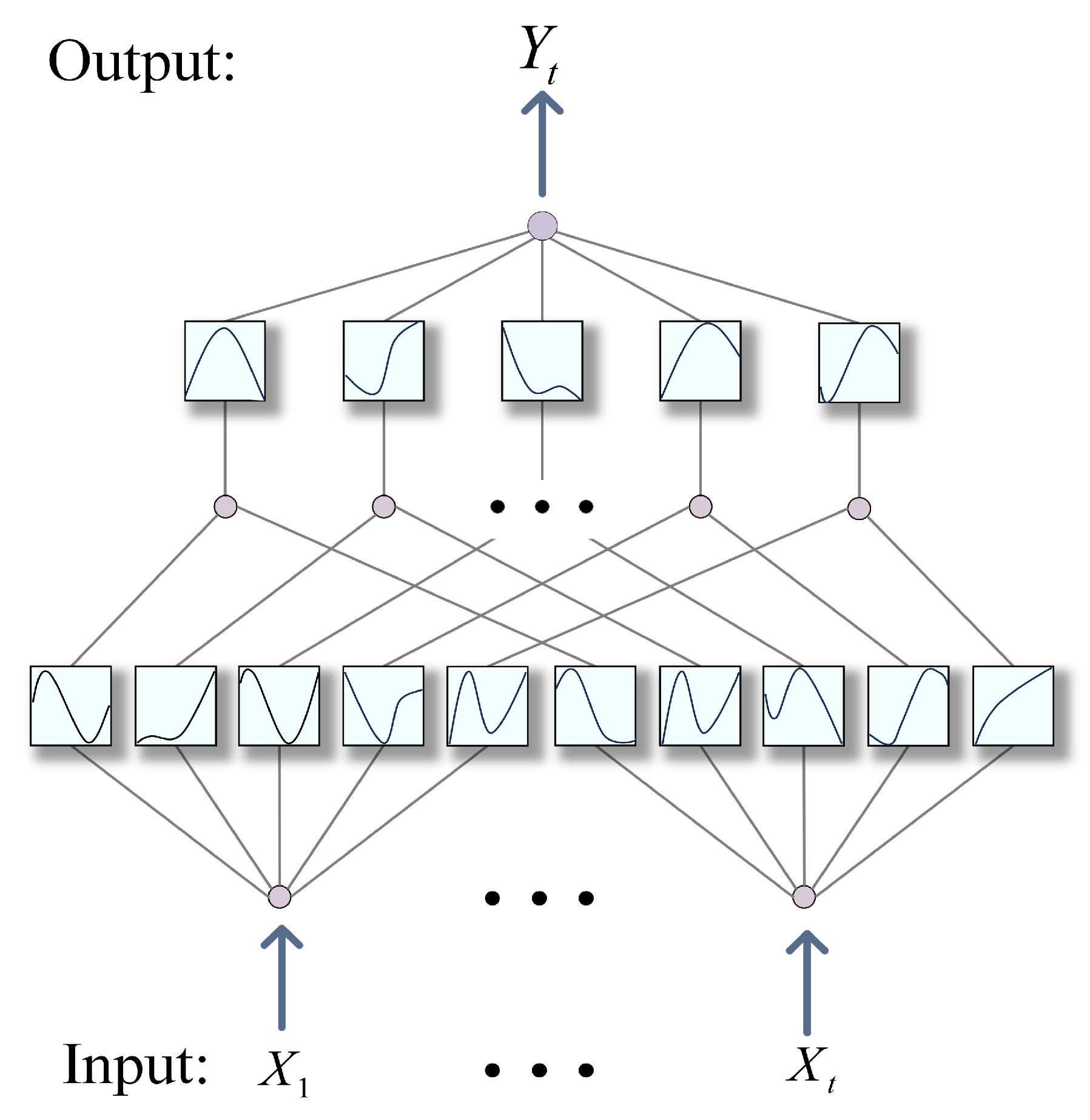
Kolmogorov Arnold Network (KAN) is a new type of neural network proposed by Liu et al. [28] in 2024, which can serve as promising alternatives to Multi-Layer Perceptrons (MLPs). Like MLPs, KANs have fully connected structures. However, whereas MLPs have fixed activation functions on nodes, KANs place learnable activation functions on edges.
Unlike MLPs which utilize the universal approximation theorem, KANs are fundamentally based on the Kolmogorov-Arnold theorem. This theorem states that any continuous function defined on a closed n-dimensional interval can be represented by the composition and summation of a finite number of one-dimensional continuous functions. A typical schematic diagram of the model is shown in Figure 5. More specifically, for a continuous f: [ 0 , 1 ] n ,
f ( x ) = f ( x 1 , , x n ) = q = 1 2 n + 1 Φ q p = 1 n ϕ q , p ( x p ) ,
where x = ( x 1 , x 2 , , x n ) denotes the input vector, n represents the input dimensionality, ϕ q , p : [ 0 , 1 ] are the inner one-dimensional continuous functions applied to individual input components, and Φ q : are the outer one-dimensional continuous functions that combine the inner outputs. Inspired by MLPs, KAN layers can be defined with n i n -dimensional inputs and n o u t -dimensional outputs. The Kolmogorov-Arnold representations in Equation (6) are simply compositions of two KAN layers, the inner functions form a KAN layer with n in =   n and n out =   2 n + 1 , and the outer functions form a KAN layer with n in =   2 n + 1 and n out =   1 . However, such a two-layer-network is too simple to approximate any function arbitrarily well in practice with smooth splines. So, we stack more KAN layers, and the output of KAN is
KAN ( x ) = ( Φ L 1 Φ L 2 Φ 1 Φ 0 ) x
Each KAN layer can be represented as a matrix of one-dimensional functions:
Φ l = { ϕ l , q , p } , p = 1 , 2 , , n in , q = 1 , 2 , , n out
The transformation Φ l of each layer operates on the input x l to generate the input x l + 1 for the next layer, which can be described as follows:
x l + 1 = ϕ l , 1 , 1 ( ) ϕ l , 1 , 2 ( ) ϕ l , 1 , n l ( ) ϕ l , 2 , 1 ( ) ϕ l , 2 , 2 ( ) ϕ l , 2 , n l ( ) ϕ l , n l + 1 , 1 ( ) ϕ l , n l + 1 , 2 ( ) ϕ l , n l + 1 , n l ( ) Φ l x l
where n l is the number of nodes in the ith layer of the computational graph. Additionally, since all functions ϕ l , q , p in this matrix are univariate functions, we can parametrize each 1D function as a B-spline curve, with learnable coefficients of local B-spline basis functions:
ϕ ( x ) = w b b ( x ) + w s spline ( x )
The b ( x ) is a basis function which is similar to residual connections. In most cases, it can be set as follows:
b ( x ) = silu ( x ) = x / ( 1 + e x )
And spline ( x ) is parametrized as a linear combination of B-splines such that
spline ( x ) = i c i B i ( x )
where c i are trainable.
With their unique architectural design, KANs effectively capture complex nonlinear relationships in data and typically require much smaller computation graphs than MLPs. In terms of accuracy, compact KANs achieve comparable or superior performance relative to larger MLPs in function fitting tasks. Regarding interpretability, KANs offer intuitive visualization and facilitate seamless human interaction. While MLPs may learn generalized additive structures, they prove highly inefficient for approximating exponential and sinusoidal functions when using ReLU activations. In contrast, KANs excel at learning both compositional structures and univariate functions, demonstrating significant advantages over MLPs.

3.5. PLO

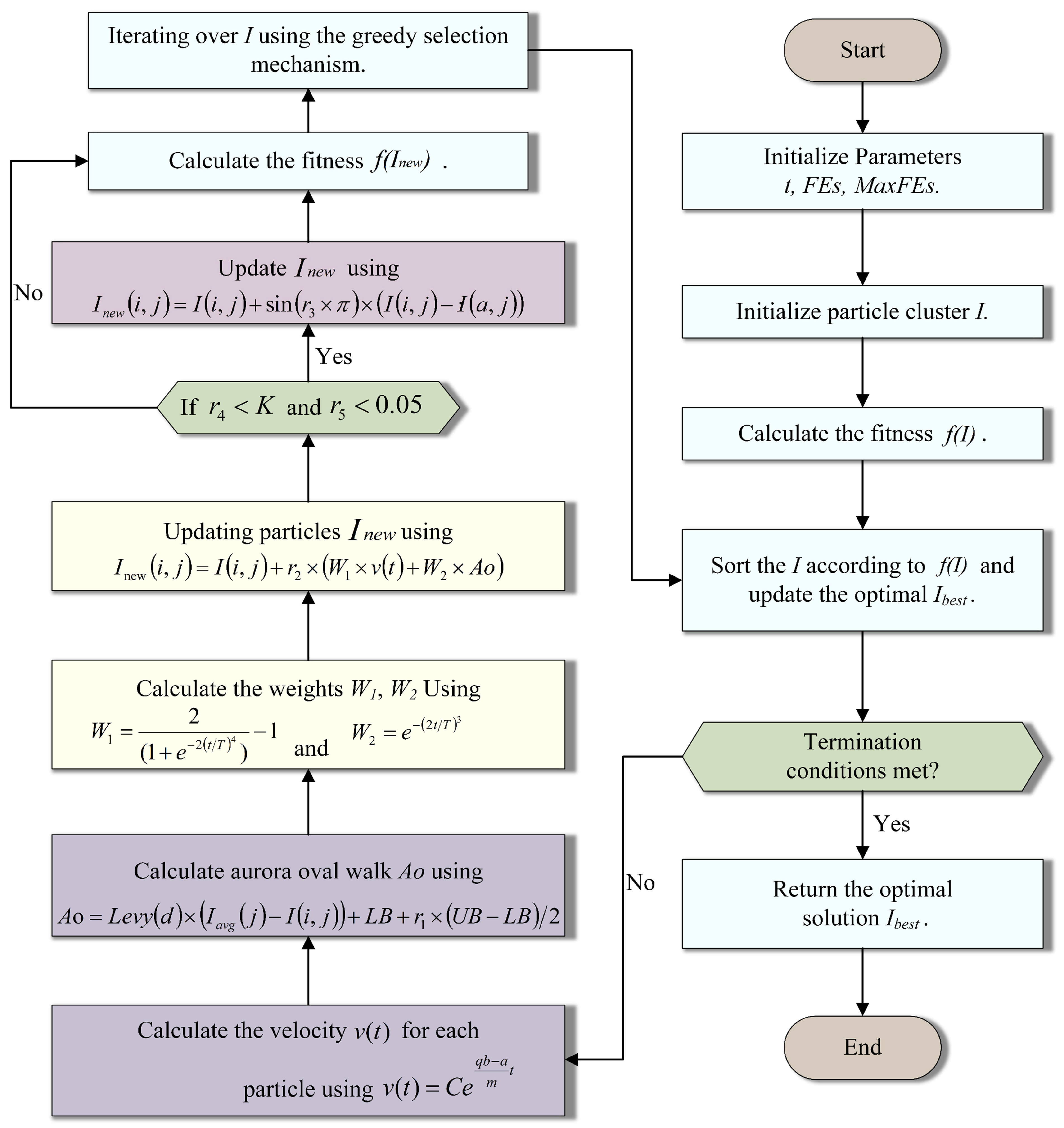
The Polar Lights Optimization (PLO) algorithm is a metaheuristic optimization method inspired by the natural phenomenon of auroras, which is proposed by Yuan et al. in 2024 [29]. In PLO, the gyration motion is proposed through the motion process of energetic charged particles spiraling forward around magnetic lines of inductance, then, the aurora oval walk is proposed by synthesizing the energies, velocities, and trajectories of charged particles, as well as the compositions and conditions in the atmosphere, where auroras present an elliptical luminous ring belt in the sky. Finally, the particle collision strategy is proposed through the phenomenon of energetic charged particles colliding with one another continuously on their flights. The flow of the algorithm is shown in Figure 6. The fundamental principles of this algorithm are described as follows:
  • Step 1. Initialization phase
The population consists of N candidate solutions, where N represents the population size, and each solution is defined in a D-dimensional solution space, with D denoting the scalable dimension. The entire population is represented as a matrix, initialized as follows:
I ( N , D ) = L B + R × ( U B L B ) = I ( 1 , 1 ) I ( 1 , 2 ) I ( 1 , D ) I ( 2 , 1 ) I ( 2 , 2 ) I ( 2 , D ) I ( N , 1 ) I ( N , 2 ) I ( N , D ) ,
where U B and   L B denote the boundaries of the solution space, and R denotes a random number sequence that takes values in [0, 1]. In PLO, the motion of energetic charged particles toward Earth’s polar via the magnetic susceptor is simulated using a search agent in solution space.
  • Step 2. Gyration motion:
When charged particles approach the Earth, the Lorentz force exerts a centripetal effect on charged particles, causing them to undergo gyration along magnetic field lines. The kinetic equation of the charged particles is described as follows:
m d v d t = q v B
where m is the mass of a charged particle, q is the particle charge, v is the velocity vector, B the magnetic-field magnitude. However, these high-energy particles are subjected to air molecular drag in the atmosphere, resulting in non-smooth circular motion and causing a gradual decrease in the radius of the particle’s circular motion. By incorporating this damping phenomenon into the governing equation describing the temporal evolution of particle velocity, the Equation (14) for charged particle velocity can be modified as follows:
m d v d t = q v B α v
Then solving this differential equation, we obtain the following:
v ( t ) = C e q B α m t
where C is the integration constant. For simplicity, this strategy sets C , q , and B to 1, with m assigned a value of 100. The damping factor α is a random value within the interval [1, 1.5], and the algorithm simulates the temporal evolution of variable t in Equation (16) through a fitness evaluation process.
  • Step 3. Aurora oval walk:
The auroral oval walk in PLO helps to search the solution space efficiently. Astronomical studies of auroral phenomena reveal that auroras typically form along a band-shaped region known as the auroral oval. The size of the auroral oval depends on the north–south component of the interplanetary magnetic field, with its boundaries varying according to geomagnetic activity intensity. Earth’s complex atmospheric structure further influences the trajectories of various high-energy particles involved in this phenomenon.
The intricate fluctuating characteristics of auroral oval wandering exhibit significant impacts on global search, and this unpredictable chaotic property precisely meets the PLO algorithm’s requirement for rapid global exploration of the solution space. Levy Flight (LF) is commonly used in metaheuristic algorithms to boost global exploration due to its random non-Gaussian walk nature. Step values follow the Levy stable distribution, expressed in Equation (17) as:
L e v y ( d ) | d | 1 β , 0 < β 2
where β is an adjustment stability index and d is the step size. In the auroral oval walk, the energetic particles simulated with LF are affected by geomagnetic activity and atmosphere, exhibit auroral oval boundary contraction in polar regions and expansion in equatorial regions. The specific change process is shown in Equation (18):
A o = L e v y ( d ) × ( I a v g ( j ) I ( i , j ) ) + L B + r 1 × ( U B L B ) / 2
where A o is the complex variation in the auroral oval simulated through dispersed distribution of the LFs, which drives energetic particles to move between polar regions and the equator. I a v g denotes the mass center position of the energetic particle swarm, which is calculated by
I avg = 1 N × i = 1 N I ( i )
and I ( i , j ) represents the current position of the energetic particle, while I a v g ( j ) I ( i , j ) characterizes the particle’s movement tendency.
The PLO algorithm incorporates two primary motion patterns during the search process: gyration motion and auroral oval walk. The gyration motion emphasizes local exploitation and fine-tuning, aiming to thoroughly explore local solution spaces to find local optima or refining the local structure of current solutions. In contrast, the auroral oval walk focuses on global exploration characteristics, where particles investigate the solution space with larger step sizes to discover more valuable regions. By integrating these two strategies, the proposed computational model is presented in Equation (20):
I new ( i , j ) = I ( i , j ) + r 2 × ( W 1 × v ( t ) + W 2 × A o )
where I new ( i , j ) denotes the position of energetic particles after renewal, and r 2 represents the disturbance caused by uncontrollable environmental factors with a value range of [0, 1]. Additionally, we introduce adaptive weight W 1 and W 2 that vary with algorithm iterations to maximize the efficiency of both local exploitation and global exploration during the optimization process, whose calculation formulas are given in Equations (21) and (22):
W 1 = 2 ( 1 + e 2 ( t / T ) 4 ) 1
W 2 = e ( 2 t / T ) 3
As the algorithm iterates, global search and local exploitation achieve balance through these dynamically changing weight adjustments, thereby facilitating the exploration of the optimal solution.
  • Step 4. Particle collision:
To enhance the algorithm’s capability for avoiding or escaping local optima, PLO incorporates a particle collision strategy. In this mechanism, the currently moving particle may undergo chaotic collisions with any particle in the swarm, thereby altering its velocity and direction to disperse into different regions. The representation is as follows:
I n e w ( i , j ) = I ( i , j ) + sin ( r 3 × π ) × ( I ( i , j ) I ( a , j ) ) , r 4 < K ,   r 5 < 0.05
where I ( a , j ) represents any particle in the particle cluster, r 3 and r 4 are random values, taking values in [0, 1]. Collisions between particles become more frequent as the algorithm proceeds and are therefore controlled by the collision probability K , calculated by Equation (24):
K = ( t / T )

3.6. KAN Model Hyperparameter Optimization

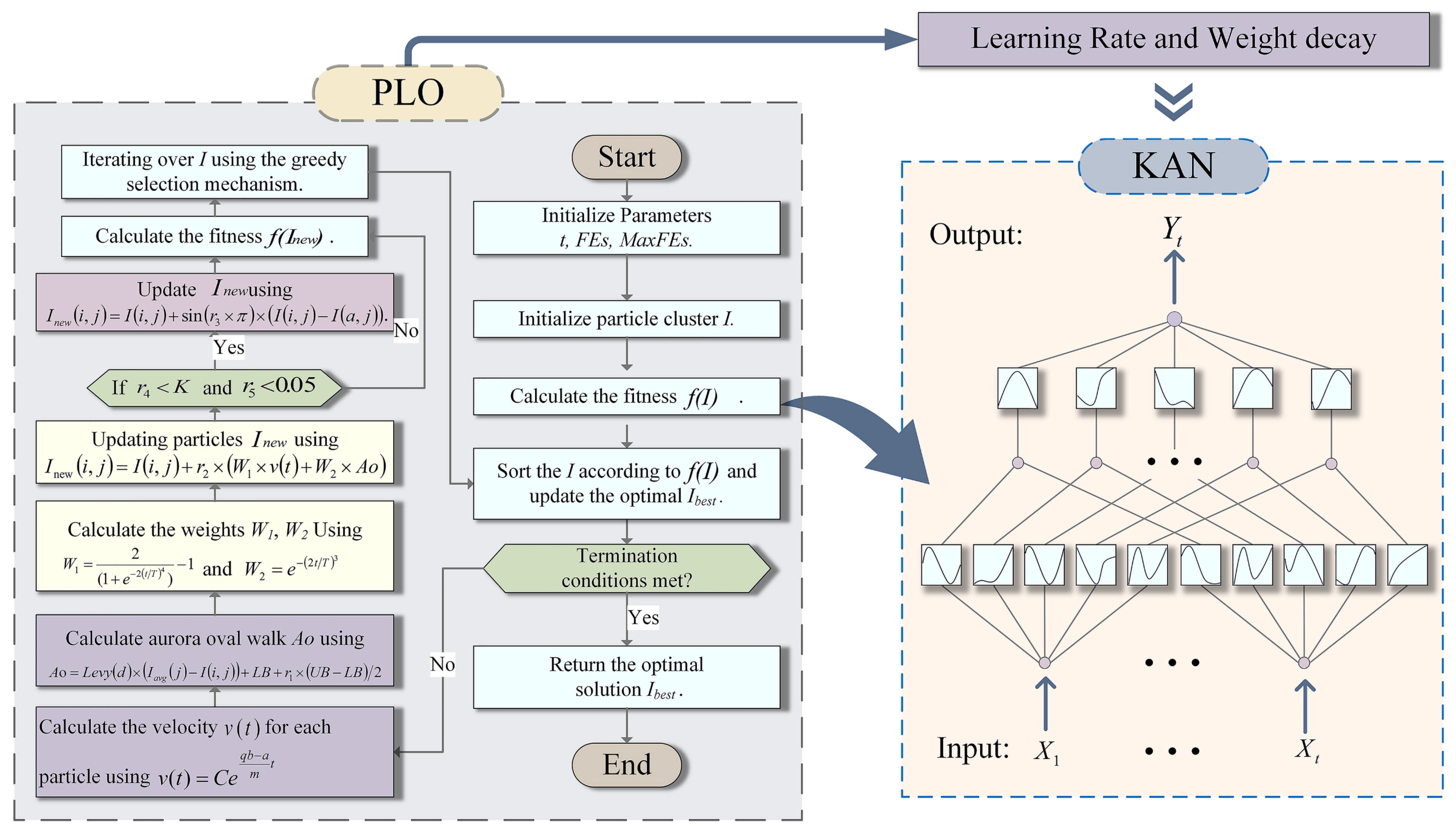
To optimize the performance of the KAN model, the width and depth were determined through preliminary grid search experiments. Subsequently, the Adam optimizer’s hyperparameters, learning rate and weight decay, were optimized using the Polar Lights Optimization (PLO) algorithm. The operational data from an in-service ultra-supercritical variable-pressure once-through boiler was used for validation, with 10,000 samples collected over one week at 60 s intervals, focusing on the high-temperature superheater’s elevated wall temperature across varying load conditions. A 5 min (300 s) prediction horizon was set to account for the response delay between desuperheating spray adjustments and wall temperature variations, with 80% of the data used for training and 20% for validation. The PLO algorithm’s hyperparameter search ranges were defined as follows: learning rate in [0.001, 0.1] and weight decay in [1 × 10⁻⁵, 1 × 10⁻³]. The flowchart of the KAN model optimized by PLO is shown in Figure 7. The following are the detailed steps and formulas for optimizing the PLO algorithm.
  • Step 1. Define the hyperparameter space
For the KAN model, the search space for the Adam optimizer’s hyperparameters is defined as
Θ = { l r , w d }
where lr denotes the learning rate and wd denotes the weight decay.
  • Step 2. Initialize the auroral particles.
Auroral particles are randomly generated in the hyperparameter search space with initial positions X 0 i and light intensity values I 0 i . Each particle represents a set of hyperparameter combinations for the KAN model.
  • Step 3. Define the fitness function.
The model is trained under each set of hyperparameters, and the fitness value is calculated to evaluate performance. The fitness function is defined as the mean squared error (MSE) of the predicted superheater wall temperature:
F i t = 1 T t = 1 T ( T t T t ) 2
where T is the total number of samples, T t is the predicted wall temperature, and T t is the true wall temperature.
  • Step 4. Update the particle positions.
The position of each particle is updated according to the PLO algorithm’s dynamic rule, incorporating gyration motion for local exploitation and aurora oval walk for global exploration. Specifically, Equation (16) with q = 1 , B = 1 , m = 100 , and damping factor α [ 1 , 1.5 ] models gyration motion, and Equation (18) with r 2 [ 0 , 1 ] represents the aurora oval walk.
  • Step 5. Calculate the light intensities of the particles.
The light intensity value of each particle is calculated based on its new position:
I k + 1 i = F i t ( X k + 1 i )
The light intensity reflects the model’s performance for the current hyperparameter configuration.
  • Step 6. Particle collision.
To escape local optima, a particle collision strategy is applied, which can be expressed as Equation (23) with r 3 , r 4 [ 0 , 0.05 ] .
  • Step 7. Update the individual and global optimal positions.
The current light intensity of each particle is compared with its historical best. If the current value is better, the individual optimal position is updated. The global optimal position is updated by selecting the particle with the best light intensity among all particles.
  • Step 8. Check the iteration termination condition.
If the termination condition is met, the algorithm stops, otherwise, it returns to Step 4.
  • Step 9. Train the model.
Using the optimal hyperparameter combination obtained via PLO, the KAN model is constructed and trained.
  • Step 10. Test the model performance.
The optimized KAN model is applied to the test set, and the model error is evaluated.

3.7. Research Framework

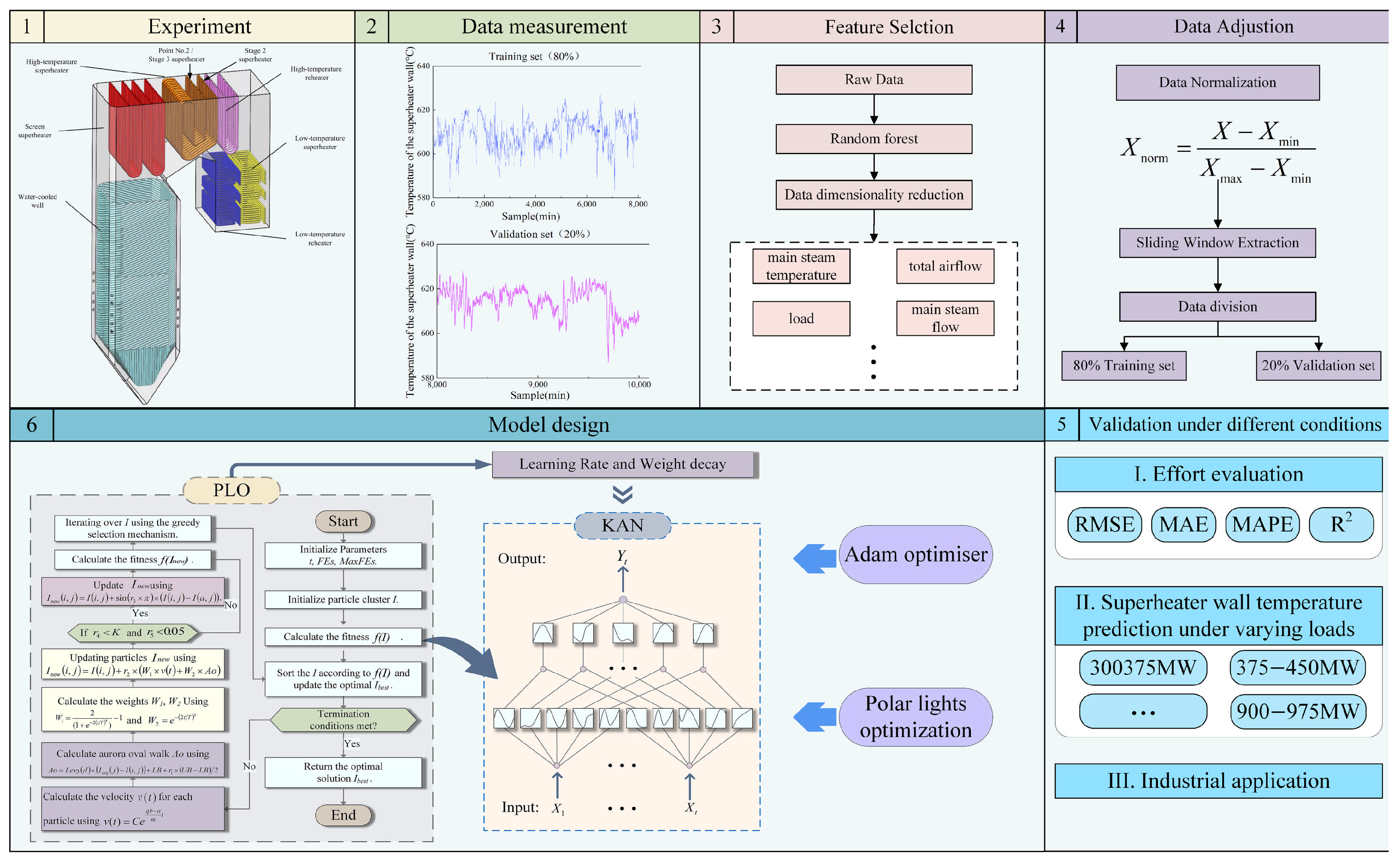
In this study, a high-precision high-temperature superheater wall temperature model is introduced on the basis of the PLO-optimized Kolmogorov Arnold network. The framework includes five core aspects: experimental design, feature selection, sliding window extraction, model design and model validation, as shown in Figure 8. For experimental design, this study utilizes operational data from an in-service ultra-supercritical variable-pressure once-through boiler. The selected measurement points on the high-temperature superheater consistently exhibited elevated wall temperature across varying load conditions. A total of 10,000 samples were collected over a one-week period with a 60 s interval. Due to the observed response delay between desuperheating spray adjustments and wall temperature variations, a minimum prediction horizon of 5 min (300 s) was determined to be necessary for effective thermal management. Given the complexity of the thermal power plant environment and the susceptibility to noise interference, the raw dataset was preprocessed to ensure quality. This involved duplicate value elimination and linear interpolation in the time domain to handle missing or anomalous data. All features were then scaled to the range [0, 1] using min–max normalization to avoid bias caused by differing data magnitudes. Feature selection was performed using the Random Forest algorithm on 106 candidate variables, resulting in 68 key features that capture the majority of input relevance. To incorporate temporal characteristics, a sliding window mechanism with a window size of T = 30 was employed, constructing each sample as a sequence of 30 time steps across the selected features. This transformation enables the model to learn dynamic patterns from the raw time-series data. For model design, a Kolmogorov Arnold Network (KAN) was employed to model the complex nonlinear mapping between input features and the target variable. Unlike traditional MLPs, KAN introduces learnable B-spline activation functions on edges, enabling more compact and interpretable representations. The layered structure efficiently captures data patterns while maintaining model transparency. The width and depth of the KAN model were determined through preliminary grid search experiments. Subsequently, the learning rate and weight decay of the Adam optimizer were optimized using the Polar Lights Optimization (PLO) algorithm, which balances local exploitation (gyration), global exploration (aurora oval walk), and local optima escape (particle collision) through adaptive weighting. Dropout regularization further enhances training stability and generalization. In the model validation stage, comprehensive evaluation was performed using MAE, MSE, RMSE, MAPE, and R2 metrics. The proposed KAN-PLO model was benchmarked against classical MLP models. Results demonstrated superior accuracy, robustness, and predictive stability of the proposed framework under dynamic thermal conditions, verifying its effectiveness in real-world plant scenarios.

4. Analysis of Experimental Process and Results

First, the model input data are standardized via Z-score normalization. Next, the window size is set to 30 and the stride to 1, after which a sliding window is applied along the temporal dimension of the original long-term sequence. This process continues until the window has traversed the entire time series, yielding 9970 subsequences. The forecast target for each subsequence is defined by the prediction step size. The forecast target for each subsequence is defined by the prediction step size. Specifically, the first forecast corresponds to the superheater wall temperature at the next time step following the end of the current window (i.e., at Measurement Point No. 2). Subsequent predictions are generated sequentially according to the specified step size.
During the experiment, the preprocessed subsequences are split with an 80:20 ratio, yielding 7976 samples for training and 1994 samples for testing. The proposed KAN model is trained on the training set within the PyTorch framework (Python 3.10, PyTorch 2.4.0+cu124, NumPy 1.26.4). All experiments were conducted on a system with an AMD Ryzen 9 8945HS CPU, 32 GB RAM, and an 8 GB GPU, running Windows 11. Model performance is evaluated using four metrics: mean absolute percentage error (MAPE), root mean square error (RMSE), mean absolute error (MAE), and coefficient of determination (R2), defined as follows:
M A P E = 1 n i = 1 n y i y i ^ y i 100 %
R M S E = 1 n i = 1 n ( y i y i ^ ) 2
M A E = 1 n i = 1 n y i y i ^ × 100 %
R 2 = 1 i = 1 n ( y i y i ^ ) 2 i = 1 n ( y i y i ¯ ) 2
In these formulas, y i , y ^ i , y ¯ i represents the average of the actual measured value, the predicted value, and the mean of the actual values, and n is the total number of samples.

4.1. Structural Analysis: The Effect of Width and Depth on Model Performance

4.1.1. Consistent Hyperparameter Configuration

To ensure the validity and comparability of results across different network structures, we fixed the following key hyperparameters throughout all experiments. This guarantees that only the network width and depth differ between configurations:
Step 1: Grid size was set to 5, and spline order was fixed at 3 (i.e., cubic B-splines),
Step 2: Scaling noise was set to 0.1, both base scale and spline scale were set to 1.0,
Step 3: The option for standalone spline scaling was enabled to allow adaptive scaling per edge,
Step 4: The activation function was set to SiLU (Sigmoid Linear Unit),
Step 5: The grid range was kept within [−1, 1], and the grid perturbation step was set to 0.02,
Step 6: Input and output feature dimensions were determined by the dataset and task,
Step 7: All training hyperparameters—learning rate, optimizer (Adam), batch size, number of epochs, and random seed—were kept identical.

4.1.2. Canonical KAN Structure and Its Generalization

The canonical Kolmogorov–Arnold Network (KAN) structure for an input of dimension n is defined by Equation (6), to explore the structural flexibility of KAN, we generalize this architecture to allow arbitrary depth and width:
n , w 1 , w 2 , , w d , target_size
where d denotes the number of KAN layers (depth), and w i represents the number of nodes (composite functions) in the i -th hidden layer.

4.1.3. Experimental Design: Varying Width and Depth

We designed the experiments to investigate the structural sensitivity of KANs along two dimensions—width and depth—while keeping other hyperparameters constant. In KANs, “depth” is defined as the number of KAN layers, where each layer comprises a set of univariate spline transformations followed by additive aggregation. In this formulation, we generalize the architecture to support arbitrary depth and width. The target size is set to 1, and the number of node layers is defined as the number of KAN layers plus one.
(1)
Depth d = 1: Minimal Configuration Without Hidden Layer
In this configuration, the network includes only a single KAN layer that directly transforms the input features into the output, without any intermediate composite layer. The structure is denoted as:
[ n 1 ]
This setup corresponds to a depth-1 KAN, which learns n univariate spline functions and aggregates them linearly to produce the output. It serves as the minimal baseline and helps assess whether deeper or wider structures improve approximation in the current data context.
(2)
Depth d = 2 or 3: With Intermediate Composite Layers
When d 2 , the model contains at least one hidden KAN layer. The canonical KAN structure, grounded in the Kolmogorov–Arnold representation theorem, is realized at d = 2 , where the intermediate layer consists of exactly 2n + 1 univariate composite functions. To generalize this, we explore two width allocation strategies:
Progressive expansion (increasing width): Equation (33) ensuring that the final layer width matches the canonical 2n + 1.
w i = 2 n + 1 2 d 1 i , i = 1 , , d 1
Progressive reduction (decreasing width):
w i = 2 n + 1 2 i 1 , i = 1 , , d 1
Based on these, we construct the following architectures:
d = 2 :
w   =   2 n + 1
d = 3 , increasing:
w = 2 n + 1 2 , 2 n + 1
d = 3 , decreasing:
w = 2 n + 1 , 2 n + 1 2
Deeper configurations ( d 4 ) were not evaluated due to significantly increased training time and limited practical deploy ability.

4.1.4. Results and Structural Sensitivity Analysis

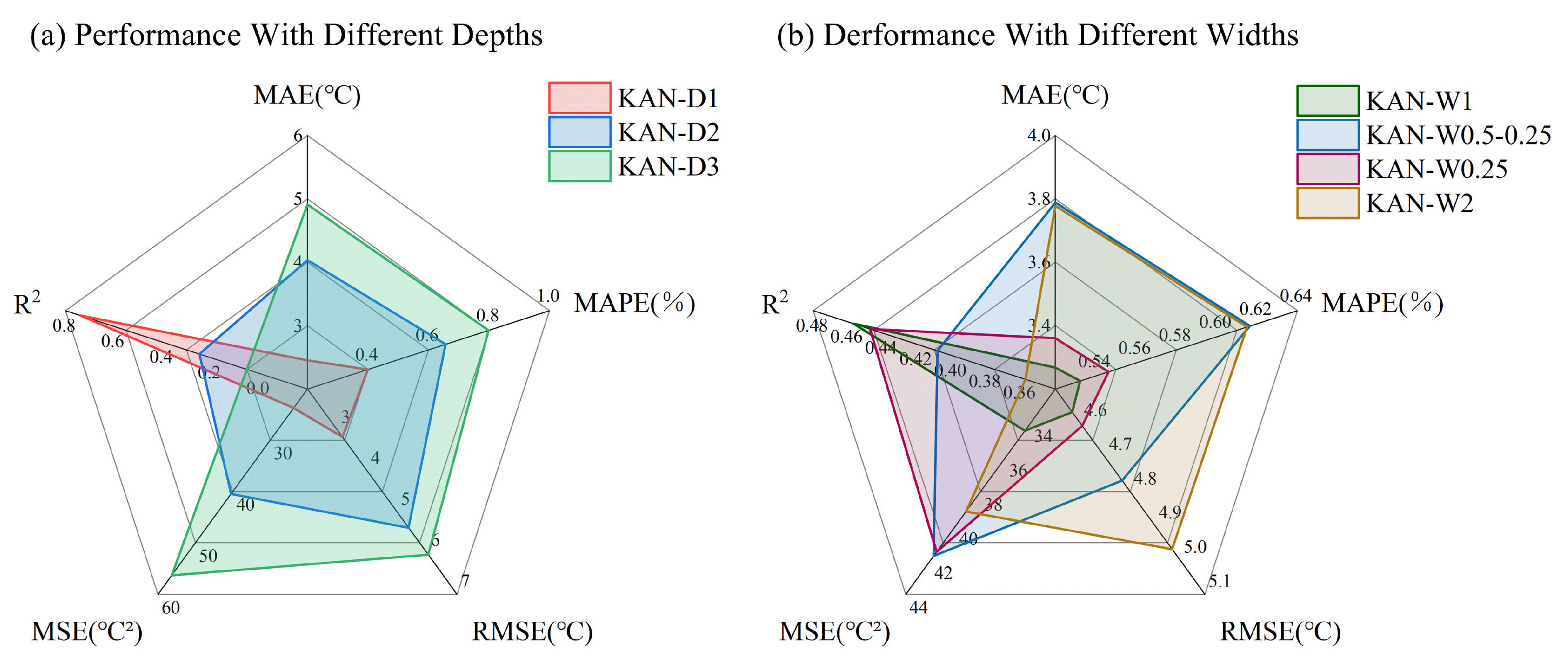
Quantitative results from all KAN architectures are visualized through radar and line plots, as shown in Figure 9. Figure 9a compares models with different depths, denoted as KAN-D1 (D1 type, no hidden layers), KAN-D2 (D2 type, canonical structure: input n → hidden layer 2n + 1 → output target size), and KAN-D3 (D3 type, i.e., KAN-W0.5-1, two hidden layers with widths of (2n + 1)/2 and (2n + 1)), using five performance metrics: mean absolute error (MAE), coefficient of determination ( R 2 ), mean absolute percentage error (MAPE), mean squared error (MSE), and root mean squared error (RMSE). Figure 9b presents models with varying layer widths under a fixed depth setting, where the canonical width is defined as (2n + 1), and width scaling factors are indicated in the legend: KAN-W1 (D2 type, width (2n + 1)), KAN-W0.25 (D2 type, width (2n + 1)/4), KAN-W2 (D2 type, width 2 × (2n + 1)), and KAN-W0.5-0.25 (D3 type, two hidden layers with widths of (2n + 1)/2 and (2n + 1)/4, respectively). Performance is evaluated using five metrics: MAE, R 2 , MAPE, MSE, and RMSE. In both subfigures, larger R2 values and smaller error metrics indicate better predictive performance, with the polygonal area in radar charts and line plots providing a visual summary of trade-offs across metrics.
From Figure 9a, KAN-D1 (D1 type, no hidden layers) achieves the best overall performance, surpassing KAN-D2 (D2 type) and KAN-D3 (D3 type, i.e., KAN-W0.5-1). The superior performance of KAN-D1 suggests that input features—processed through random forest-based selection and sliding time windows—already contain high-quality, temporally enriched information, rendering additional hidden layers potentially redundant. KAN-D2 performs next best, benefiting from the Kolmogorov–Arnold-prescribed width of 2n + 1, while KAN-D3 exhibits the poorest performance, indicating that deeper architectures cannot compensate for the feature engineering applied at the input level.
Figure 9b analyzes the performance of KAN models with varying layer widths under a fixed depth setting, where KAN-W1, KAN-W0.25, and KAN-W2 are of D2 type (single hidden layer), and KAN-W0.5-0.25 is of D3 type (two hidden layers). KAN-W1 (width (2n + 1)) demonstrates the strongest predictive performance, with higher R2 values and lower error metrics. KAN-W0.25 (width (2n + 1)/4) performs next best, followed by KAN-W2 (width 2 × (2n + 1)) and KAN-W0.5-0.25 (widths (2n + 1)/2 and (2n + 1)/4, respectively). KAN-W2 and KAN-W0.5-0.25 exhibit nearly equivalent performance but are outperformed by KAN-W1 and KAN-W0.25, suggesting that reducing width or excessively increasing width may lead to diminished approximation capability or redundancy. This reinforces the empirical advantage of the Kolmogorov–Arnold-prescribed width (2n + 1) in balancing computational complexity and predictive performance.

4.1.5. Summary and Insights

This study conducted a structural sensitivity analysis of KAN by independently varying depth and width under consistent spline, activation, and training settings. The key insights are:
(1)
The depth-1 configuration [ n 1 ] offers the best trade-off between simplicity and predictive accuracy, especially when the input features are already informative and temporally structured.
(2)
The canonical 2n + 1 width remains a stable and effective design choice when used as the final composite layer, validating theoretical expectations.
(3)
In deeper networks, progressive expansion of hidden layer widths yields better performance than decreasing-width strategies, though the marginal benefit is limited.
(4)
Overall, feature quality and preprocessing outweigh the gains from deeper or wider KAN architectures. Complexity should be introduced only when warranted by the data’s representational demands.

4.2. Hyperparameter Optimization—Polar Lights Optimizer

To enhance the prediction accuracy and fitting performance of the KAN model, the Adam optimizer was employed for model training, with the learning rate (lr) and weight decay coefficient optimized using the PLO algorithm. The search ranges were set to 0.001 ,   0.1 for lr and [ 1 × 10 5 , 1 × 10 3 ] for weight decay. In each iteration, five candidate solutions (particles) were generated, with each particle representing one combination of hyperparameters. Model training for each candidate was performed over 100 epochs, and the mean square error loss (MSELoss) on the validation set was used as the optimization objective. The optimization process was run for 30 iterations, allowing PLO to dynamically balance global exploration and local exploitation.
After convergence, the optimal hyperparameter configuration was determined as l r = 0.01 and weight_decay = 1 × 10 4 , achieving the lowest MSELoss of 23.6846 on the validation set. This configuration significantly outperformed other tested parameter sets, providing a more stable convergence and improved predictive accuracy. Table 2 presents the top 30 optimal hyperparameter configurations of the KAN model obtained by PLO, ranked in ascending order of MSELoss, offering a clear reference for parameter selection in different experimental settings.

4.3. Results and Discussions

This section evaluates the proposed KAN model using operational data from a 1000 MW ultra-supercritical primary reheat unit. The dataset comprises 10,000 samples from the Supervisory Information System (SIS) collected between 22 October and 29 October 2024, covering load intervals from 300 MW to 975 MW. Following Random Forest-based feature selection, 68 key variables were retained as model inputs. Measurement Point No. 2 on the wall of the high-temperature superheater was chosen as the prediction target due to its consistently elevated temperature across varying load conditions.

4.3.1. Comparative Analysis of Superheater Wall Temperature Prediction Performance Under Different Load Conditions

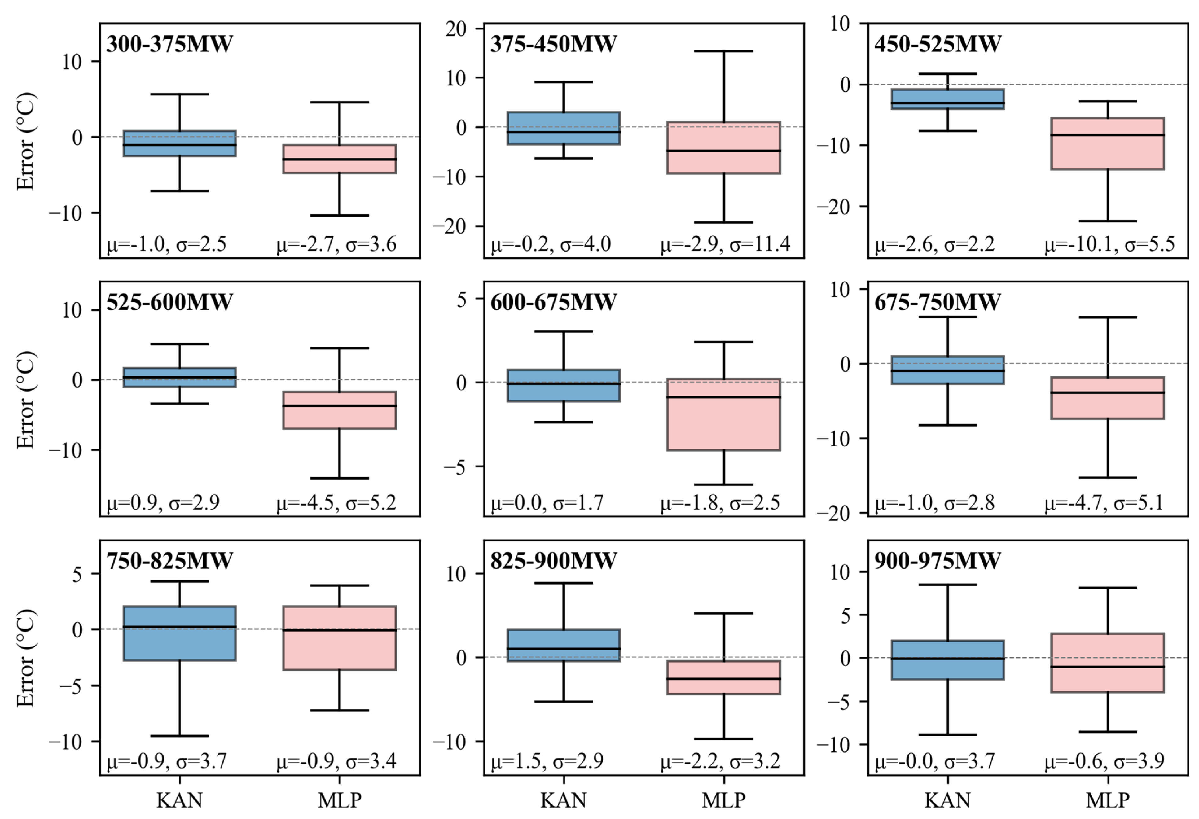
To evaluate the relative prediction accuracy of the proposed KAN model, a comparative analysis was conducted against a conventional MLP model using the experimental dataset described in Section 4.3. Figure 10 presents boxplots of prediction errors for both models across nine load bins. The KAN model consistently outperforms the MLP under low to medium load conditions, particularly in the 300–600 MW range. For example, at 450–525 MW, the KAN achieves a mean error (μ) of −2.628 °C and a standard deviation (σ) of 2.206 °C, compared to the MLP’s −10.098 °C and 5.504 °C. Similarly, at 525–600 MW, the KAN maintains a dispersion of 2.909 °C versus 5.217 °C for the MLP, indicating greater stability and noise tolerance. The performance gap is most pronounced at 375–450 MW and 675–750 MW, where the MLP’s error variance exceeds 5 °C, while the KAN remains below 3 °C.
In higher load ranges (750–975 MW), both models perform comparably in error magnitude, though the KAN generally achieves slightly better mean accuracy with similar variance. Notably, at 900–975 MW, the KAN’s μ   =   0.030   ° C and   σ   =   3.719   ° C closely match the MLP’s μ   =   0.611   ° C and σ   =   3.854   ° C . These results indicate that while both models sustain predictive performance under high-load conditions, the KAN offers markedly superior accuracy and robustness under low-load scenarios, where operating conditions fluctuate more sharply and data sparsity can challenge generalization.
In summary, the KAN demonstrates lower error bias and variance across most load bins, particularly under low and medium loads, confirming its potential for more reliable and stable wall temperature prediction in real-world boiler operations.

4.3.2. Industrial Application

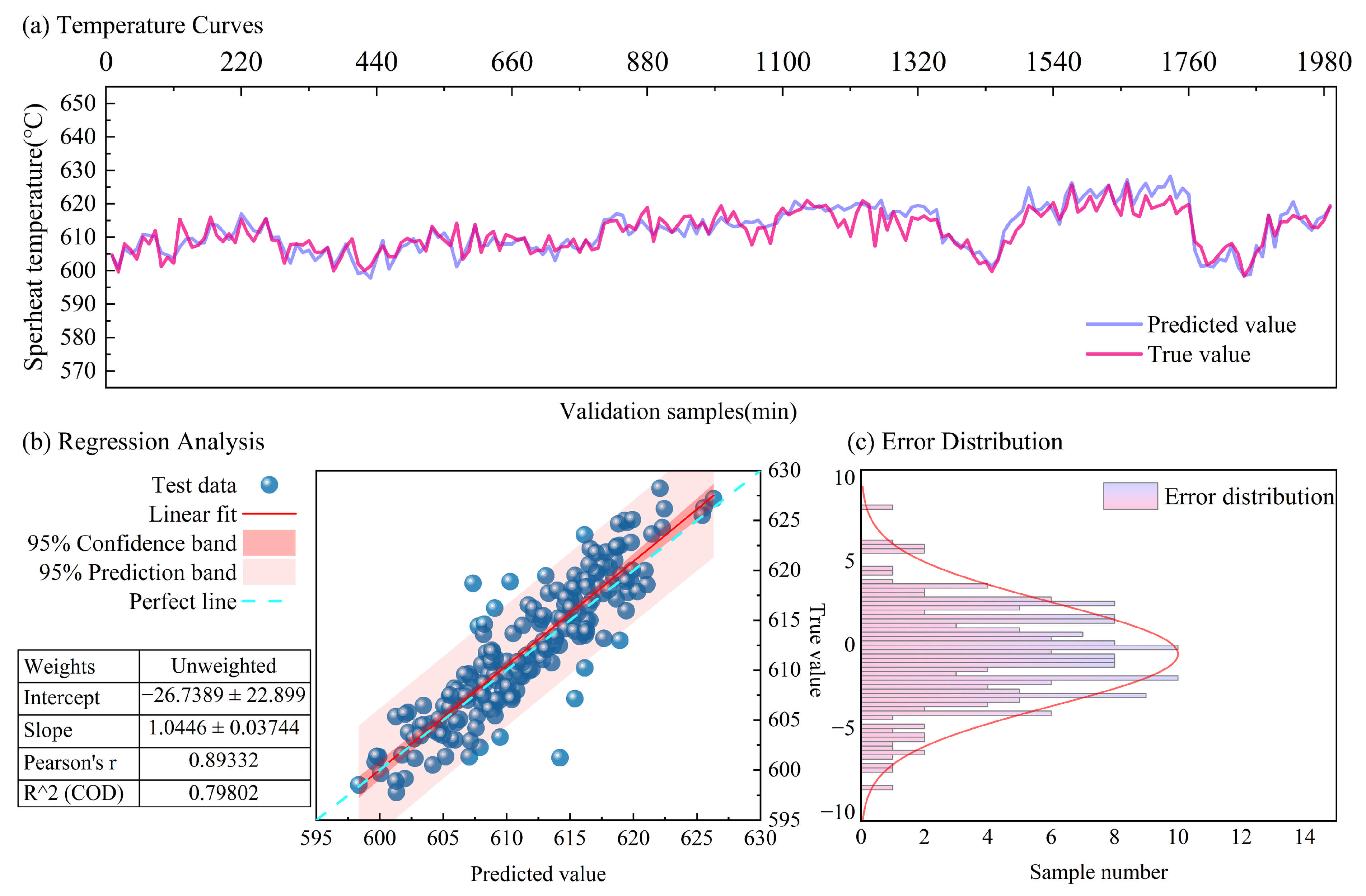
To further evaluate the industrial applicability of the proposed KAN model, a case study was conducted focusing on Measurement Point No. 2 of the high-temperature superheater wall, as introduced in Section 4.3. Figure 11 presents the single-step prediction performance of the KAN model. As shown in Figure 11a, the predicted and actual temperature curves exhibit strong alignment across the observed time window. Figure 11b illustrates the regression analysis results, where the fitted line has a slope of 1.0446 and an intercept of −26.7389, with a Pearson correlation coefficient of 0.893 and an R2 value of 0.798, indicating a high level of linear consistency between predicted and measured values. In addition, Figure 11c shows that the prediction errors are approximately normally distributed, with most errors falling within ±5 °C, confirming the robustness and generalization capability of the model under real operating noise and variability.
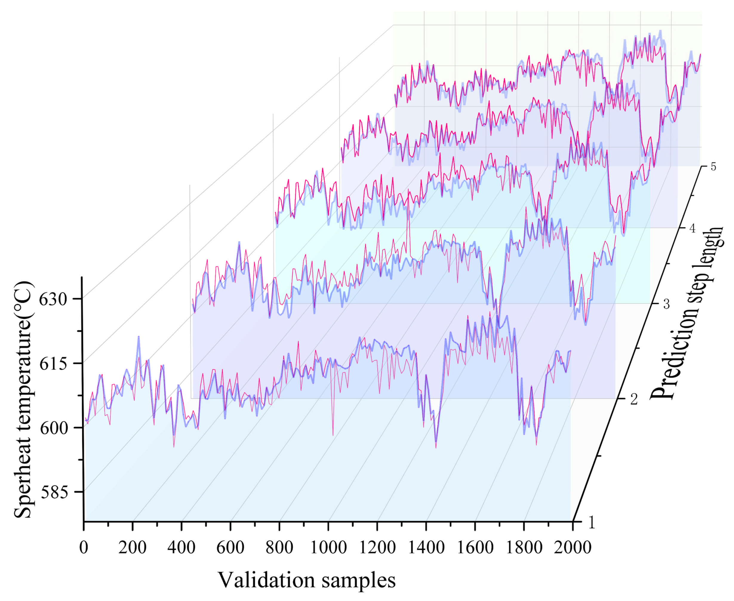
In addition to single-step prediction, a multi-step forecasting experiment was conducted to simulate short-term real-time prediction scenarios. As illustrated in Figure 12, the KAN model successfully tracks the future temperature evolution over a five-minute horizon and aligns well with the actual thermal response observed at Measurement Point No. 2. The performance metrics indicate that the model maintains consistent accuracy across multiple steps, with the average MAE, MAPE, RMSE, and R2 being 2.48 °C, 0.405, 3.33 °C, and 0.767, respectively. Notably, the model achieves its highest R2 of 0.82 at the fourth time step, while the lowest R2 of 0.70 occurs at the third step, reflecting slight fluctuations due to dynamic operation and input noise. Despite this, the model remains robust in capturing the overall temporal trend. This forecasting capacity is particularly relevant in light of the approximately 5 min delay typically observed between spray flow adjustments and wall temperature responses. The results suggest that the KAN model not only provides accurate instantaneous predictions but also supports proactive thermal regulation strategies by enabling the operator to anticipate temperature deviations in advance. Moreover, the KAN model enables advance prediction of wall temperature up to five minutes ahead, with fast inference performed at one-minute intervals. At each time step, the model forecasts the wall temperature five minutes into the future, in the subsequent cycle, it predicts four minutes ahead, and so on. Through this rolling prediction method, the model ensures continuous monitoring and provides actionable foresight, offering operators consistent and reliable support for decision-making.

4.3.3. Discussions

The experimental results directly address the limitations identified in previous studies. First, compared with conventional MLP-based models, the KAN framework demonstrates higher accuracy and lower variance under fluctuating operating conditions, and shows certain advantages in inference efficiency, thereby partially alleviating the issues of computational cost and stability that existed in earlier approaches. Second, unlike some models whose prediction accuracy rapidly deteriorates as the forecasting horizon increases, the proposed KAN maintains relatively stable performance in multi-step forecasting, indicating its reliability and applicability in short-term predictive tasks. Moreover, the model was validated across a wide load range of 300–975 MW under real operating noise, and the results confirm its strong robustness. This not only overcomes the limitation of many prior studies that validated models only under restricted experimental settings, but also provides evidence supporting its potential deployment across diverse operating conditions and unit types. In addition, this study systematically integrates feature selection, temporal dynamics modeling, and automated optimization into a unified framework, underscoring its deployability and practical value in industrial environments. It should be noted, however, that research on the KAN model is still at an exploratory stage, and compared with the more mature MLP architecture, it lacks long-term validation in large-scale industrial applications. Future work could further investigate the generalizability of KAN across different units and operating conditions, and explore its potential role in real-time optimization and control.

5. Conclusions

This study proposed a high-precision soft-sensing framework for predicting boiler high-temperature superheater wall temperatures, centered on a Kolmogorov–Arnold Network (KAN) optimized by the Polar Lights Optimization (PLO) algorithm. The framework integrates Random Forest–based feature selection, sliding-window temporal modeling, and automated hyperparameter tuning, systematically combining data preprocessing, feature extraction, model training, and validation into a unified pipeline.
Validation was conducted using 10,000 samples collected from a 1000 MW ultra-supercritical variable-pressure once-through boiler, with results showing that the proposed method consistently outperformed conventional multilayer perceptron (MLP) baselines. In single-step prediction, the PLO-KAN model achieved a Pearson correlation coefficient of 0.893 and an R2 of 0.798, with most errors distributed within ±5 °C. In multi-step forecasting, the model maintained stable performance within a five-minute prediction horizon, with average MAE, MAPE, RMSE, and R2 values of 2.48 °C, 0.405, 3.33 °C, and 0.767, respectively. These results demonstrate that the PLO-KAN framework delivers superior accuracy, robustness, and predictive consistency under dynamic thermal conditions, effectively addressing prior shortcomings such as high computational cost, instability, long-horizon degradation, and limited validation under real operating environments.
At the same time, the interpretability of KAN enhances the model’s credibility in industrial applications. Moreover, the model is capable of anticipating the delayed thermal response of boilers, enabling continuous monitoring and reliable short-term predictive foresight, thereby providing important engineering value for proactive thermal regulation, operational safety, and equipment lifespan extension.
Future research may further investigate the generalizability of the proposed framework across different units, its integration with advanced control strategies, and comparative studies with other deep learning architectures, in order to further improve interpretability, scalability, and industrial applicability.

Author Contributions

Conceptualization, Z.H. and X.P.; methodology, Z.H.; software, Z.H.; validation, Z.H., G.Y. (Guangmin Yang) and Y.W.; formal analysis, Z.W.; investigation, S.X.; resources, G.Y. (Ge Yin); data curation, J.G. and X.T.; writing—original draft preparation, Z.H.; writing—review and editing, Z.H. and X.P.; visualization, G.Y. (Guangmin Yang) and Y.W.; supervision, X.P.; project administration, C.H. and G.Y. (Ge Yin); funding acquisition, X.P. All authors have read and agreed to the published version of the manuscript.

Funding

This research was funded by the Open Project Program of the Xinjiang Key Laboratory of High Value Green Utilization of Low-rank Coal [grant number XJDX2314-YB202405], the National Natural Science Foundation of China (NSFC) [grant number 52574291], and the Basic Research Program of Xuzhou [grant number KC23050].

Data Availability Statement

The raw data supporting the conclusions of this article will be made available by the authors upon request.

Acknowledgments

The authors acknowledge the engineers of Huaneng Yingkou Thermal Power Plant and China Resources (Xuzhou) Electric Power Co., Ltd.

Conflicts of Interest

Author Shiming Xu was employed by the company Huaneng Yingkou Thermal Power Co., Ltd. Author Ge Yin was employed by the company China Energy Science and Technology Research Institute Co., Ltd. The remaining authors declare that the research was conducted in the absence of any commercial or financial relationships that could be construed as a potential conflict of interest.

References

  1. Kumar, S.; Tadge, P.; Mondal, A.; Hussain, N.; Ray, S.; Saha, A. Boiler tube failures in thermal power plant: Two case studies. Mater. Today Proc. 2022, 66, 3847–3852. [Google Scholar] [CrossRef]
  2. Yin, L.F.; Xie, J.X. Multi-feature-scale fusion temporal convolution networks for metal temperature forecasting of ultra-supercritical coal-fired power plant reheater tubes. Energy 2022, 238, 121657. [Google Scholar] [CrossRef]
  3. Yan, J.W.; Liu, X.; Huang, S.Y.; Yue, L.; Li, C.; Li, X.Y.; Wei, J.; Fu, J.; Li, W.J.; Wang, H.Y. Coupled model for prediction of water wall tube temperature of supercritical boiler. Therm. Power Gener. 2022, 51, 100–108. [Google Scholar] [CrossRef]
  4. Zhu, B.W.; Si, F.Q.; Dong, Y.S. Study on Tube Metal Temperature Distribution Characteristics of Final Superheater of Coal-Fired Boiler Based on CFD. Boil. Technol. 2024, 55, 13–20. [Google Scholar] [CrossRef]
  5. Wang, T.; Zhou, T.; Lu, J.; Wu, Y.; Zhang, T.; Ma, Y. Numerical simulation research on heat transfer characteristics of platen superheater of 660 MW coal-fired boiler. Meitan Xuebao/J. China Coal Soc. 2022, 47, 3860–3869. [Google Scholar] [CrossRef]
  6. Yu, Y.X.; Liao, H.K.; Wu, Y.L.; Zhong, W. Study on Tube Wall Temperature of Power Plant Boilers Based on Coupled Thermal Hydraulic Analysis. J. Chin. Soc. Power Eng. 2015, 35, 1–7. [Google Scholar] [CrossRef]
  7. Yu, C.; Si, F.Q.; Li, M.; Wu, H.L. Study on Overtemperature of Boiler Steam Tube base on Coupling Model of Combustion and Hydrodynamic. J. Eng. Therm. Energy Power 2021, 36, 92–98. [Google Scholar] [CrossRef]
  8. Jin, D.H.; Liu, X.; Zhang, X.Y.; Shen, Y.; Wang, T.; Li, C.; Li, X.Y.; Wei, J.; Fu, J.; Wang, H.Y. A Coupled Model for Predicting the Tube Temperature of Platen Superheater of Coal-fired Boiler. Proc. CSEE 2022, 42, 8951–8961. [Google Scholar] [CrossRef]
  9. Madejski, P.; Taler, D.; Taler, J. Thermal and flow calculations of platen superheater in large scale CFB boiler. Energy 2022, 258, 124841. [Google Scholar] [CrossRef]
  10. Cui, Z.P.; Xu, J.; Liu, W.H.; Zhao, G.J.; Ma, S.X. Data-driven modeling-based digital twin of supercritical coal-fired boiler for metal temperature anomaly detection. Energy 2023, 278, 127959. [Google Scholar] [CrossRef]
  11. Cao, Y.Y.; Mao, D.J.; Chen, S.Q. Boiler Heating Surface Wall Temperature Prediction based on TCN-Attention-BiGRU. Comput. Simul. 2025, 42, 91–98. Available online: https://link.cnki.net/urlid/11.3724.tp.20240328.1028.008 (accessed on 1 September 2025).
  12. Lu, B.; Liu, X.; Gao, L.; Zhao, X.L. Prediction model of boiler platen superheater tube wall temperature based on NARX neural network. Therm. Power Gener. 2019, 48, 35–40. [Google Scholar] [CrossRef]
  13. Laubscher, R. Time-series forecasting of coal-fired power plant reheater metal temperatures using encoder-decoder recurrent neural networks. Energy 2019, 189, 116187. [Google Scholar] [CrossRef]
  14. Wei, X.B.; Cui, Z.P.; Xu, J.; Ma, S.X. Data-driven method for predicting the wall temperature of heating surface of supercritical boilers. Therm. Power Gener. 2023, 52, 106–112. [Google Scholar] [CrossRef]
  15. Fan, Y.C.; Zhou, Y.Q.; Wei, C.; Liu, X.; Wang, H.Y. Data-driven Modeling for Over-temperature Prediction of Platen Superheater in Coal-fired Boiler. Proc. CSEE 2025, 1–11. [Google Scholar] [CrossRef]
  16. Yan, X.C.; Cao, H.; Hua, Y.P. Prediction on tube wall temperatures of boiler heating surfaces based on artificial intelligence. Integr. Intell. Energy 2022, 44, 58–62. [Google Scholar] [CrossRef]
  17. Sha, X.; Huang, Q.; Liu, G.Q.; Li, S.Q. Time Series Analysis of Monitored Heating Surface Wall Temperature of Coal-Fired Boiler. J. Combust. Sci. Technol. 2021, 27, 475–481. [Google Scholar] [CrossRef]
  18. Mcculloch, W.S.; Pitts, W. A Logical Calculus of the Ideas Immanent in Nervous Activity. Bull. Math. Biophys. 1943, 5, 115–133. [Google Scholar] [CrossRef]
  19. Rosenblatt, F. The perceptron: A probabilistic model for information storage and organization in the brain. Psychol. Rev. 1958, 65, 386–408. [Google Scholar] [CrossRef]
  20. Cybenko, G. Approximation by superpositions of a sigmoidal function. Math. Control. Signals Syst. 1989, 2, 303–314. [Google Scholar] [CrossRef]
  21. Hornik, K.; Stinchcombe, M.; White, H. Multilayer feedforward networks are universal approximators. Neural Netw. 1989, 2, 359–366. [Google Scholar] [CrossRef]
  22. Rumelhart, D.E.; Hinton, G.E.; Williams, R.J. Learning Representations by Back Propagating Errors. Nature 1986, 323, 533–536. [Google Scholar] [CrossRef]
  23. Krizhevsky, A.; Sutskever, I.; Hinton, G. ImageNet Classification with Deep Convolutional Neural Networks. Comput. Sci. 2014, 60, 84–90. [Google Scholar] [CrossRef]
  24. Simonyan, K.; Zisserman, A. Very Deep Convolutional Networks for Large-Scale Image Recognition. arXiv 2014, arXiv:1409.1556. [Google Scholar] [CrossRef]
  25. He, K.; Zhang, X.; Ren, S.; Sun, J. Deep Residual Learning for Image Recognition. In Proceedings of the 2016 IEEE Conference on Computer Vision and Pattern Recognition (CVPR), Las Vegas, NV, USA, 27–30 June 2016; pp. 770–778. [Google Scholar] [CrossRef]
  26. Wang, Z.; Xue, W.Y.; Li, K.Y.; Tang, Z.H.; Liu, Y.; Zhang, F.; Cao, S.X.; Peng, X.Y.; Wu, E.Q.; Zhou, H.C. Dynamic combustion optimization of a pulverized coal boiler considering the wall temperature constraints: A deep reinforcement learning-based framework. Appl. Therm. Eng. 2025, 259, 124923. [Google Scholar] [CrossRef]
  27. Chen, W.H.; Zhai, C.H.; Wang, X.; Li, J.; Lv, P.B.; Liu, C. GCN- and GRU-Based Intelligent Model for Temperature Prediction of Local Heating Surfaces. IEEE Trans. Ind. Inform. 2023, 19, 5517–5529. [Google Scholar] [CrossRef]
  28. Liu, Z.; Wang, Y.; Vaidya, S.; Ruehle, F.; Halverson, J.; Soljacic, M.; Hou, T.Y.; Tegmark, M. KAN: Kolmogorov-Arnold Networks. arXiv 2025, arXiv:2404.19756. [Google Scholar] [CrossRef]
  29. Yuan, C.; Zhao, D.; Heidari, A.A.; Liu, L.; Chen, Y.; Chen, H.L. Polar lights optimizer: Algorithm and applications in image segmentation and feature selection. Neurocomputing 2024, 607, 128427. [Google Scholar] [CrossRef]
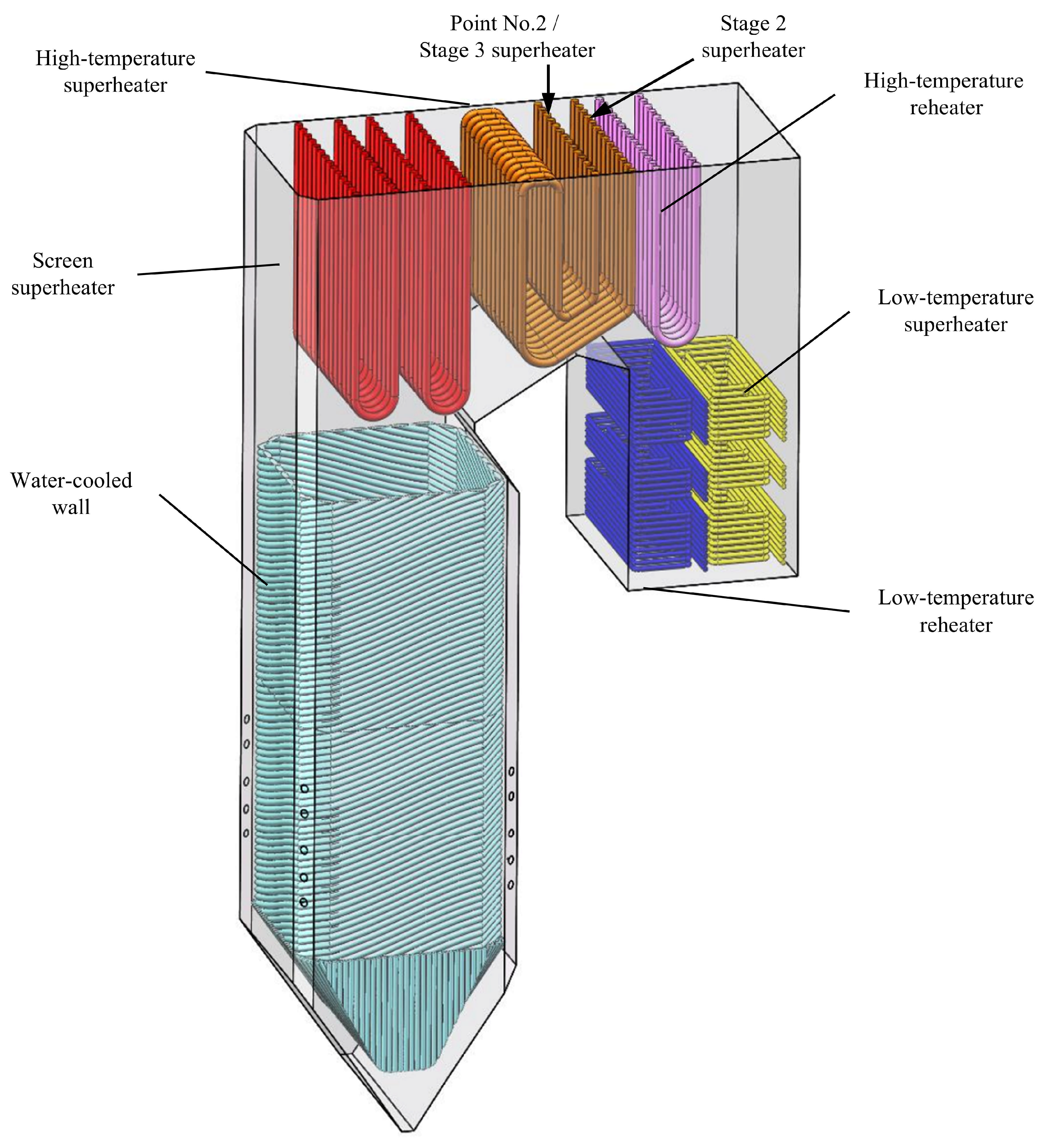
Figure 1. Schematic of main heating surfaces in the boiler.
Processes 13 03741 g001
Figure 2. Metal temperature response curve of Tube No. 2 on the high-temperature superheater wall.
Processes 13 03741 g002
Figure 3. Feature importance analysis of factors affecting superheater wall temperature.
Processes 13 03741 g003
Figure 4. Sliding Window Dataset Construction Diagram.
Processes 13 03741 g004
Figure 5. Schematic diagram of the Kolmogorov–Arnold Network (KAN) model.
Processes 13 03741 g005
Figure 6. Flowchart of the Polar Lights Optimization (PLO) algorithm.
Processes 13 03741 g006
Figure 7. Flowchart of the KAN model for PLO.
Processes 13 03741 g007
Figure 8. Research logic diagram.
Processes 13 03741 g008
Figure 9. Radar plots comparing performance metrics of KAN architectures with varying depths and widths.
Processes 13 03741 g009
Figure 10. Comparison of prediction errors between KAN and MLP models across load intervals.
Processes 13 03741 g010
Figure 11. Single-step prediction performance of the KAN model.
Processes 13 03741 g011
Figure 12. Multi-step prediction performance of the KAN model.
Processes 13 03741 g012
Table 1. Pseudo-code for the window sliding process.
StepsSliding Window (X, T, S):
1Initialize the set of subsequences
2Window list = Empty list
3Calculate the number of subsequences
4P = (LT)/S + 1
5Sliding window to extract subsequences
6Do this for i from 0 to (LT) per stride S:
7Extract the segment in the current window
8subsequences = X[i : i + T, :]
9list add(subsequences)
10Return all subsequences
11Return list
Table 2. Top 30 optimal hyperparameter configurations of the KAN model optimized by PLO.
No.Particle IDLearning RateWeight DecayMSELoss
11480.010.000123.6846
2750.0522540.00158.0932
3250.10.0000161.7773
4320.0455720.00164.2408
530.0416830.00095466.2496
6330.0509210.00020466.7475
7310.0933180.00059768.8121
8290.0299490.0000167.3473
940.0267700.00068467.9020
1010.0256030.00019368.2937
111250.10.00169.0940
121380.10.00169.8976
13280.0390750.00071674.3549
14830.0331890.00173.3565
15170.0235910.0006973.2457
16260.0287860.00173.6511
17500.0517360.00174.5700
18440.0144100.00174.0408
19410.0811730.00174.4267
20100.0856600.0000173.5209
211460.0416800.00176.8735
22220.0152760.00096776.4326
23180.0652410.00012376.6444
24450.0598520.0000177.7496
25770.0360080.00178.8363
26150.0657480.00027379.0833
27370.0461560.00179.5514
28300.0386320.00044379.6732
2950.0871690.00049278.5241
30200.0861540.0000182.9460
Disclaimer/Publisher’s Note: The statements, opinions and data contained in all publications are solely those of the individual author(s) and contributor(s) and not of MDPI and/or the editor(s). MDPI and/or the editor(s) disclaim responsibility for any injury to people or property resulting from any ideas, methods, instructions or products referred to in the content.