Improvement of Energy Performance of Glass Furnaces Using Modelling and Optimization Techniques

Abstract

Glass furnaces are a key component of the energy-intensive glass industry. Therefore, optimization of their energy performance is crucial for both economic and environmental sustainability. This study focused on optimizing the performance of an electric-boosted natural gas glass furnace. For this purpose, firstly, raw operational data were collected from a glass furnace. Next, reconciled data were obtained via a modelling process, data reconciliation, and gross error detection to establish a reliable dataset. Two linear regression models were developed and tested using both raw and reconciled data and compared with each other. The constrained optimization problem was constructed using a linear regression model and other process constraints and solved via the interior-point method to minimize specific energy consumption. The findings indicate that the reconciled data-based linear regression model yielded more reliable results. The specific energy consumption can be reduced to a minimum of 3660.088 kJ/kg-glass under an optimal setpoint for raw material, cullet, water, raw material temperature, electric boosting, and fuel. Furthermore, the analysis reveals that energy performance is enhanced with increased glass production and greater utilization of electric boosting. These results emphasize that the integrated statistical modelling approach provides valuable and actionable insights for energy performance improvements in the glass industry.

1. Introduction

The glass production sector is considered energy-intensive due to its high operating temperatures and the requirement for continuous production. Within this sector, glass furnaces are the most energy-demanding components and serve as the core of the manufacturing process [1,2,3]. These furnaces account for a significant portion of the total energy consumption in the industry (ranging from 70% to 90%). Increasing energy costs and high energy consumption have encouraged many industries around the world to use more efficient and optimized energy systems [4,5]. Moreover, increasing environmental degradation and commitments to reduce greenhouse gas emissions have made energy system optimization necessary [6]. Therefore, enhancing the energy performance of glass furnaces is critical not only for economic efficiency but also for environmental sustainability.

Traditionally, furnace performance has been improved through experimental observations, physical modelling, and engineering experience. However, these traditional methods often fail to produce sufficient results due to the variability and complexity of glass production processes such as variations in substance flow rates, cullet ratios, and air leaks. This situation highlights a critical need for data-driven approaches that can effectively process and interpret the vast datasets generated during production.

In recent years, statistical methods such as data-driven approaches have become an important tool for energy performance analysis [7]. In this context, techniques like stepwise linear regression can clearly identify relationships between process parameters and energy consumption, enabling accurate prediction and optimization of furnace performance. Ultimately, by combining these statistical models with optimization algorithms, it is possible to determine suitable operating conditions that ensure minimum energy consumption.

Improving the energy performance of glass furnaces has long been a critical topic for research. Traditional methods like mass and energy balance analysis [8] and physical process simulations [9] are widely used due to their high accuracy, and these techniques are based on fundamental physical principles. However, these methods have limitations in industrial applications, especially under dynamic process conditions such as variations in raw material flow rates, cullet ratios, and air leaks. These factors often render static physical models insufficient to reflect actual system behavior. Energy efficiency optimization is vital for reducing energy consumption, improving operational performance, and minimizing environmental impact. Strategies involving the influence of operational variables and the integration of advanced technologies into furnace design have led to significant progress toward more sustainable and cost-effective production processes.

The literature covers a broad range of topics concerning energy systems in glass production, including physical limits [10,11], the effect of changing electrode positions [12], and the use of solar energy in the melting process [13]. Other noteworthy studies include monitoring and control of glass furnaces with smart measurement methods [14], the effect of regenerator on energy performance [15], the effect of insulation of glass furnaces on energy performance [16], and the development of oxy-combustion systems instead of traditional combustion [11]. Energy systems encompass the technical and economic components used to convert energy from sources like natural gas, coal, or solar power [17]. Detailed comparisons of the performance of glass furnaces in general terms were first carried out by Beerkens et al. [18] and Sardeshpande et al. [1].

Performance analysis relies heavily on accurate data collection. In glass furnaces, high temperatures pose significant challenges to measurement. Measurements are usually made to determine mass flow rate, temperature, and pressure. Moreover, due to technical limitations and economic considerations, it is not possible to measure all variables in many systems [19]. In addition, each physical measurement may contain uncertainties such as random errors and systematic errors [20]. Many studies have been conducted to reduce these measurement uncertainties. For example, Zhou et al. [21] investigated the effect of measurement uncertainty of operating conditions on performance evaluation parameters in thermodynamic systems.

The process model of glass furnaces can be established both on a physical basis (thermodynamic laws, mass-energy balance) and on an empirical or statistical basis. Physical models are based on basic sciences such as thermodynamic laws, heat transfer, combustion kinetics, and fluid dynamics, while empirical or statistical models are based on the relationships between input–output variables, using real business data. Studies on the physical modelling of glass furnaces from the past to the present have been reviewed by Sardeshpande et al. [1], Sardeshpande et al. [2], Raič et al. [22], and Kodak et al. [8]. Yet, such models can provide valuable insights if the data quality and variable selection are robust.

Given the complexity of furnace operations, advanced data processing techniques like data reconciliation and gross error detection are essential for ensuring measurement accuracy [23]. These methods not only improve data reliability but also allow for the estimation of unmeasured variables. Recent studies have shown that the importance of optimization techniques based on data consensus in industrial processes has been increasing [24]. Technical advances in error detection, reconciliation, and efficiency analysis have enabled researchers to identify and correct data inconsistencies, resulting in better-quality analysis of energy efficiency. For example, in the study conducted by Adhi and Saputro [25], the importance of data reconciliation and gross error detection methods in industrial processes was emphasized, highlighting their importance in process efficiency analysis, process status monitoring, and operational optimization processes. With these methods, the accuracy and reliability of the information used in the evaluation of energy efficiency are slightly increased by contributing to the detection and regulation of errors in process data.

For example, Yuan et al. [26] used Bayesian methods for simultaneous gross error detection and data reconciliation and showed that the use of these methods increased the data accuracy and enhanced the ability to detect errors. Dumont et al. [27] conducted an analysis of cooling and power cycles of positive energy buildings using data reconciliation techniques. The innovative idea of using simulation techniques in processes such as optimizing the repositioning of electrodes in glass furnaces demonstrates the glass industry’s commitment to using advanced technologies to increase the energy efficiency of glass furnaces in industrial processes [12]. In addition, an issue that is currently relevant is the inclusion of electric-boosted units in glass furnaces to meet the challenges of increasing glass melting quality, energy efficiency, and production capacity without major changes in glass furnaces [28,29].

Statistical modeling methods are among the alternatives that can provide estimations of fuel consumption in energy systems. These are among the preferred methods in energy systems research in terms of understanding the relationships between variables more clearly, transparency of the model, and ease of application, especially with regard to linear regression analysis. Thanks to regression analysis, the key variables affecting energy consumption can be identified, energy systems can be modelled numerically, and the operation and behavior of processes can be predicted. There are many statistical studies in the literature. For example, Ma et al. [30] applied the use of machine learning algorithms to increase energy efficiency. Fialko et al. [31] used exergy analysis and statistical methods to optimize the geometric parameters of a glass furnace and improve energy efficiency. Using these models and optimization techniques, suitable operating conditions can be determined to enhance systems’ energy performance.

Numerous studies have focused on optimizing the energy performance of glass furnaces. Studies such as the optimization of process parameters [32] and improving energy performance [31] have attracted attention. For example, Reddy and P [33] measured some parts of energy systems using wireless sensors and used advanced optimization techniques such as ant colony optimization and firefly swarm optimization to optimize the energy efficiency of systems. Basso et al. [34] increased the energy efficiency of the glass furnace in the case study by optimizing operational parameters such as burner settings in oxygen-gas fired glass furnaces to increase the overall efficiency. Li [35] investigated the optimization of the residence time of the raw material in the glass furnace to increase the energy performance and carried out a computer simulation.

When the above studies are examined, a significant research gap still exists in the literature regarding the optimization of the energy performance of glass furnaces. A more efficient glass furnace can be achieved through the use of advanced data collection techniques, detailed process modelling, data reconciliation, linear regression models, and optimization algorithms. By combining these approaches, the challenges associated with increasing the energy performance of glass furnaces can be substantially mitigated. As a result, the effort to enhance energy efficiency in glass furnaces through data reconciliation and optimization methods represents a crucial step toward the sustainability of the glass industry.

The main contribution of this study is to reveal the basic process variables affecting energy consumption, through a regression model developed using the operational data obtained from a real electric-boosted natural gas furnace, and to determine the most appropriate operating parameters to increase the energy performance of this glass furnace by using these models. In this way, data-driven modeling can be performed and optimization can be conducted based on this model. In addition, this study makes a unique contribution to the literature in terms of presenting an integrated approach in which statistical modeling and process optimization are used together.

This study aims to identify the basic process variables affecting energy consumption in an electric-boosted natural gas glass melting furnace, to model the relationships between these variables and energy consumption using the linear regression method, and to optimize these relationships to determine the ideal operating conditions that enhance the energy performance. This study is also a continuation of our previous work [8], where a robust data reconciliation technique was employed to generate reliable and consistent datasets. For this purpose, a process model of a glass furnace was created. Subsequently, reconciled data were obtained using the process model and data reconciliation methodology. Based on the raw data and reconciled, two stepwise linear regression models were developed, and optimization of energy performance was realized. Then, the reliability of these models and optimization results was compared with each other. Leaving some parameters constant, the combustion heat and specific energy consumption values were examined according to the raw material and cullet variables. As a result, the evaluation of energy performance with optimization methods provides valuable insights into improving operational performance and reducing energy consumption. Furthermore, sustainable production and reduction of environmental impacts can also be achieved through these methods.

2. Materials and Methods

2.1. Electric-Boosted Natural Gas Fired Glass Furnaces

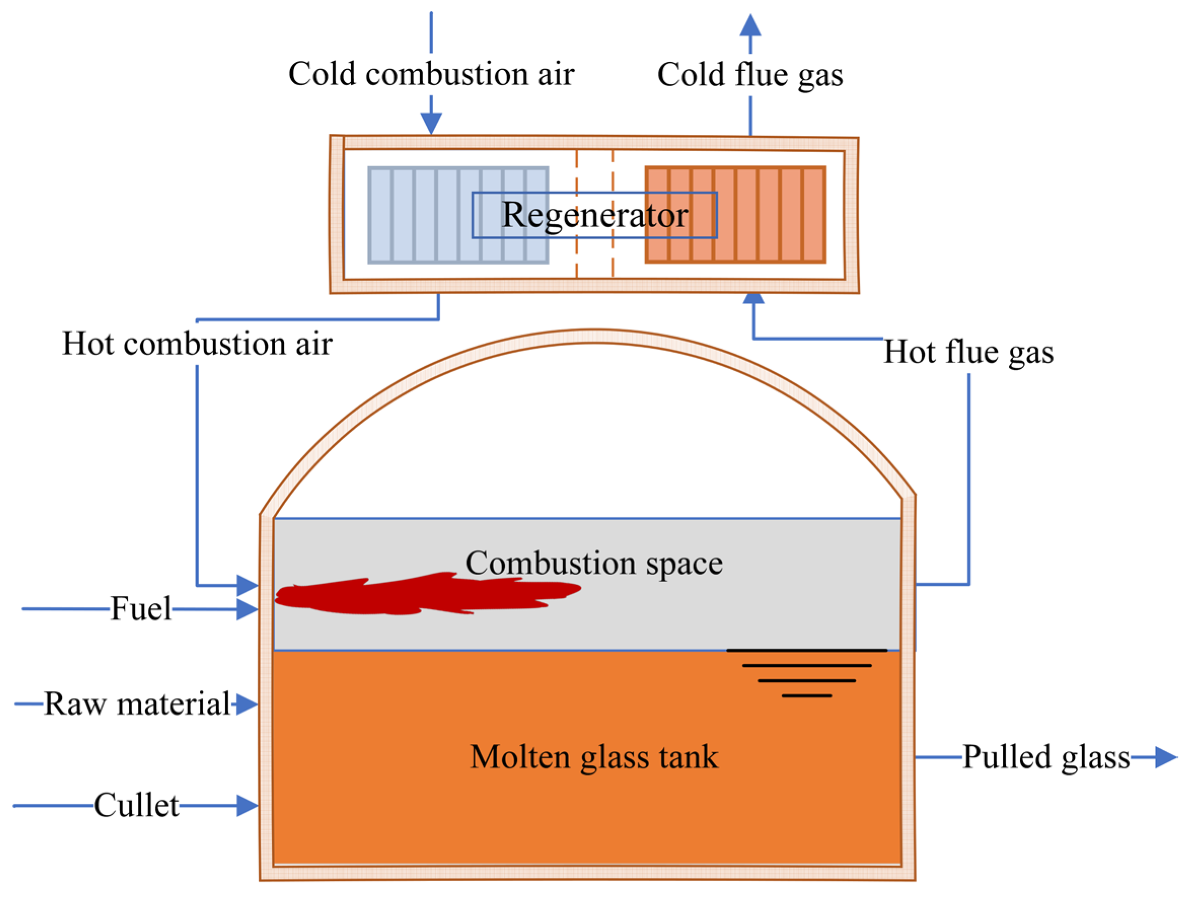
Today, electric-boosted natural gas glass furnaces are highly preferred in the glass industry due to reasons such as glass furnace product quality, production volume, high production speed, and low production cost [36]. Thanks to electric support, more homogeneous heat distribution in the glass melt and precise control of the temperature in the glass furnace are provided. Electric-boosted natural gas glass furnaces generally consist of three parts (Figure 1). These parts are the molten glass tank, combustion space, and regenerator [1].

The molten glass tank section is perhaps the most important part of the glass furnace. In the section, the raw material and cullet are melted, the purity of the glass is ensured, and the glass is made homogeneous. In addition, this part also contains electrodes. These electrodes provide direct energy to the glass melt, allowing it to heat more homogeneously. The combustion space provided heat for melting the raw material. In this part, heat is obtained by reacting natural gas and hot combustion air. The regenerator is used for heat transfer from flue gas to combustion air. In this way, regenerators make significant contributions to the increase in energy performance of glass furnaces.

2.2. Process Model

The process model of glass furnaces is obtained by mass and energy balance. The main objective of this process model is to analyze the thermodynamic and physical processes. Some assumptions are used to refine and idealize the glass furnace model. These assumptions include the following: the system operates under steady-state conditions; air, flue gas, and natural gas are assumed to be ideal gases; the inlet and outlet flow rates are considered constant; for wall heat transfer, the wall surface temperature is constant. A detailed process model of the glass furnace is provided in

Table A1. Process model of glass furnace [8].

Typology		Formulas
Mass balance	Molten glass tank	${\dot{m}}_{wt}+{\dot{m}}_{rm}+{\dot{m}}_{cul}={\dot{m}}_g+{\dot{m}}_{bg}$
	Combustion space	${\dot{m}}_{fu}+{\dot{m}}_{hca}+{\dot{m}}_{bg}+{\dot{m}}_{leak,brn}={\dot{m}}_{hflg}+{\dot{m}}_{leak,flg}$
	Regenerator	${\dot{m}}_{hflg}+{\dot{m}}_{leak,RDC}={\dot{m}}_{cflg} (Hot side)$ ${{\dot{m}}_{cca}=\dot{m}}_{hca} (Cold side)$
Atomic mass balance (For each atom)	Molten glass tank (Al, C, Ca, Co, Cr, Fe, H, K, Mg, Na, O, S, Si, and Ti)	$$\begin{gathered} \mathbf{Al}\mathbf{:} 0.5293·w_{\mathrm{1,2}}·{\dot{m}}_{rm}+0.5293·w_{\mathrm{2,2}}·{\dot{m}}_{cul}- \\ 0.5293·w_{\mathrm{3,2}}·{\dot{m}}_g=0 \end{gathered}$$ $⋮$ $$\begin{gathered} \mathbf{Ti}: 0.5993·w_{\mathrm{1,4}}·{\dot{m}}_{rm}+0.5993·w_{\mathrm{2,4}}·{\dot{m}}_{cul}- \\ 0.5993·w_{\mathrm{3,4}}·{\dot{m}}_g=0 \end{gathered}$$
	Combustion space (C, H, N, O, and S)	$$\begin{gathered} \mathbf{C}\mathbf{:} 0.4288·w_{\mathrm{4,1}}·{\dot{m}}_{bg}+0.2729·w_{\mathrm{4,2}}·{\dot{m}}_{bg}+ \\ 0.7487·w_{\mathrm{5,1}}·{\dot{m}}_{fu}+0.7989·w_{\mathrm{5,2}}·{\dot{m}}_{fu}+0.8171· \\ {w}_{\mathrm{5,3}}·{\dot{m}}_{fu}-0.4288·w_{\mathrm{7,1}}·{\dot{m}}_{hflg}-0.2729·w_{\mathrm{7,2}}· \\ {\dot{m}}_{hflg}=0 \end{gathered}$$ $⋮$ $\mathbf{S}\mathbf{:} 0.5005·w_{\mathrm{4,5}}·{\dot{m}}_{bg}-0.5005·w_{\mathrm{7,7}}·{\dot{m}}_{hflg}=0$
	Regenerator (C, H, N, O, and S)	$$\begin{gathered} \mathbf{C}\mathbf{:} 0.4288·w_{\mathrm{7,1}}·{\dot{m}}_{hflg}+0.2729·w_{\mathrm{7,2}}·{\dot{m}}_{hflg}- \\ 0.4288·w_{\mathrm{9,1}}·{\dot{m}}_{cflg}-0.2729·w_{\mathrm{9,2}}·{\dot{m}}_{cflg}=0 \end{gathered}$$ $⋮$ $\mathbf{S}\mathbf{:} 0.5005·w_{\mathrm{7,7}}·{\dot{m}}_{hflg}-0.5005·w_{\mathrm{9,7}}·{\dot{m}}_{cflg}=0$
Normalization (for mass fractions)		$\begin{array}{l}{w}_{\mathrm{1,1}}+w_{\mathrm{1,2}}+w_{\mathrm{1,3}}+w_{\mathrm{1,4}}+w_{\mathrm{1,5}}+w_{\mathrm{1,6}}+ w_{\mathrm{1,7}}\\ +w_{\mathrm{1,8}}+ w_{\mathrm{1,9}}+w_{\mathrm{1,10}}+w_{\mathrm{1,11}}\\ +w_{\mathrm{1,12}}+w_{\mathrm{1,13}}+w_{\mathrm{1,14}}+w_{\mathrm{1,15}}\\ -1=0\end{array}$ $⋮$ $w_{\mathrm{13,1}}+w_{\mathrm{13,2}}-1=0$
Energy balance	Molten glass tank	$$\begin{gathered} {\dot{Q}}_{melt}+{\dot{W}}_{el}+{\dot{H}}_{wt}+{\dot{H}}_{rm}+{\dot{H}}_{cul} \\ ={\dot{H}}_g+{\dot{H}}_{bg}+∆H_{r,hofreac} \\ +{\dot{Q}}_{wall,MT} \end{gathered}$$
	Combustion space	$$\begin{gathered} {\dot{H}}_{fu}+{\dot{H}}_{hca}+{\dot{H}}_{bg}+{\dot{Q}}_{comb}+{\dot{H}}_{leak,brn} \\ ={\dot{H}}_{hflg}+{\dot{Q}}_{melt}+{\dot{H}}_{leak,flg} \\ +{\dot{Q}}_{wall,CS} \end{gathered}$$
	Regenerator	$$\begin{gathered} {\dot{H}}_{hflg}+{\dot{H}}_{leak,RDC} \\ ={\dot{H}}_{cflg}+{\dot{Q}}_{htbyrg} \\ +{\dot{Q}}_{wall,RDH} (Hot side) \end{gathered}$$ ${\dot{H}}_{cca}+{\dot{Q}}_{htbyrg}={\dot{H}}_{hca}+{\dot{Q}}_{wall,RDC}(Cold side)$
	Enthalpy (Ref. temp.: 273.15 K)	$$\begin{gathered} {\dot{H}}_i={\dot{m}}_i·\left(h_i-h_{i,273.15 K}^o\right) \\ ={\dot{m}}_i \\ ·\underset{T_{ref}}{\overset{T_{mat.}}{\int }}\left({\sum }_{j=1}^n{w}_{i,j}·c_{p,\left(i,j\right)}\left(T\right)\right)dT \end{gathered}$$
	Wall heat transfer	${\dot{Q}}_{wall,conv,i}=A_{wall,i}·h_i·\left(T_{wall,i}-T_{amb,i}\right)$ ${\dot{Q}}_{wall,rad,i}={\epsilon ·\sigma ·A}_{wall,i}·\left(T_{wall,i}^4-T_{amb,i}^4\right)$
Performance indicator	Energy efficiency	${\eta }_{GF}={\displaystyle \frac{{\dot{H}}_g}{{\sum {\dot{H}}_{sensible heat of inputs}+\dot{Q}}_{comb}+{\dot{W}}_{el}}}$
	Regenerator efficiency	${\eta }_{reg}={\displaystyle \frac{{\dot{H}}_{hca}-{\dot{H}}_{cca}}{{\dot{H}}_{hflg,sens}}}$
	Specific energy consumption	$SEC={\displaystyle \frac{{\dot{Q}}_{comb}+{\dot{W}}_{el}}{{\dot{m}}_g}}$

(Appendix A).

Mass and Energy Balance

Mass and energy analysis of glass furnaces is very important for the reliable and controlled execution of the glass production process. Mass balance assumes that the total incoming mass is equal to the total outgoing mass, given a steady-state condition. Mass balance helps to examine the balance between glass raw material, cullet, various additives, gaseous fluids, and molten glass. The mass balance analysis is examined in detail in the research article by [8]. Mass balance for the steady state is given in Equation (1):

$$\sum {\dot{m}}_{in}-\sum {\dot{m}}_{out}=0$$

(1)

where ${\dot{m}}_{in}$ and ${\dot{m}}_{out}$ are the inlet mass flow rate and outlet mass flow rate, respectively. Atomic mass balance assumes that the same atomic mass entering the system boundary is equal to the atomic mass exiting the system boundary. The atomic mass balance is given in Equation (2):

$$\sum _i^m\left({\sum }_{j=1}^n \underset{\begin{array}{c}Incidence\\ matrix\end{array}}{\underbrace{L_j·a_k·w_{i,j}}}\right)·{\dot{m}}_i=0$$

(2)

where $L$ is the sing (if the component $i$ enter node j $L_i=1$, if the component $i$ leaves node j $L_i=-1$, otherwise $L_i=0$), $a_k$ is the mass fraction of the atom in the molecule, and ${\dot{m}}_i$ is the mass flow rate.

Energy balance assumes that under the same steady-state conditions, the incoming energy is equal to the outgoing energy. It represents a balance between the energy entering and outcoming in the system boundaries. The energy balance for the steady-state is given in Equation (3):

$${\dot{Q}}_{in}+{\dot{W}}_{in}+\sum _{\begin{array}{c}i=1\\ in\end{array}}^n\dot{m_i}{h}_i-{\dot{Q}}_{out}-{\dot{W}}_{out}-\sum _{\begin{array}{c}j=1\\ out\end{array}}^n\dot{m_j}{h}_j=0$$

(3)

where ${\dot{Q}}_{in}$ and ${\dot{Q}}_{out}$ are heat entering the system and leaving the system, $m$ is the mass flow rate of each component, and $h$ is the specific enthalpy of each component.

2.3. Data Collection and Measurement

Data collection is usually carried out with sensors and measuring instruments. Measurements are usually obtained by direct observation, instrumentation, or specialized measurement techniques. Measurement in glass furnaces is usually performed using a combination of measuring instruments and laboratory tests. For mass flow rate measurements, automatic weighing systems with load cells, turbine flowmeters, orifice flowmeters, and mass flow meters are employed. To measure the temperatures of materials, thermocouples, thermal cameras/optic pyrometers, and suction pyrometers are used. For chemical composition analysis, laboratory techniques such as XRF/XRD analysis, gas chromatography, and oxygen analyzers are utilized [8].

Because of various physical limitations, these measurements are never perfect and inherently contain some degree of measurement error. Due to these challenges, data collection and measurement in glass furnaces can be extremely complex, and no data can be collected from some areas. Therefore, the accuracy and reliability of the measurement data and the analysis of unmeasured values via specific methods are of critical importance. In this context, data reconciliation and gross error detection methods can be effectively applied as solutions.

2.4. Nonlinear Data Reconciliation

Mass and energy balance analysis is typically performed using data reconciliation and gross error detection methods. This process enables the filtering of the measured data, estimation of unmeasured data, and quantitative analysis of key parameters such as energy consumption and energy performance.

Data reconciliation is a powerful analysis method in which reconciled and estimated values are obtained using mathematical models, error models, and measurement data [37]. This method is a methodology that minimizes both random and systematic error and ensures that the optimal solution is found under the physical and mathematical constraints. Thanks to this approach, a process model and measurement dataset that are initially inconsistent can be made consistent using reconciliation techniques. This method is widely used, especially in data analysis, energy systems, and industrial processes.

Nonlinear data reconciliation involves a system of nonlinear constraint equations. Therefore, reconciled estimated values must be obtained through numerical methods, rather than closed-form solutions. The formulation used for measured and reconciled variables is given by Equation (4):

$$y=x+ϵ$$

(4)

where $\mathrm{y}$ is the measured variable, $\mathrm{x}$ is the reconciled variable, and $\mathsf{ϵ}$ is the measurement error. A general formulation of a nonlinear data reconciliation problem is given in Equation (5a) and Equation (5b). The objective function $J$ is minimized, and the equality and inequality constraints are satisfied.

$$Minimize J=\sum _{i=1}^L{\left({\displaystyle \frac{y_i-x_i}{{\sigma }_i}}\right)}^2=(\mathit{y}-\mathit{x})\mathit{\Psi }(\mathit{y}-\mathit{x})$$

(5a)

$$\begin{array}{l}subject to:\\ {\phi }_k\left(x_i,u_j\right)=0\hspace{1em}k=1,\dots ,N\\ x_{min}<x_i<x_{max}\hspace{1em}i=1,\dots ,L\\ u_{min}<u_j<u_{max}\hspace{1em}j=1,\dots ,M\end{array}$$

(5b)

where $\mathrm{J}$ is the weighted least squares (WLS) objective function, y is the measurement variable, $x$ is the reconciled variable, $u$ is the unmeasured or estimated variable, $\sigma$ is the standard deviation of the measurements, and $\mathit{\Psi }$ is the covariance matrix of measured variables. ${\phi }_{\mathrm{k}}\left({\mathrm{x}}_{\mathrm{i}},{\mathrm{u}}_{\mathrm{j}}\right)$ presents a set of N linear and nonlinear physical constraints. This problem can be solved with a successive linearization algorithm [38], which is frequently used in data reconciliation problems. The equations required for implementing the successive linearization algorithm are provided in

Table 1. The formulas needed for the successive linearization algorithm [38].

Description	Formula	Equation
Error model	$y=x+ϵ,\hspace{1em}ϵ\sim N(0,{\sigma }^2)$	(6)
Linearized constraint model	$c_i=A_1{x}_i+A_2{u}_i-\phi \left(x_i,u_i\right)$	(7)
Jacobian matrices of measured and unmeasured variables	$A_1={\left.{\displaystyle \frac{\partial \phi \left(x,u\right)}{\partial x}}\right|}_{x=x^i}{A}_2={\left.{\displaystyle \frac{\partial \phi \left(x,u\right)}{\partial u}}\right|}_{u=u^i}$	(8)
Projection matrix and residual vector	$G_x=Q_{u2}^T{A}_1 and b=Q_{u2}^T{c}_i$	(9)
Reconciled variables	$x=y-\Psi G_x^T{\left(G_x\Psi G_x^T\right)}^{-1}(G_{x}y-b)$	(10)
Calculated (estimated) variables	$u_{ru}=R_{u1}^{-1}{Q}_{u1}^T{c}_i-R_{u1}^{-1}{Q}_{u1}^T{A}_{1}x$	(11)

.

Gross error detection identifies sensor failures, operator errors, or instantaneous deviations during the correction of measurement errors by identifying abnormal measurements and increasing system accuracy and reliability. In other words, if there is any error in the variable values of a process model (laboratory test data, sensor data, and data from measuring devices), gross error detection methods can mostly detect gross errors. Gross errors can be detected by global testing, nodal or constraint testing, or measurement testing [8].

2.5. Linear Regression Model

2.5.1. Data Supplement

For linear regression, two separate linear regression models were created using both raw and reconciled data. Raw data were obtained from factory measurement devices and experimental tests, while reconciled data were obtained using the data reconciliation methodology described and implemented in detail in our previous study [8]. Overall, using reconciled data instead of raw data increases the reliability and consistency of the model by eliminating potential errors in the raw data [38].

2.5.2. Methodology and Formulation

The linear regression model is a statistical technique used to model the relationship between a dependent variable and independent variables. Linear models are used to estimate the relationship between the dependent variable and the independent variables. The formulation of the linear regression model is presented below [39].

The basic linear regression model is given by Equation (12)

$$\underset{\begin{array}{c}Response\\ variables\end{array}}{\underbrace{\mathit{Y}}}=\underset{\begin{array}{c}Model\\ function\end{array}}{\underbrace{\mathit{f}\left(\mathit{\theta },\mathit{X}\right)}+}\underset{\begin{array}{c}Random\\ error\end{array}}{\underbrace{\mathit{\epsilon }}}$$

(12)

where $\mathit{Y}$ represents the response variables, $\mathit{f}\left(\mathit{\theta },\mathit{X}\right)$ is the model function, and $\mathit{\epsilon }$ is the random error. The model function depends on predictor variables $\mathbf{X}$ and parameters $\mathit{\theta }$. Each linear model term contains a constant term, linear terms, interaction terms (cross terms), quadratic terms, and error terms. The generalized form of this equation is given in Equation (13):

$${\mathit{y}}_{\mathit{i}}\left({\mathit{x}}_{\mathit{i}}\right)=\underset{constant}{\underbrace{c_0}}+\underset{Linear terms}{\underbrace{\sum _{i=1}^n{c}_i·{\mathit{x}}_{\mathit{i}}}}+\underset{\begin{array}{c}Interaction terms\\ (Cross terms)\end{array}}{\underbrace{\sum _{i,j\left(i\le j\right)}{c}_{i,j}·{\mathit{x}}_{\mathit{i}}·{\mathit{x}}_{\mathit{j}}}}+\underset{Quadratic terms}{\underbrace{\sum _{k=1}^n{c}_k·{\mathit{x}}_{\mathit{k}}^2}}+\underset{\begin{array}{c}Error\\ terms\end{array}}{\underbrace{{\mathit{\epsilon }}_{\mathit{i}}}}$$

(13)

The linear regression model consists of $n$ observation variables and $(m+1)$ parameters. This model can be simplified in matrix form, as shown in Equation (14):

$$\mathit{Y}={\left[\begin{array}{c}{Y}_1\\ Y_2\\ \dots \\ \dots \\ Y_n\end{array}\right]}_{nx1}, \mathit{X}={\left[\begin{array}{c}1\\ 1\\ \dots \\ \dots \\ 1\end{array}\begin{array}{c}{X}_{\mathrm{1,1}}\\ X_{\mathrm{1,2}}\\ \dots \\ \dots \\ X_{1,n}\end{array}\begin{array}{c}{X}_{\mathrm{2,1}}\\ X_{\mathrm{2,2}}\\ \dots \\ \dots \\ X_{2,n}\end{array}\begin{array}{c}\dots \\ \dots \\ \ddots \\ \dots \\ \dots \end{array} \begin{array}{c}\dots \\ \dots \\ \dots \\ \ddots \\ \dots \end{array}\begin{array}{c}{X}_{m,1}\\ X_{m,2}\\ \dots \\ \dots \\ X_{m,n}\end{array}\right]}_{nx\left(m+1\right)}, \mathit{\theta }={\left[\begin{array}{c}{\theta }_0\\ {\theta }_1\\ {\theta }_2\\ \dots \\ \dots \\ {\theta }_m\end{array}\right]}_{(m+1)x1},\mathit{\epsilon }={\left[\begin{array}{c}{\epsilon }_1\\ {\epsilon }_2\\ \dots \\ \dots \\ {\epsilon }_n\end{array}\right]}_{nx1}$$

(14)

In this matrix form, $\mathit{Y}$ is $n\times 1$ vector of observations, and X is an $n\times (m+1)$ matrix of known inputs, $\mathit{\theta }$ is $(m+1)\times 1$ vector of parameters, $\mathit{\epsilon }$ is an (n × 1) vector of errors. The linear regression model can be represented as the system of equations shown in Equation (15):

$$\mathit{Y}=\mathit{X}\mathit{\theta }+\mathit{\epsilon }$$

(15)

When these system equations $\mathit{Y}=\mathit{X}\mathit{\theta }$ are examined, it is understood that the system of equations is inconsistent. These inconsistent equations are transformed into a consistent system using the least squares method. The system can be expressed as the normal equations shown in Equation (16):

$${\mathit{X}}^{\mathit{T}}\mathit{Y}={\mathit{X}}^{\mathit{T}}\mathit{X}\mathit{\theta }$$

(16)

If ${\mathrm{d}\mathrm{e}\mathrm{t}(\mathbf{X}}^{\mathbf{T}}\mathbf{X})$ is not equal to zero, the normal equation has a unique solution (consistent): otherwise, it has either infinitely many solutions or no solution. The normal equations can be solved, and the parameters $\mathit{\theta }$ can be obtained by Equation (17):

$$\mathit{\theta }={\left({\mathit{X}}^{\mathit{T}}\mathit{X}\right)}^{-1}{\mathit{X}}^{\mathit{T}}\mathit{Y}$$

(17)

The fitted values (response variables) are given by Equation (18):

$$\widehat{\mathit{Y}}=\mathit{X}\mathit{\theta }$$

(18)

The sum of squared error ${\mathit{\epsilon }}^{\mathit{T}}\mathit{\epsilon }$ is given by Equation (19):

$${\mathit{\epsilon }}^{\mathit{T}}\mathit{\epsilon }={\left(\mathit{Y}-\mathit{X}\mathit{\theta }\right)}^{\mathit{T}}\left(\mathit{Y}-\mathit{X}\mathit{\theta }\right)$$

(19)

The coefficient of determination $R^2$ (R-squared) is a measure that provides information about the goodness of fit of a regression model. The $R^2$ value can be calculated by Equation (20):

$$R^2={\displaystyle \frac{{\mathit{\theta }}^{\mathit{T}}{\mathit{X}}^{\mathit{T}}\mathit{Y}-n·{\overline{Y}}^2}{{\mathit{Y}}^{\mathit{T}}\mathit{Y}-n·{\overline{Y}}^2}}$$

(20)

where n is the number of observations, and $\overline{Y}$ is the mean of all observations. The R-squared value ranges between 0 and 1. This value indicates how well the model is explained by the independent variables.

2.5.3. Model Selection and Stepwise Regression

Effective model selection is crucial for developing a robust linear regression model. The stepwise linear regression model is a method for analyzing linear regression by eliminating redundant independent variables. This method is applied to determine whether certain variables should be included in the model or not. To select the best regression equation, the stepwise linear regression method is applied using backward elimination algorithms. The backward elimination procedure is given below [39].

The backward elimination procedure is as follows:

• Compute a full linear regression model using all available independent variables.
• Calculate the partial p-value for every predictor variable.
• Identify the variable with the highest p-value, donated as p_max
• Compare p_max with a predefined significance threshold α (commonly corresponding to α = 0.05).
• Decision:
• If p_max > α, remove the variable associated with p_max. Then, return to Step 2 and recompute the regression model using the remaining variables.
• If p_max < α, stop the process and accept the current regression model as the optimal regression model.
• Program end.

2.6. Glass Furnace Performance Optimization

Performance for enhancing the energy efficiency of glass furnaces is carried out by solving a constrained optimization problem. An optimization problems usually consist of the objective function $f\left(x\right)$, equality constraints $h_i\left(x\right)$, inequality constraints $g_j\left(x\right)$, and upper $x_k^{upper}$ and lower $x_k^{lower}$ bounds. The general form of optimization problems is given in Equation (21), as follows:

$$\begin{gathered} \mathbf{Objective} \mathbf{function}: \underset{x}{\mathit{min}} f\left(x\right) \\ \mathbf{Constraints}: \\ {h}_i\left(x\right)=0,\hspace{1em}i=1,2,3,\dots , m \\ {g}_j\left(x\right)\le 0,\hspace{1em}j=1,2,3,\dots , n \\ \mathbf{Bounds}: x_k^{lower}\le x_k\le x_k^{upper} \end{gathered}$$

(21)

Each optimization algorithm aims to find the optimum solution of the objective function by considering equality and inequality constraints, and upper and lower bounds. To analyze and optimize the specific energy consumption of glass furnaces, the following are required: a predictor and response dataset, a linear regression model, and generally accepted optimization algorithms. In this study, specific energy consumption is selected as the objective function. Linear regression model and additional equations are used for equality constraints. Cullet rate and humidity are determined as inequality constraints.

The interior-point method was employed to solve this constrained optimization problem. This optimization solution method is particularly suitable for large-scale, nonlinear unconstrained optimization problems. The optimization problem was performed using MATLAB R2023b’s Optimization Toolbox to find an optimal set of operation variables to minimize the specific energy consumption of the glass furnace.

3. Results and Discussion

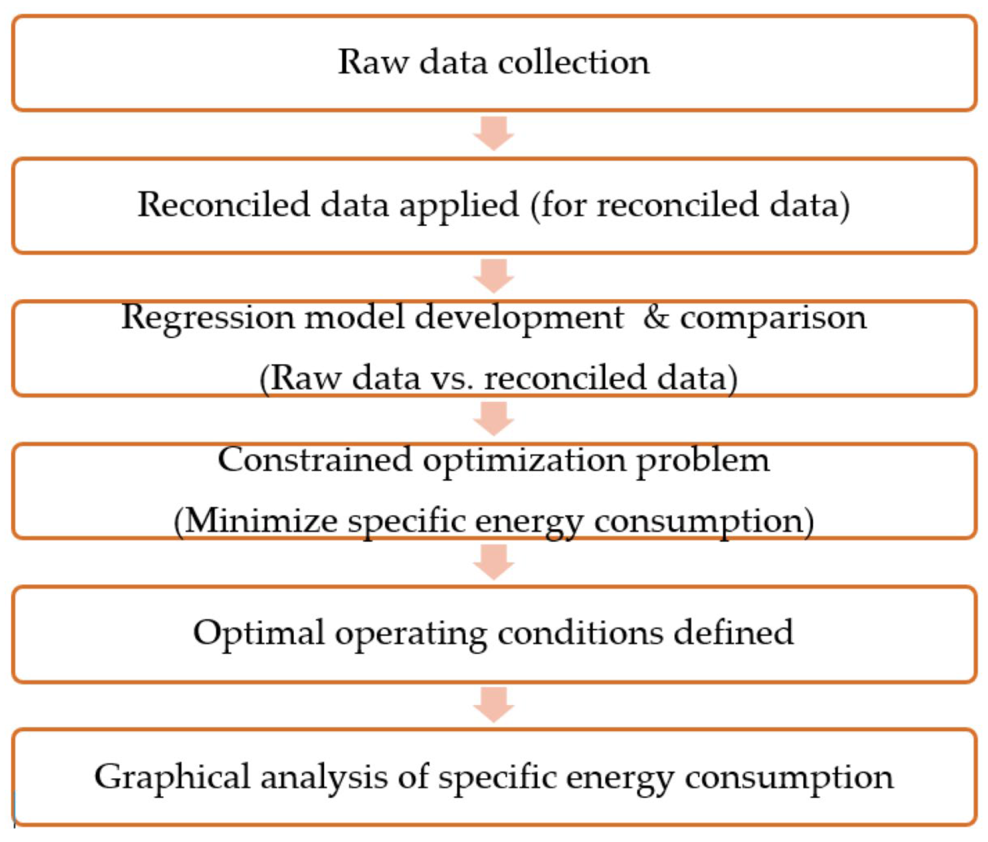
To optimize the energy performance of glass furnaces, a process model of a glass furnace was developed. Then, reconciled data were obtained through this process model and data reconciliation and gross error detection techniques. From these reconciled datasets, specific variables were selected as predictor and response variables for the linear regression model. Based on these variables and the dataset, the stepwise linear regression model was established. After these model parameters were determined, an optimization process was performed on this regression model. The required steps for the optimization process are illustrated in Figure 2.

3.1. Data Reconciliation and Performance Indicators Results

The process model of the glass furnace (including mass and energy balance) was created, and a data reconciliation methodology was applied using this process model and measurement data. Using the process model and data reconciliation methods, a reconciled dataset for 151 days was obtained. The reconciled dataset included variables such as mass flow rates, temperatures, mass fraction, electric boosting, furnace, and specific energy consumption. Descriptive statistics (mean, minimum, and maximum) of the raw and reconciled data are presented in

Table 2. Descriptive statistics (mean, minimum, and maximum) of the raw and reconciled process data.

Name	Raw Data		Reconciled Data
	Average	Min–Max Values	Average	Min–Max Values
Raw material	408.86 ton	318.08–479.86 ton	408.80 ton	318.03–479.50 ton
Cullet	79.37 ton	50.69–126.36 ton	79.38 ton	50.70–126.37 ton
Water	13.14 ton	6.91–16.93 ton	13.12 ton	6.90–16.90 ton
Raw material temperature	306.24 K	294.15–314.15 K	306.23 K	294.14–314.12 K
Electric boosting	42.74 GJ	0–157.24 GJ	42.75 GJ	0–157.25 GJ
Combustion heat	1717.27 GJ	1341.53–1949.41 GJ	1716.94 GJ	1341.79–1948.81 GJ
Specific energy consumption	$4197.52 {\displaystyle \frac{\mathrm{k}\mathrm{J}}{\mathrm{k}\mathrm{g} \mathrm{g}\mathrm{l}\mathrm{a}\mathrm{s}\mathrm{s}}}$	$3888.97\text{–}4652.57 {\displaystyle \frac{\mathrm{k}\mathrm{J}}{\mathrm{k}\mathrm{g} \mathrm{g}\mathrm{l}\mathrm{a}\mathrm{s}\mathrm{s}}}$	$4196.34 {\displaystyle \frac{\mathrm{k}\mathrm{J}}{\mathrm{k}\mathrm{g} \mathrm{g}\mathrm{l}\mathrm{a}\mathrm{s}\mathrm{s}}}$	$3888.41\text{–}4650.57 {\displaystyle \frac{\mathrm{k}\mathrm{J}}{\mathrm{k}\mathrm{g} \mathrm{g}\mathrm{l}\mathrm{a}\mathrm{s}\mathrm{s}}}$
Glass	420.09 ton	323.02–487.80 ton	420.13 ton	323.06–488.02 ton
Cullet/glass rate	18.80%	14.83–28.22%	18.80%	14.84–28.22%
Water/raw material rate (Humidity)	3.21%	2.06–3.73%	3.21%	2.06–3.72%

.

The most important performance indicator for glass furnaces is specific energy consumption. Here, the specific energy consumption ranged from 3880.87 to 4644.10 kJ/kg-glass. This variation was mainly due to daily fluctuations in raw material usage, glass production rates, utilization of electric boosting, and the mass flow rate of the cullet. As a result, the specific energy consumption exhibited considerable daily variability.

3.2. Statistical Analysis of Data Reconciliation Results

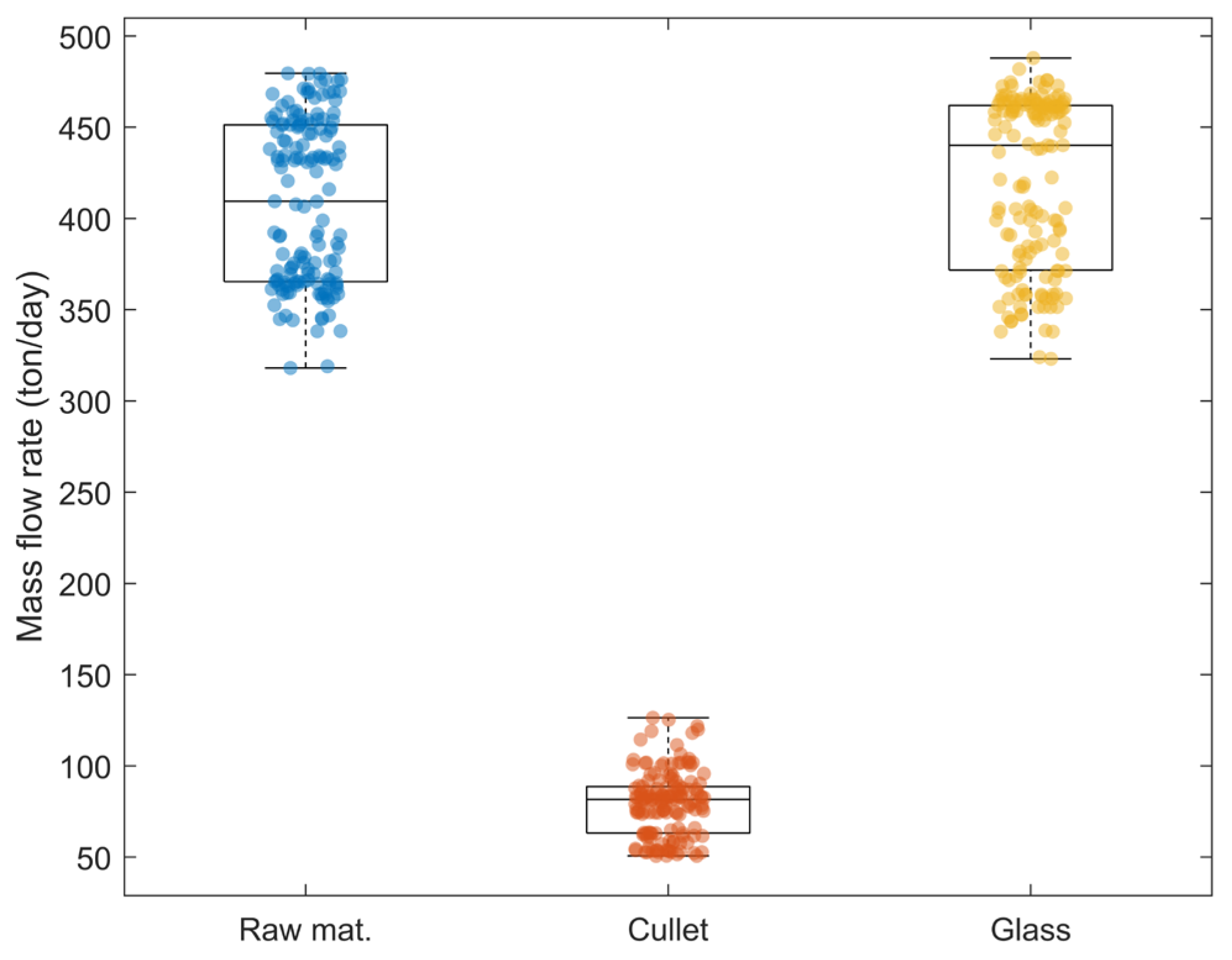
Statistical analysis involves interpreting and drawing conclusions from data. A box plot is a statistical graphic that is used to visualize the distribution of a dataset. This graphic enables a quick assessment of central tendency, variability, and potential outliers in numerical data. The box plot is based on five components: minimum value, first quartile (Q1), median (Q2), third quartile (Q3), maximum value, and outliers. Box plots of raw material, cullet, and glass are presented in Figure 3.

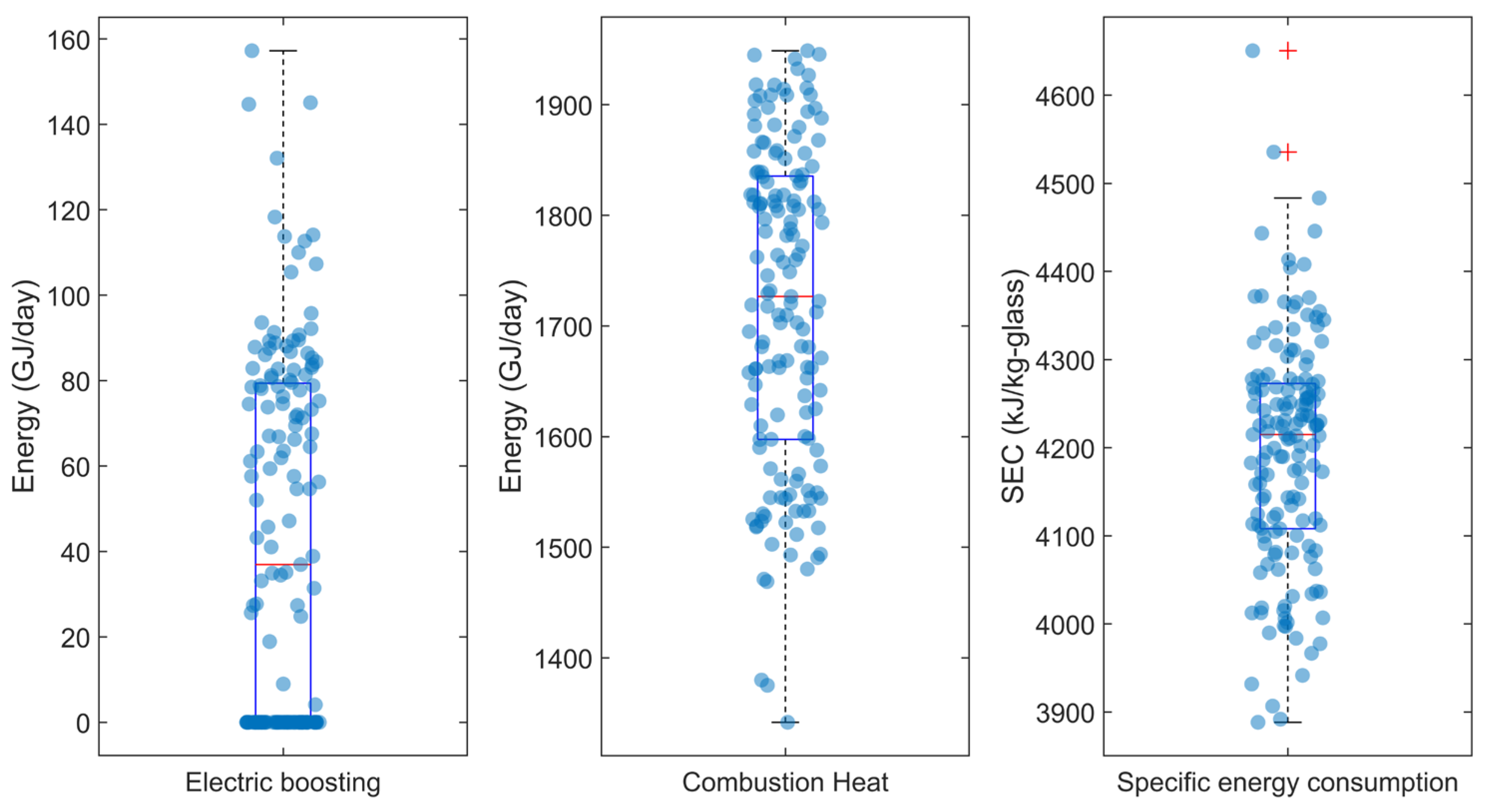
Figure 3 shows that the median values of raw material and glass are slightly higher than the mean. The raw material flow rate varies between 318.03 and 497.50 tons/day, while the cullet varies from 50.70 to 126.37 tons/day. The glass production varies between 323.06 and 488.02 tons/day. The wide variations are mainly due to the daily fluctuations in glass production orders and the changeable availability of cullet in the process. Box plots of the electric boosting, combustion heat input, and specific energy consumption are presented in Figure 4.

Figure 4 reveals that the distribution of electric boosting, combustion heat, and specific energy consumption values shows significant variation. The electric boosting ranges from 0 to 157.25 GJ/day. The combustion heat value varies between 1341.79 and 1948.81 GJ/day. Most of the energy used in the glass furnace is supplied by combustion heat (which is primarily derived from natural gas).

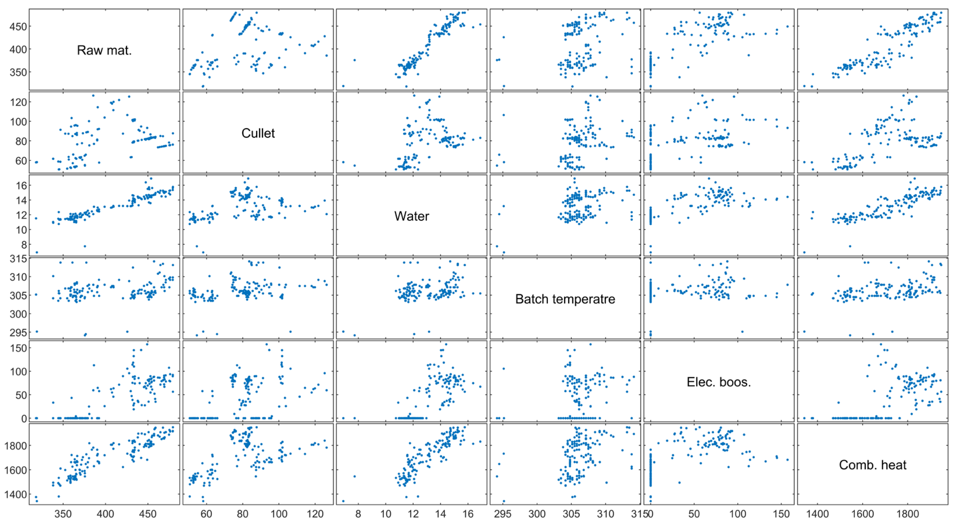
A scatter plot is a graphical tool used to represent the relationship between two quantitative variables. The X-axis corresponds to the independent variable, and the Y-axis corresponds to the dependent variable. Each data point presents an individual observation. Scatter plots are generally used for determining dataset distribution and identifying correlations (positive, negative, or unrelated) between variables. The scatter plot matrix for the variables of raw material, cullet, water, batch temperature, electric boosting, and combustion heat is presented in Figure 5.

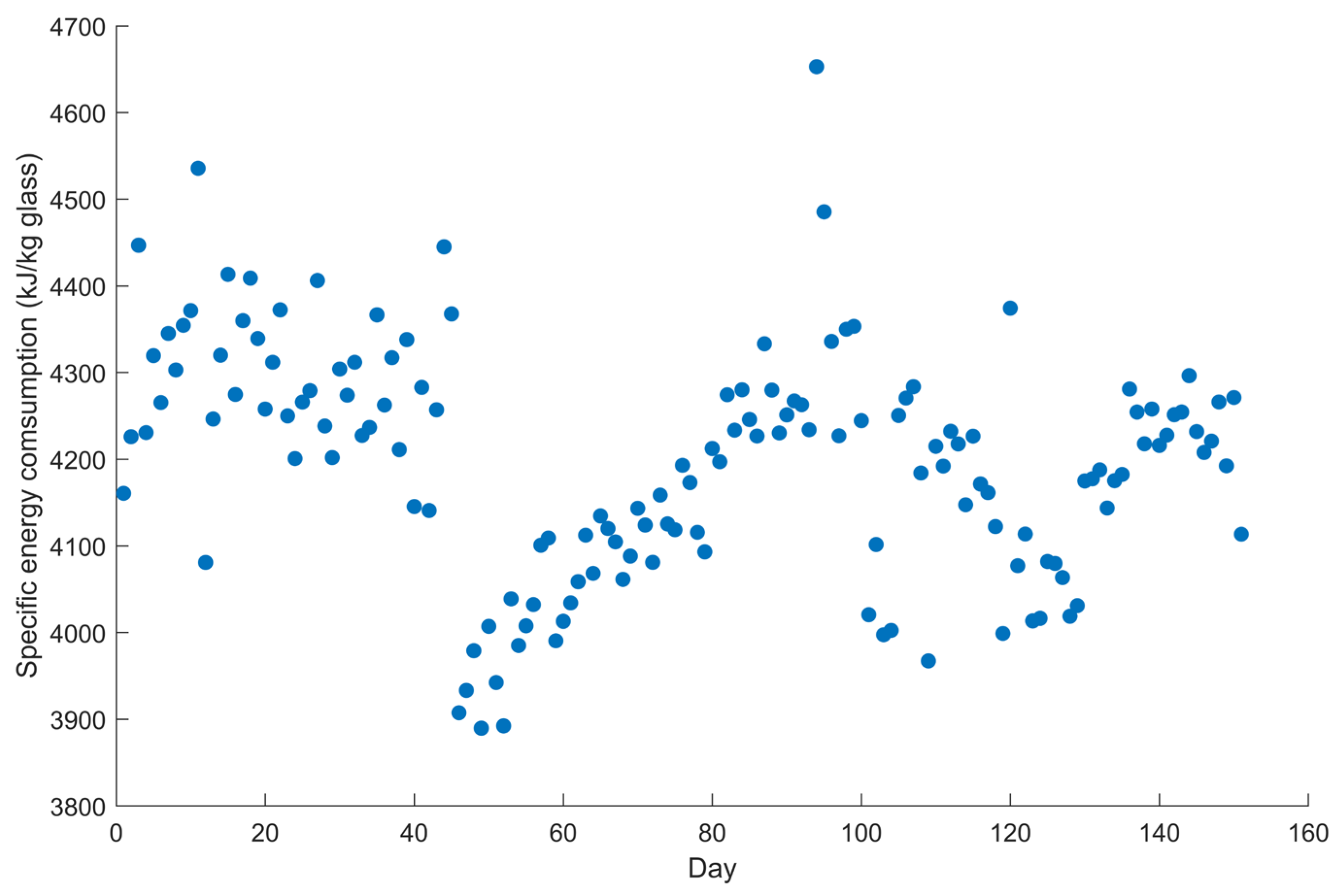
Figure 5 indicates that as the amounts of raw materials, cullet, and water increase, the required combustion heat input also increases. This increase is due to the higher glass production resulting from the increased batch input into the furnace, which in turn raises the overall energy demand. The specific energy consumption of the glass furnace for 151 days is presented in Figure 6.

When Figure 6 is examined, it is observed that specific energy consumption exhibits significant fluctuations on certain days, with some days showing notably higher values. The changes are caused by variables such as raw material, cullet, glass production, and electric boosting, which vary from day to day. These variables vary significantly depending on the daily glass production plan, furnace capacity, and factory strategy. For example, higher cullet utilization generally reduces energy demand, while increased raw material input can lead to higher combustion heat. In situations where production volume is high, cullet utilization is increased, and electrical support is used effectively, the specific energy consumption decreases.

Another significant reason for sudden changes in specific energy consumption is the disruption of stability during changes in daily production volume. Transitional periods between low and high production loads can lead to temporary increases in specific energy consumption. In this case, the glass furnace operates outside of optimal operating conditions, resulting in a decrease in furnace energy performance. These production fluctuations generally subside as the furnace adapts to the new production conditions. This adaptation involves adjusting parameters such as the internal temperature of the furnace, raw material feed rates, and electric boosting levels. However, once the production process stabilizes and the system reaches a steady-state condition, specific energy consumption returns to a normal level. This highlights the importance of maintaining production volumes as stable as possible and limiting sudden production fluctuations to improve the energy performance of glass furnaces. As a result, this dynamic structure of glass furnaces highlights the importance of monitoring and optimizing relevant parameters to improve the energy performance of glass furnaces.

3.3. Optimization Problem

This optimization problem aims to minimize the specific energy consumption of the glass furnace under certain operational constraints, using the regression model and dataset. In this way, the energy performance of the furnace can be increased by changing variables such as raw materials, cullet, and electric boosting. Also, it is possible to avoid unnecessary natural gas consumption. This approach allows for predictive decision-making in operations, contributing to both economic and environmental sustainability. Considering the operational characteristics and limitations of industrial glass furnaces, this optimization problem can be formulated as given in Equation (22) as follows:

$$\begin{gathered} \mathit{O}\mathit{b}\mathit{j}\mathit{e}\mathit{c}\mathit{t}\mathit{i}\mathit{v}\mathit{e} \mathit{f}\mathit{u}\mathit{n}\mathit{c}\mathit{t}\mathit{i}\mathit{o}\mathit{n}: \\ min {.}_{\begin{array}{c}{\dot{ m}}_{rm}, { \dot{m}}_{cul}, {\dot{ m}}_{wt},{\dot{ m}}_{fu}\\ ,{\dot{ W}}_{el}\end{array}}{SEC}_{pred}={\displaystyle \frac{{\dot{Q}}_{comb,pred}+{\dot{W}}_{el}}{{\dot{m}}_g}} \\ \mathit{s}\mathit{u}\mathit{b}\mathit{j}\mathit{e}\mathit{c}\mathit{t} \mathit{t}\mathit{o}: \\ {\dot{Q}}_{comb,pred}=RegressionModel\left({\dot{m}}_{rm},{\dot{m}}_{cul}, {\dot{m}}_{wt},T_{rm},{\dot{W}}_{el}\right) \\ {\dot{Q}}_{comb,pred}={\dot{m}}_{fu}·50027{\displaystyle \frac{\mathrm{k}\mathrm{J}}{\mathrm{k}\mathrm{g}}} \\ {\dot{m}}_g= {\dot{m}}_{rm}·{\displaystyle \frac{83.3333}{100}}+{\dot{m}}_{cul} \\ {T}_{rm}=305 \mathrm{K} \\ 0.03<{\displaystyle \frac{{\dot{m}}_{wt}}{{\dot{m}}_{rm}}}<0.037 \\ 0.14<{\displaystyle \frac{{\dot{m}}_{cul}}{{\dot{m}}_g}}<0.26 \\ 302·{10}^3\mathrm{k}\mathrm{g}<{\dot{m}}_{rm}<500·{10}^3 \mathrm{k}\mathrm{g} \\ 48·{10}^3 \mathrm{k}\mathrm{g}<{\dot{m}}_{cul}<130·{10}^3 \mathrm{k}\mathrm{g} \\ 6.91·{10}^3 \mathrm{k}\mathrm{g}<{\dot{m}}_{wt}<17.7·{10}^3 \mathrm{k}\mathrm{g} \\ 10·{10}^6 \mathrm{k}\mathrm{J}<{\dot{W}}_{el}<157·{10}^6 \mathrm{k}\mathrm{J} \\ 306·{10}^3 \mathrm{k}\mathrm{g}<{\dot{m}}_g\le 500·{10}^3 \mathrm{k}\mathrm{g} \\ 25·{10}^3 \mathrm{k}\mathrm{g}<{\dot{m}}_{fu}\le 41·{10}^3 \mathrm{k}\mathrm{g} \end{gathered}$$

(22)

The objective function of the optimization problem is the specific energy consumption. The optimization problem has four equality constraints and two inequality constraints. The decision variables include the flow rates of glass, raw materials, cullet, and water, and electric boosting. Each variable is subject to upper and lower bounds, which are incorporated into the formulation as inequality constraints.

This optimization formulation is a nonlinear nonconvex optimization problem with equality–inequality constraints. To solve this complex problem, the interior-point method was applied; the interior-point method is efficient for equality–inequality constrained optimization problems. These computations were performed on a high-performance computer to ensure timely and accurate results.

3.4. Training, Validation, and Test Data

The raw and reconciled data were divided into training, validation, and test datasets. A total of 85% of the data was allocated for cross-validation (comprising both training and validation sets), while the remaining 15% was reserved as test data to evaluate the generalization performance of the linear regression model. The split of the training, validation, and test datasets is summarized in

Table 3. Split of training, validation, and test datasets.

	Cross-Validation Dataset (85%)					Test Dataset (15%)
Split 1	Fold 1	Fold 2	Fold 3	Fold 4	Fold 5	Test data
Split 2	Fold 1	Fold 2	Fold 3	Fold 4	Fold 5
Split 3	Fold 1	Fold 2	Fold 3	Fold 4	Fold 5
Split 4	Fold 1	Fold 2	Fold 3	Fold 4	Fold 5
Split 5	Fold 1	Fold 2	Fold 3	Fold 4	Fold 5
				Training	Validation

.

3.5. Linear Regression and Optimization Using Raw Data

3.5.1. Predictor and Response Variables

The raw dataset included variables such as flow rates of raw material, cullet, water, and raw material temperatures, electric boosting, and combustion heat. The predictors and response variables obtained from the raw dataset are summarized in

Table 4. Predictor and response variables of the linear regression model (raw dataset).

Obs.	Predictor Variables					Response Variable
	${\dot{\mathit{m}}}_{\mathit{r}\mathit{m}}\left(\mathbf{t}\mathbf{o}\mathbf{n}\right)$	${\dot{\mathit{m}}}_{\mathit{c}\mathit{u}\mathit{l}}\left(\mathbf{t}\mathbf{o}\mathbf{n}\right)$	${\dot{\mathit{m}}}_{\mathit{w}\mathit{t}}\left(\mathbf{t}\mathbf{o}\mathbf{n}\right)$	${\mathit{T}}_{\mathit{r}\mathit{m}}\left(\mathbf{K}\right)$	${\dot{\mathit{W}}}_{\mathit{e}\mathit{l}}\left(\mathbf{M}\mathbf{J}\right)$	${\mathit{Q}}_{\mathit{c}\mathit{o}\mathit{m}\mathit{b}}\left(\mathbf{G}\mathbf{J}\right)$
1	430.844	63.334	13.213	305.15	47.160	1710.199
2	429.738	63.17	13.179	304.15	57.600	1722.720
3	392.440	57.702	12.453	304.817	57.600	1653.271
4	365.860	53.792	11.671	303.15	0	1517.449
5	364.585	53.592	11.691	304.817	0	1543.869
6	363.310	53.426	11.541	305.817	0	1519.247
7	363.992	52.857	11.818	305.817	0	1547.646
8	363.337	53.403	11.215	304.817	0	1532.643
9	354.729	51.533	11.493	304.15	0	1511.612
10	345.429	50.794	11.342	305.483	0	1480.396
⋮	⋮	⋮	⋮	⋮	⋮	⋮
⋮	⋮	⋮	⋮	⋮	⋮	⋮
⋮	⋮	⋮	⋮	⋮	⋮	⋮
142	471.283	74.835	15.128	309.15	78.120	1909.676
143	463.903	73.664	14.984	311.15	86.040	1872.051
144	461.899	73.345	15.119	310.817	86.400	1882.452
145	469.507	74.553	14.993	310.15	66.852	1904.408
146	475.284	78.246	14.924	309.483	107.327	1888.519
147	457.330	83.616	14.741	307.15	80.136	1881.410
148	457.358	83.593	14.727	314.15	88.070	1894.452
149	464.826	84.969	15.277	313.15	71.474	1908.703
150	467.813	84.714	15.282	313.483	80.640	1946.284
151	479.859	87.704	15.787	313.15	56.264	1949.412

.

3.5.2. Cross-Validation Results Using Raw Data

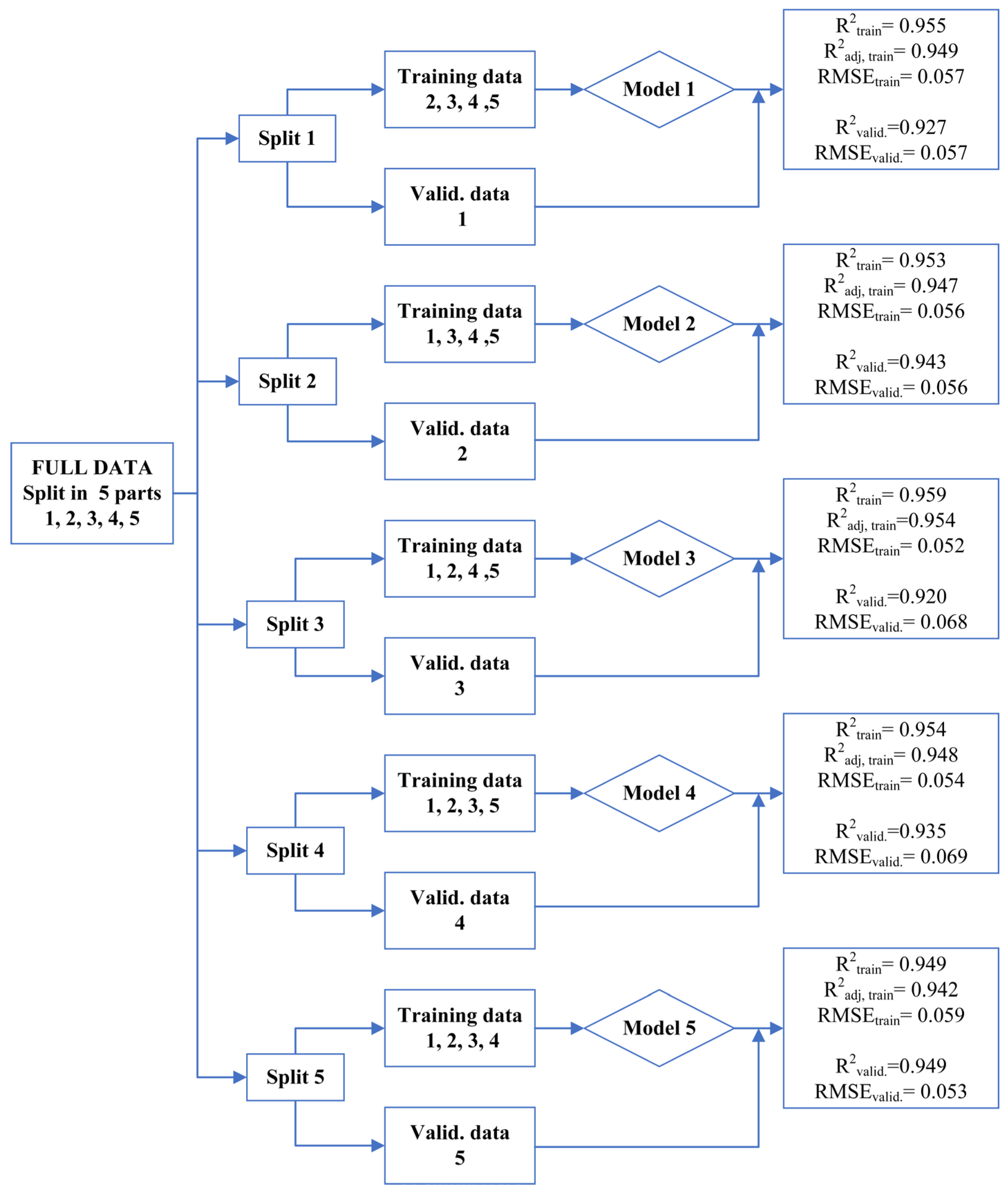
The purpose of the cross-validation technique is to determine whether a model performs consistently on different subsets of the dataset. This approach helps when evaluating the reliability of the data, detecting inconsistencies within the dataset, and mitigating the risk of the overfitting problem. To perform cross-validation, the cross-validation data were divided into five folds. A separate regression model was trained for each fold, and performance metrics including the coefficient of determination (R²) and root mean square error (RMSE) were calculated for each model, for training and validation. The results of the cross-validation analysis are presented in Figure 7.

The mean R² value obtained from the five-fold cross-validation was 0.954 with a standard deviation of 0.0039. These results show that the model demonstrated high and consistent performance on different sub-datasets. In addition, the low standard deviation enhances the generalizability of the model and suggests that it is unlikely to suffer from overfitting.

3.5.3. Stepwise Linear Regression Results

The linear regression model was created by using the min–max normalized raw training dataset. In total, 128 days of the normalized raw training data were used in the construction of this regression model. The results of stepwise linear regression with the normalized raw training dataset are presented in

Table 5. Stepwise linear regression model summary (using raw data).

Metric	Value
Observations	128
Predictors	5
Terms	12
Degree of freedom	115
Estimated coefficients (including intercept)	13
R-squared	0.953
Adjusted R-squared	0.948
Root mean squared error (RMSE)	0.0558
F-statistic vs. constant model	193
p-value	3.04·10−70
AICc	−360.03
BIC	−326.15

.

As shown in Table 5, the R-squared value was 0.953, the p-value was $3.04·{10}^{-70}$. The regression model coefficients, along with their t-statistics and p-values, are provided in

Table 6. Estimated coefficients, t-statistics, and p-values of stepwise linear regression (using normalized training raw data).

	Variables	Estimate (Coefficients ${\mathit{c}}_{\mathit{i}}$)	SE	t-Stat	p-Value
1	Intercept	−0.113	0.049	−2.334	0.021
2	${\dot{\mathit{m}}}_{\mathit{r}\mathit{m}}$	1.005	0.140	7.165	7.955·10−11
3	${\dot{\mathit{m}}}_{\mathit{c}\mathit{u}\mathit{l}}$	1.171	0.203	5.759	7.162·10−8
4	${\mathit{T}}_{\mathit{r}\mathit{m}}$	0.486	0.163	1.975	0.004
5	${\dot{\mathit{W}}}_{\mathit{e}\mathit{l}}$	−1.024	0.270	−3.785	2.455·10−4
6	${\dot{\mathit{m}}}_{\mathit{r}\mathit{m}}·{\dot{\mathit{W}}}_{\mathit{e}\mathit{l}}$	−1.726	0.279	−6.169	1.057·10−8
7	${\dot{\mathit{m}}}_{\mathit{c}\mathit{u}\mathit{l}}·{\dot{\mathit{m}}}_{\mathit{w}\mathit{t}}$	−0.629	0.272	−2.310	0.023
8	${\dot{\mathit{m}}}_{\mathit{c}\mathit{u}\mathit{l}}·{\mathit{T}}_{\mathit{r}\mathit{m}}$	−0.824	0.239	−3.446	7.961·10−4
9	${\dot{\mathit{m}}}_{\mathit{w}\mathit{t}}·{\mathit{T}}_{\mathit{r}\mathit{m}}$	−0.877	0.313	−2.83	0.005
10	${\dot{\mathit{m}}}_{\mathit{w}\mathit{t}}·{\dot{\mathit{W}}}_{\mathit{e}\mathit{l}}$	1.858	0.460	4.042	9.163·10−5
11	${\mathit{T}}_{\mathit{r}\mathit{m}}·{\dot{\mathit{W}}}_{\mathit{e}\mathit{l}}$	0.853	0.229	3.725	3.038·10−5
12	${\dot{\mathit{m}}}_{\mathit{r}\mathit{m}}^2$	0.416	0.143	2.907	0.0004
13	${\mathit{T}}_{\mathit{r}\mathit{m}}^2$	0.236	0.104	2.266	0.023

.

The equation corresponding to the stepwise regression model (using training normalized raw data, n presents that the variable is normalized), as detailed in Table 6, is given in Equation (23).

$$\begin{array}{c}{\dot{\mathit{Q}}}_{\mathit{c}\mathit{o}\mathit{m}\mathit{b},\mathit{p}\mathit{r}\mathit{e}\mathit{d},\mathit{n}}({\dot{\mathit{m}}}_{\mathit{r}\mathit{m},\mathit{n}},{\dot{\mathit{m}}}_{\mathit{c}\mathit{u}\mathit{l},\mathit{n}}, {\dot{\mathit{m}}}_{\mathit{w}\mathit{t},\mathit{n}}, {\mathit{T}}_{\mathit{r}\mathit{m},\mathit{n}}, {\dot{\mathit{W}}}_{\mathit{e}\mathit{l},\mathit{n}})\\ =-0.113+1.005·{\dot{\mathit{m}}}_{\mathit{r}\mathit{m},\mathit{n}}+1.171·{\dot{\mathit{m}}}_{\mathit{c}\mathit{u}\mathit{l},\mathit{n}}+0.486·{\mathit{T}}_{\mathit{r}\mathit{m},\mathit{n}}\\ - 1.024·{\dot{\mathit{W}}}_{\mathit{e}\mathit{l},\mathit{n}}-1.726·{\dot{\mathit{m}}}_{\mathit{r}\mathit{m},\mathit{n}}·{\dot{\mathit{W}}}_{\mathit{e}\mathit{l},\mathit{n}}-0.629·{\dot{\mathit{m}}}_{\mathit{c}\mathit{u}\mathit{l},\mathit{n}}·{\dot{\mathit{m}}}_{\mathit{w}\mathit{t},\mathit{n}}\\ - 0.824·{\dot{\mathit{m}}}_{\mathit{c}\mathit{u}\mathit{l},\mathit{n}}·{\mathit{T}}_{\mathit{r}\mathit{m},\mathit{n}}-0.877·{\dot{\mathit{m}}}_{\mathit{w}\mathit{t},\mathit{n}}·{\mathit{T}}_{\mathit{r}\mathit{m},\mathit{n}}+1.858·{\dot{\mathit{m}}}_{\mathit{w}\mathit{t},\mathit{n}}\\ ·{\dot{\mathit{W}}}_{\mathit{e}\mathit{l},\mathit{n}}+0.853·{\mathit{T}}_{\mathit{r}\mathit{m},\mathit{n}}·{\dot{\mathit{W}}}_{\mathit{e}\mathit{l},\mathit{n}}+0.416·{\dot{\mathit{m}}}_{\mathit{r}\mathit{m},\mathit{n}}^2+0.236·{\mathit{T}}_{\mathit{r}\mathit{m},\mathit{n}}^2\end{array}$$

(23)

The final model equation in real physical units, obtained by denormalizing Equation (23) using the formula $\mathit{X}=(X_{mın}+{\mathit{X}}_{\mathit{n}\mathit{o}\mathit{r}\mathit{m}}\cdot \left(X_{max}-X_{min}\right))$, is shown in Equation (24).

$$\begin{array}{c}{\dot{\mathit{Q}}}_{\mathit{c}\mathit{o}\mathit{m}\mathit{b},\mathit{p}\mathit{r}\mathit{e}\mathit{d}}({\dot{\mathit{m}}}_{\mathit{r}\mathit{m}},{\dot{\mathit{m}}}_{\mathit{c}\mathit{u}\mathit{l}}, {\dot{\mathit{m}}}_{\mathit{w}\mathit{t}}, {\mathit{T}}_{\mathit{r}\mathit{m}}, {\dot{\mathit{W}}}_{\mathit{e}\mathit{l}})\\ =15112268188.538-2370.375·{\dot{\mathit{m}}}_{\mathit{r}\mathit{m}}+110266.965·{\dot{\mathit{m}}}_{\mathit{c}\mathit{u}\mathit{l}}\\ + 817418.537·{\dot{\mathit{m}}}_{\mathit{w}\mathit{t}}-160454113.033·{\mathit{T}}_{\mathit{r}\mathit{m}}-44.271·{\dot{\mathit{W}}}_{\mathit{e}\mathit{l}}\\ - 0.00004124·{\dot{\mathit{m}}}_{\mathit{r}\mathit{m}}·{\dot{\mathit{W}}}_{\mathit{e}\mathit{l}}-0.5043·{\dot{\mathit{m}}}_{\mathit{c}\mathit{u}\mathit{l}}·{\dot{\mathit{m}}}_{\mathit{w}\mathit{t}}-331.037\\ ·{\dot{\mathit{m}}}_{\mathit{c}\mathit{u}\mathit{l}}·{\mathit{T}}_{\mathit{r}\mathit{m}}-2691.999·{\dot{\mathit{m}}}_{\mathit{w}\mathit{t}}·{\mathit{T}}_{\mathit{r}\mathit{m}}+0.0007168·{\dot{\mathit{m}}}_{\mathit{w}\mathit{t}}·{\dot{\mathit{W}}}_{\mathit{e}\mathit{l}}\\ + 0.1648·{\mathit{T}}_{\mathit{r}\mathit{m}}·{\dot{\mathit{W}}}_{\mathit{e}\mathit{l}}+0.009663·{\dot{\mathit{m}}}_{\mathit{r}\mathit{m}}^2+357999.670·{\mathit{T}}_{\mathit{r}\mathit{m}}^2\end{array}$$

(24)

Table 6 reveals that all of the p-values in the model are less than 0.05. The regression model developed from the training raw dataset was evaluated by comparing the predicted values with the observed values. The results of this comparison are illustrated in Figure 8.

3.5.4. Testing of the Linear Regression Model Using the Test Part of the Raw Dataset

The linear regression model developed using the training data was evaluated on the test dataset. The main objective of this testing phase was to assess how accurately the model’s predictions aligned with the actual (unseen) data. This step also provides insights into the model’s generalizability and its potential applicability in real-world scenarios. The results of the model when applied to the test data are presented in

Table 7. Result table of test data using the trained stepwise linear regression model (using raw data).

Metric	Value
Number of test data (measurements)	23
Coefficient of determination $R^2$	0.9494
Root mean squared error RMSE	0.0427

.

The R-squared value of the raw test dataset (0.949) is very close to that of the raw training dataset (0.953), which indicates that the model does not suffer from overfitting and maintains a high level of predictive accuracy on unseen data. In order to evaluate the prediction performance of the regression model on the test data, the actual values (observations), estimated values (model estimations), and relative errors of combustion heat were calculated and are presented in

Table 8. Calculated and predicted combustion heat values along with relative errors for the test raw dataset.

Day	Calculated Value (GJ)	Predicted Values (GJ)	Residuals (GJ)	Relative Error (%)
4	1517.449	1534.271	−16.822	−1.109
19	1544.393	1570.806	−26.413	−1.71
28	1573.512	1605.429	−31.917	−2.028
47	1681.889	1701.627	−19.738	−1.174
58	1819.022	1802.033	16.989	0.934
61	1758.187	1774.302	−16.115	−0.917
63	1813.265	1811.334	1.931	0.106
72	1794.414	1837.852	−43.438	−2.421
78	1831.412	1856.864	−25.452	−1.39
79	1830.558	1878.218	−47.660	−2.604
84	1836.319	1804.824	31.495	1.715
102	1661.532	1686.556	−25.024	−1.506
108	1637.141	1645.519	−8.378	−0.512
110	1625.414	1636.156	−10.742	−0.661
113	1662.466	1646.759	15.707	0.945
119	1719.157	1760.48	−41.323	−2.404
121	1729.802	1748.467	−18.665	−1.079
125	1818.869	1798.601	20.268	1.114
128	1772.604	1796.232	−23.628	−1.333
134	1856.716	1862.396	−5.680	−0.306
145	1904.408	1928.309	−23.901	−1.255
147	1881.41	1846.511	34.899	1.855
151	1949.412	1978.228	−28.816	−1.478

.

Table 8 reports that the relative error in predicting the combustion heat required by the glass furnace ranged from a minimum of 0.106% to a maximum of 2.604%, with the most errors around 1.328% (mean absolute error). The relative error between the actual and predicted combustion heat value may have been caused by a sudden change in daily glass production. If the daily glass production requirement of the furnace had been a little more stable, the value of the relative error that the model would have made may perhaps have been even lower. In addition, accurately knowing the daily combustion heat requirement before production begins allows precise estimation of the amount of natural gas needed from the network and its cost.

These results demonstrate that the regression model has robust predictive capability. The small difference between training and test R² values confirms that the model captures the underlying process dynamics effectively and can be applied confidently for energy performance optimization in glass furnaces.

3.5.5. The Solution of the Optimization Problem with Raw Data

The optimization problem was solved using the interior-point method. The minimum specific energy consumption and the corresponding optimal values of the decision variables are presented in

Table 9. Optimal specific energy consumption and corresponding input variables.

	Variable	Optimal Values
Decision variable	Raw material	469.063 ton/day
	Cullet	109.114 ton/day
	Water	14.072 ton/day
	Batch temperature	305 K
	Electric boosting	157.000 GJ/day
	Fuel	33.435 ton/day
Minimum value of the objective function	Specific energy consumption	$\mathbf{3659.30} {\displaystyle \frac{\mathbf{k}\mathbf{J}}{\mathbf{k}\mathbf{g} \mathbf{g}\mathbf{l}\mathbf{a}\mathbf{s}\mathbf{s}}}$
Other information	Pulled glass	500.000 ton/day
	Combustion heat from natural gas	1672.652 GJ/day
	Humidity	0.030

.

Table 9 indicates that the optimization problem yields the best minimum specific energy consumption when solved using the interior-point method. It is observed that as the amount of produced molten glass increases, the specific energy consumption of the glass furnace also increases. Also, the lower humidity in the raw material is provided to increase energy consumption.

3.6. Linear Regression and Constrained Optimization Using Reconciled Data

In this section, the reconciled dataset is normalized. A linear regression model is then created using the normalized reconciled data. This linear regression model, created with the training normalized reconciled data, is then denormalized using the denormalization method. This regression model is then optimized for the specific energy consumption of this furnace using certain constraints and optimization methods.

3.6.1. Predictor and Response Variables

The reconciled dataset includes variables such as flow rates of raw material, cullet, water, and raw material temperatures, and electric boosting. The response variable is combustion heat. These predictors and response variables, which are obtained from reconciled data, are summarized in

Table 10. Predictor and response variables of the linear regression model (reconciled dataset).

Obs.	Predictor Variables					Response Variable
	${\dot{\mathit{m}}}_{\mathit{r}\mathit{m}}\left(\mathbf{t}\mathbf{o}\mathbf{n}\right)$	${\dot{\mathit{m}}}_{\mathit{c}\mathit{u}\mathit{l}}\left(\mathbf{t}\mathbf{o}\mathbf{n}\right)$	${\dot{\mathit{m}}}_{\mathit{w}\mathit{t}}\left(\mathbf{t}\mathbf{o}\mathbf{n}\right)$	${\mathit{T}}_{\mathit{b}\mathit{a}\mathit{t}\mathit{c}\mathit{h}}\left(\mathbf{K}\right)$	${\dot{\mathit{W}}}_{\mathit{e}\mathit{l}}\left(\mathbf{M}\mathbf{J}\right)$	${\mathit{Q}}_{\mathit{c}\mathit{o}\mathit{m}\mathit{b}}\left(\mathbf{G}\mathbf{J}\right)$
1	430.807	63.334	13.192	305.137	47.159	1709.956
2	429.694	63.171	13.159	304.133	57.598	1722.394
3	392.426	57.704	12.436	304.795	57.598	1652.839
4	365.853	53.794	11.653	303.152	0	1517.534
5	364.595	53.595	11.675	304.808	0	1543.739
6	363.296	53.428	11.524	305.813	0	1519.224
7	364.002	52.859	11.801	305.802	0	1547.538
8	363.349	53.406	11.200	304.812	0	1532.594
9	354.742	51.536	11.477	304.144	0	1511.530
10	345.447	50.797	11.326	305.476	0	1480.292
⋮	⋮	⋮	⋮	⋮	⋮	⋮
⋮	⋮	⋮	⋮	⋮	⋮	⋮
⋮	⋮	⋮	⋮	⋮	⋮	⋮
142	471.206	74.834	15.105	309.120	78.115	1908.992
143	463.816	73.663	14.960	311.120	86.034	1871.391
144	461.832	73.344	15.096	310.785	86.393	1881.761
145	469.425	74.552	14.970	310.120	66.849	1903.743
146	474.913	78.236	14.904	309.453	107.318	1887.885
147	457.226	83.614	14.719	307.122	80.131	1880.772
148	457.239	83.589	14.705	314.118	88.064	1893.757
149	464.740	84.967	15.254	313.120	71.470	1908.044
150	467.726	84.712	15.259	313.451	80.635	1945.546
151	479.4956	87.691	15.767	313.122	56.262	1948.807

.

3.6.2. Cross-Validation Results Using Training Reconciled Data

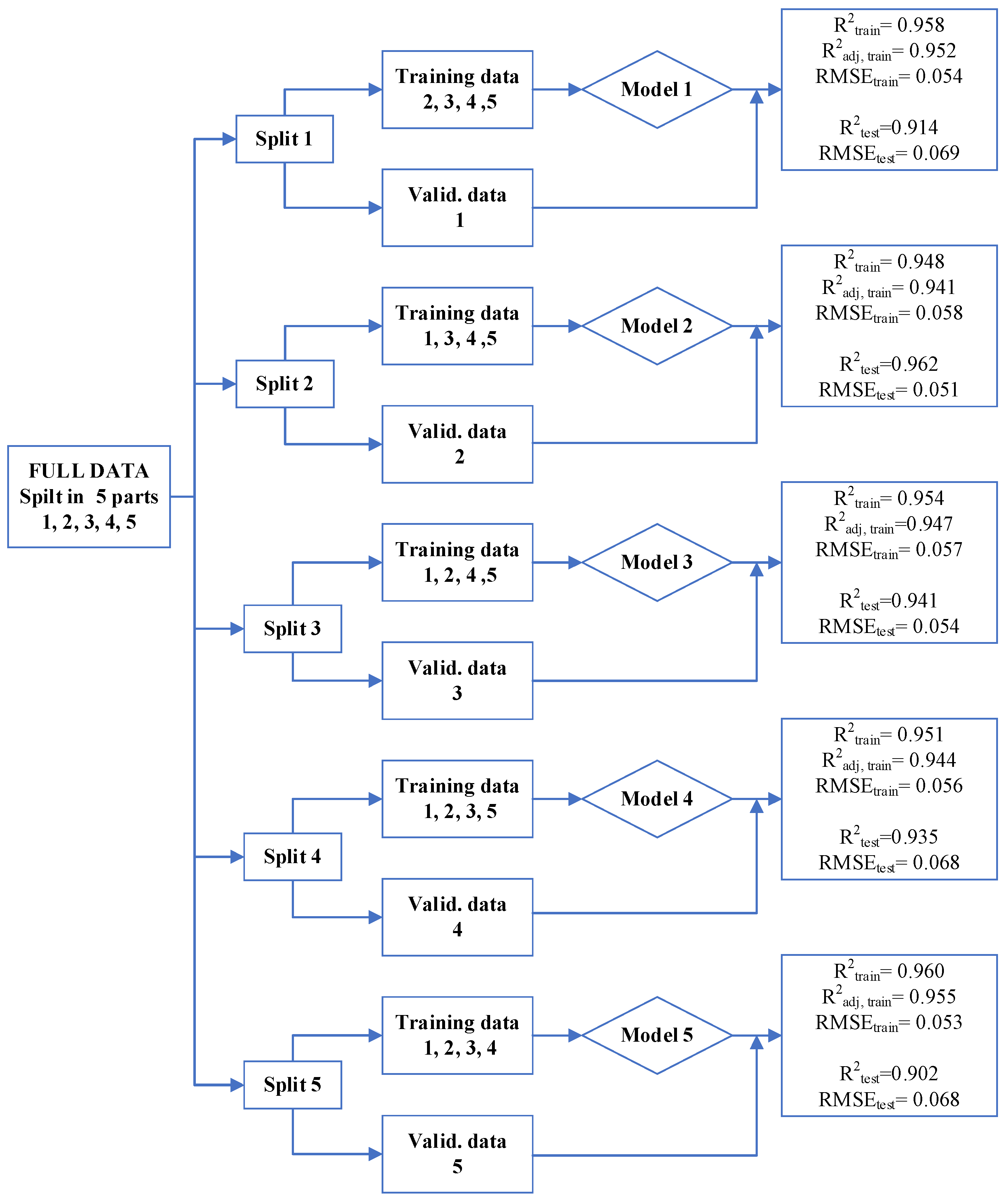
The cross-validation data (reconciled dataset) were divided into five sets. The results of the cross-validation analysis are presented in Figure 9.

The mean R² value obtained from the five-fold cross-validation is 0.9542 with a standard deviation of 0.0050. The closeness of these R² values provides important information about the generalizability of the model. These results show that the model demonstrates high and consistent performance on different sub-datasets.

3.6.3. Stepwise Linear Regression Results

The linear regression model was created using min–max training normalized reconciled data. In total, 128 days of normalized reconciled data were used in the construction of this regression model. The reason for using normalized data as regression data was to both increase the regression model and obtain more accurate and reliable results. The results of stepwise linear regression with normalized reconciled data are presented in

Table 11. Stepwise linear regression model summary (using reconciled data).

Metric	Value
Observations	128
Predictors	5
Terms	12
Degree of freedom	115
Estimated coefficients (including intercept)	13
R-squared	0.9529
Adjusted R-squared	0.9480
Root mean squared error (RMSE)	0.05576
F-statistic vs. constant model	193.81
p-value	2.71·10−70
AICc	−360.22
BIC	−326.34

.

As shown in Table 11, the R-squared value is 0.953, the p-value value is 2.1·10⁻⁸⁵. The regression model coefficients, along with their t-statistics and p-values, are provided in

Table 12. Estimated coefficients, t-statistics, and p-values of stepwise linear regression (using normalized reconciled data).

	Variables	Estimate (Coefficients ${\mathit{c}}_{\mathit{i}}$)	SE	t-Stat	p-Value
1	Intercept	−0.114	0.049	−2.333	0.0214
2	${\dot{\mathit{m}}}_{\mathit{r}\mathit{m}}$	1.002	0.140	7.153	8.477·10−11
3	${\dot{\mathit{m}}}_{\mathit{c}\mathit{u}\mathit{l}}$	1.173	0.203	5.772	6.765·10−8
4	${\mathit{T}}_{\mathit{r}\mathit{m}}$	0.485	0.163	2.269	0.003
5	${\dot{\mathit{W}}}_{\mathit{e}\mathit{l}}$	−1.025	0.271	−3.791	2.407·10−4
6	${\dot{\mathit{m}}}_{\mathit{r}\mathit{m}}·{\dot{\mathit{W}}}_{\mathit{e}\mathit{l}}$	−1.729	0.279	−6.187	9.685·10−9
7	${\dot{\mathit{m}}}_{\mathit{c}\mathit{u}\mathit{l}}·{\dot{\mathit{m}}}_{\mathit{w}\mathit{t}}$	−0.629	0.272	−2.312	0.023
8	${\dot{\mathit{m}}}_{\mathit{c}\mathit{u}\mathit{l}}·{\mathit{T}}_{\mathit{r}\mathit{m}}$	−0.825	0.239	−3.454	7.74·10−4
9	${\dot{\mathit{m}}}_{\mathit{w}\mathit{t}}·{\mathit{T}}_{\mathit{r}\mathit{m}}$	−0.886	0.3137	−2.824	0.005
10	${\dot{\mathit{m}}}_{\mathit{w}\mathit{t}}·{\dot{\mathit{W}}}_{\mathit{e}\mathit{l}}$	1.861	0.459	4.049	9.374·10−5
11	${\mathit{T}}_{\mathit{r}\mathit{m}}·{\dot{\mathit{W}}}_{\mathit{e}\mathit{l}}$	0.853	0.229	3.732	2.964·10−4
12	${\dot{\mathit{m}}}_{\mathit{r}\mathit{m}}^2$	0.418	0.142	2.929	0.004
13	${\mathit{T}}_{\mathit{r}\mathit{m}}^2$	0.234	0.104	2.258	0.026

.

The equation corresponding to the stepwise regression model (using normalized reconciled data), as detailed in Table 12, is given in Equation (25).

$$\begin{array}{c}{\dot{\mathit{Q}}}_{\mathit{c}\mathit{o}\mathit{m}\mathit{b},\mathit{p}\mathit{r}\mathit{e}\mathit{d},\mathit{n}}({\dot{\mathit{m}}}_{\mathit{r}\mathit{m},\mathit{n}},{\dot{\mathit{m}}}_{\mathit{c}\mathit{u}\mathit{l},\mathit{n}}, {\dot{\mathit{m}}}_{\mathit{w}\mathit{t},\mathit{n}}, {\mathit{T}}_{\mathit{r}\mathit{m},\mathit{n}}, {\dot{\mathit{W}}}_{\mathit{e}\mathit{l},\mathit{n}})\\ =-0.114+1.002·{\dot{\mathit{m}}}_{\mathit{r}\mathit{m},\mathit{n}}+1.173·{\dot{\mathit{m}}}_{\mathit{c}\mathit{u}\mathit{l},\mathit{n}}+0.485·{\mathit{T}}_{\mathit{r}\mathit{m},\mathit{n}}\\ - 1.025·{\dot{\mathit{W}}}_{\mathit{e}\mathit{l},\mathit{n}}-1.729·{\dot{\mathit{m}}}_{\mathit{r}\mathit{m},\mathit{n}}·{\dot{\mathit{W}}}_{\mathit{e}\mathit{l},\mathit{n}}-0.629·{\dot{\mathit{m}}}_{\mathit{c}\mathit{u}\mathit{l},\mathit{n}}·{\dot{\mathit{m}}}_{\mathit{w}\mathit{t},\mathit{n}}\\ - 0.825·{\dot{\mathit{m}}}_{\mathit{c}\mathit{u}\mathit{l},\mathit{n}}·{\mathit{T}}_{\mathit{r}\mathit{m},\mathit{n}}-0.886·{\dot{\mathit{m}}}_{\mathit{w}\mathit{t},\mathit{n}}·{\mathit{T}}_{\mathit{r}\mathit{m},\mathit{n}}+1.861·{\dot{\mathit{m}}}_{\mathit{w}\mathit{t},\mathit{n}}\\ ·{\dot{\mathit{W}}}_{\mathit{e}\mathit{l},\mathit{n}}+0.853·{\mathit{T}}_{\mathit{r}\mathit{m},\mathit{n}}·{\dot{\mathit{W}}}_{\mathit{e}\mathit{l},\mathit{n}}+0.418·{\dot{\mathit{m}}}_{\mathit{r}\mathit{m},\mathit{n}}^2+0.234·{\mathit{T}}_{\mathit{r}\mathit{m},\mathit{n}}^2\end{array}$$

(25)

The final model equation in real physical units, obtained by denormalizing Equation (25) using the formula $\mathit{X}=(X_{mın}+{\mathit{X}}_{\mathit{n}\mathit{o}\mathit{r}\mathit{m}}·\left(X_{max}-X_{min}\right))$, is shown in Equation (26).

$$\begin{array}{c}{\dot{\mathit{Q}}}_{\mathit{c}\mathit{o}\mathit{m}\mathit{b},\mathit{p}\mathit{r}\mathit{e}\mathit{d}}({\dot{\mathit{m}}}_{\mathit{r}\mathit{m}},{\dot{\mathit{m}}}_{\mathit{c}\mathit{u}\mathit{l}}, {\dot{\mathit{m}}}_{\mathit{w}\mathit{t}}, {\mathit{T}}_{\mathit{r}\mathit{m}}, {\dot{\mathit{W}}}_{\mathit{e}\mathit{l}})\\ =15100191150.950-2423.072·{\dot{\mathit{m}}}_{\mathit{r}\mathit{m}}+110356.787·{\dot{\mathit{m}}}_{\mathit{c}\mathit{u}\mathit{l}}\\ + 817618.734·{\dot{\mathit{m}}}_{\mathit{w}\mathit{t}}-159682403.878·{\mathit{T}}_{\mathit{r}\mathit{m}}-44.286·{\dot{\mathit{W}}}_{\mathit{e}\mathit{l}}\\ - 0.00004132·{\dot{\mathit{m}}}_{\mathit{r}\mathit{m}}·{\dot{\mathit{W}}}_{\mathit{e}\mathit{l}}-0.5049·{\dot{\mathit{m}}}_{\mathit{c}\mathit{u}\mathit{l}}·{\dot{\mathit{m}}}_{\mathit{w}\mathit{t}}-331.331\\ ·{\dot{\mathit{m}}}_{\mathit{c}\mathit{u}\mathit{l}}·{\mathit{T}}_{\mathit{r}\mathit{m}}-2692.621·{\dot{\mathit{m}}}_{\mathit{w}\mathit{t}}·{\mathit{T}}_{\mathit{r}\mathit{m}}+0.0007185·{\dot{\mathit{m}}}_{\mathit{w}\mathit{t}}·{\dot{\mathit{W}}}_{\mathit{e}\mathit{l}}\\ + 0.1649·{\mathit{T}}_{\mathit{r}\mathit{m}}·{\dot{\mathit{W}}}_{\mathit{e}\mathit{l}}+0.0097329·{\dot{\mathit{m}}}_{\mathit{r}\mathit{m}}^2+356653.138\\ ·{\mathit{T}}_{\mathit{r}\mathit{m}}^2\end{array}$$

(26)

Table 12 shows that all of the p-values in the model are less than 0.05, indicating that these variables are statistically significant. In general, the high adjusted R-squared value (94.9%) and significant F-statistic of the model indicate that the independent variables explain the dependent variable quite well. This situation confirms that the selected variables and model structure successfully capture the effects on the process. As a result, the obtained model quantitatively reveals the effects of glass furnace process parameters and provides important information for glass furnaces.

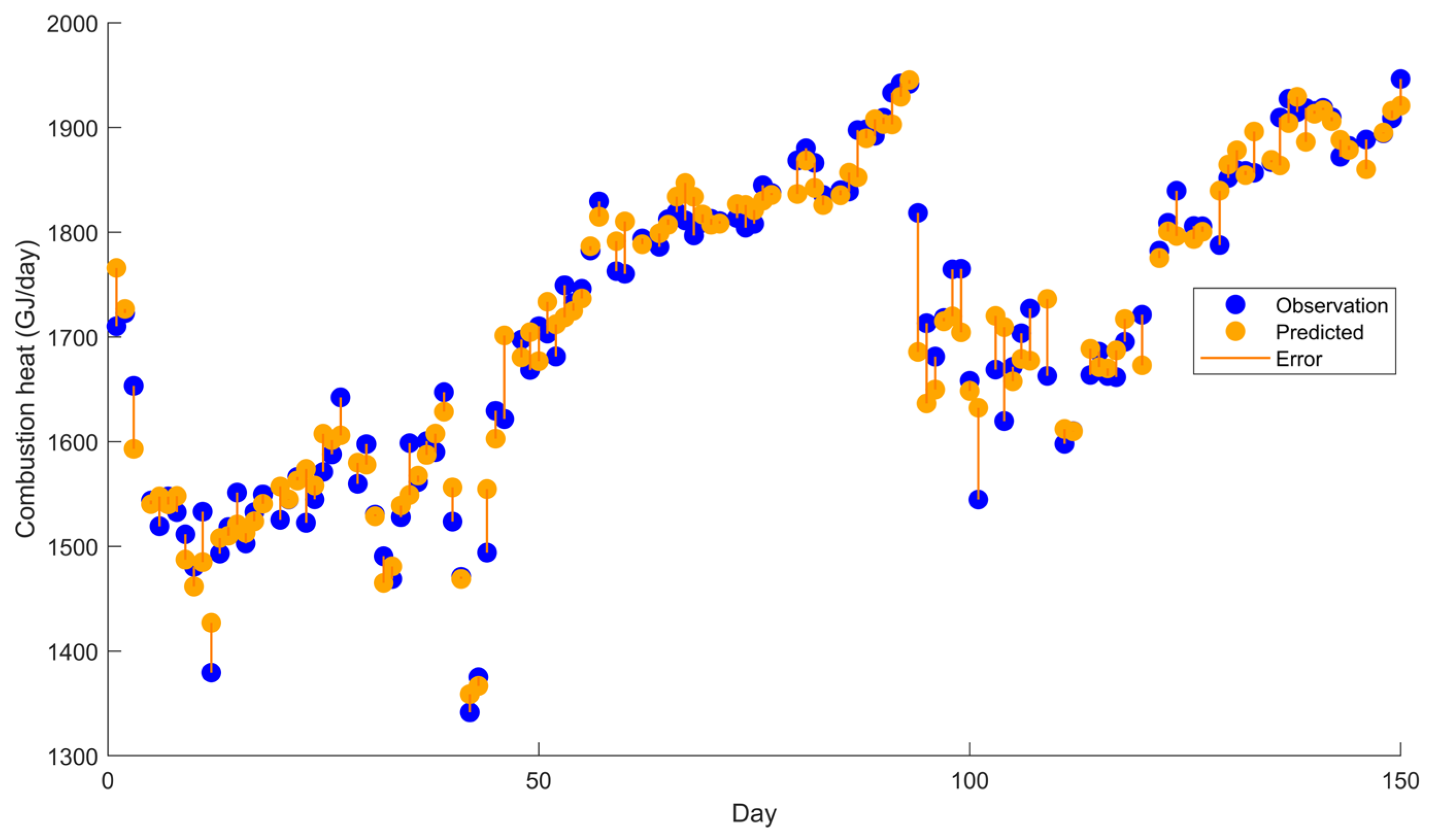
The model developed using the reconciled dataset was evaluated by comparing the predicted values with the actual values. In this analysis, the predictive performance of the model is assessed by comparing the observed values, the corresponding predicted values, and the associated prediction errors. The results of this comparison are illustrated in Figure 10.

The linear regression model gives results very close to the actual values. Furthermore, the prediction errors are relatively small, indicating a strong model fit. These results suggest that the model has high predictive capability and can be reliably used in further energy optimization studies. The accuracy of the model also indicates that the selected predictor variables are highly relevant to combustion heat behavior in glass furnaces.

3.6.4. Testing of Linear Regression Model Using the Test Part of the Reconciled Dataset

The linear regression model developed using the training data was evaluated on the test dataset. The linear regression model was developed using training data and tested on the test dataset. The test results are presented in

Table 13. Result table of test data using the trained stepwise linear regression model (using reconciled data).

Metric	Value
Number of test data (observation)	23
Coefficient of determination $R^2$	0.9496
Root mean squared error RMSE	0.0426

.

The R² value of the test dataset (0.9496) is quite close to the R-squared value of the training dataset (0.955), indicating that the model avoids overfitting and provides high levels of prediction accuracy. The relative errors for the prediction performance of the model on the test part of the reconciled dataset, based on actual and predicted values, were obtained and are summarized in

Table 14. Reconciled and predicted combustion heat values along with relative errors, obtained using the test part of the reconciled dataset.

Day ID	Reconciled Value (GJ)	Predicted Values (GJ)	Residuals (GJ)	Relative Error (%)
4	1517.534	1534.395	−16.861	−1.111
19	1544.178	1570.578	−26.400	−1.71
28	1573.444	1605.124	−31.680	−2.013
47	1681.612	1700.471	−18.859	−1.122
58	1818.38	1801.976	16.404	0.902
61	1757.617	1774.097	−16.480	−0.938
63	1812.635	1811.242	1.393	0.077
72	1794.155	1838.038	−43.883	−2.446
78	1831.054	1856.606	−25.552	−1.396
79	1830.146	1877.802	−47.656	−2.604
84	1835.767	1804.485	31.282	1.704
102	1661.284	1686.461	−25.177	−1.516
108	1636.882	1645.125	−8.243	−0.504
110	1625.1	1635.404	−10.304	−0.634
113	1662.097	1646.183	15.914	0.957
119	1718.951	1760.216	−41.265	−2.401
121	1729.365	1748.249	−18.884	−1.092
125	1818.342	1798.407	19.935	1.096
128	1772.272	1796.17	−23.898	−1.348
134	1856.135	1861.653	−5.518	−0.297
145	1903.743	1927.793	−24.050	−1.263
147	1880.772	1845.945	34.827	1.852
151	1948.807	1976.607	−27.800	1.401

.

According to Table 14, the relative error in estimating the required combustion heat for a glass furnace ranged from 0.077% to 2.994%, with nearly all errors around 1.322% (mean absolute error). These errors could be due to the sudden fluctuations in glass production. More stable glass production may lead to low relative error. As can be seen from the results, the regression model demonstrates robust prediction capability, as evidenced by the R² value.

3.6.5. The Solution of the Optimization Problem with Reconciled Data

The optimization problem was solved using the interior-point method. The minimum specific energy consumption and the corresponding optimal values of the decision variables are presented in

Table 15. Optimal specific energy consumption and corresponding input variables obtained from the interior-point method algorithm.

	Variable	Optimal Values
Decision variable	Raw material	468.769 ton/day
	Cullet	109.359 ton/day
	Water	14.063 ton/day
	Batch temperature	305 K
	Electric boosting	157.000 GJ/day
	Fuel	33.443 ton/day
Minimum value of the objective function	Specific energy consumption	$\mathbf{3660.088} {\displaystyle \frac{\mathbf{k}\mathbf{J}}{\mathbf{k}\mathbf{g} \mathbf{g}\mathbf{l}\mathbf{a}\mathbf{s}\mathbf{s}}}$
Other information	Pulled glass	5000.000 ton/day
	Combustion heat from natural gas	1673.044 GJ/day
	Humidity	0.030

.

As detailed in Table 15, the optimal solution was obtained under nonlinear inequality constraints using the interior-point method. The specific energy consumption value (3660.088 ${\displaystyle \frac{\mathrm{kJ}}{\mathrm{kg} \mathrm{glass}}}$) reported here corresponds to the lowest achievable energy consumption while satisfying all process constraints. When Table 15 is examined, it can be observed that as the amount of produced molten glass increases, the specific energy consumption of the glass furnace also increases. This outcome reflects the increasing energy demand required to maintain thermal efficiency during high-capacity operation. Moreover, it should be noted that the value of electric boosting is close to its upper operational limit, which suggests that maximizing electric assistance plays a critical role in optimizing energy performance under constrained conditions. Additionally, the minimum SEC obtained is consistent with the values reported in the literature and is considered a reasonable and realistic result for industrial-scale glass furnaces. Furthermore, based on the developed model, when the electric boosting power is kept constant, the relationship between raw material and cullet flow rates becomes an important factor in determining combustion heat demand.

3.7. Comparison of Regression Model and Optimization Results Using Raw Data and Reconciled Data

The metrics of the linear regression models and optimization results obtained with raw data and reconciled data are given in

Table 16. Comparison of linear regression and optimization results with raw data and reconciled data.

		Metric	Raw Data	Reconciled Data
Linear regression	Cross-validation	Mean R-squared	0.9545 ± 0.0039	0.9542 ± 0.0050
		Mean RMSE	0.054	0.0058
	Final model	R-squared	0.9528	0.9529
		Adjusted R-squared	0.9479	0.9480
		Root mean squared error (RMSE)	0.05581	0.05576
		F-statistic vs. constant model	193.40	193.80
		p-value	3.04·10−70	2.71·10−71
		AICc	−360.03	−360.20
		BIC	−326.15	−326.04
	Test of final model	R-squared	0.9494	0.9496
		RMSE	0.0427	0.0426
Optimization		Specific energy consumption	$3659.30{\displaystyle \frac{\mathrm{k}\mathrm{J}}{\mathrm{k}\mathrm{g} \mathrm{g}\mathrm{l}\mathrm{a}\mathrm{s}\mathrm{s}}}$	$3660.088{\displaystyle \frac{\mathrm{k}\mathrm{J}}{\mathrm{k}\mathrm{g} \mathrm{g}\mathrm{l}\mathrm{a}\mathrm{s}\mathrm{s}}}$

.

Comparing the regression and optimization results (Table 16) obtained using raw and reconciled data reveals that the regression model built with reconciled data yields more reliable results. Lower p-values, RMSE, AICc, and BIC metrics were obtained with the reconciled data. In the optimization results, the lowest specific energy consumption was 3659.30 kJ/kg glass with the raw data, while it was 3660.088 kJ/kg glass with the reconciled data. If a specific energy consumption analysis had been conducted using only the raw data, we would have found a lower specific energy consumption value than expected, which would have been misleading. However, using reconciled data prevented this misleading error, and a more reliable specific energy consumption result was obtained. In summary, using reconciled data instead of raw data both increased the reliability of the linear regression model and helped achieve more reliable optimization results. As a result, better results for optimizing furnace performance were obtained by creating a linear regression model and using reconciled data.

3.8. Graphical Analysis of Specific Energy Consumption Dependency on Raw Material and Cullet (with Reconciled Data)

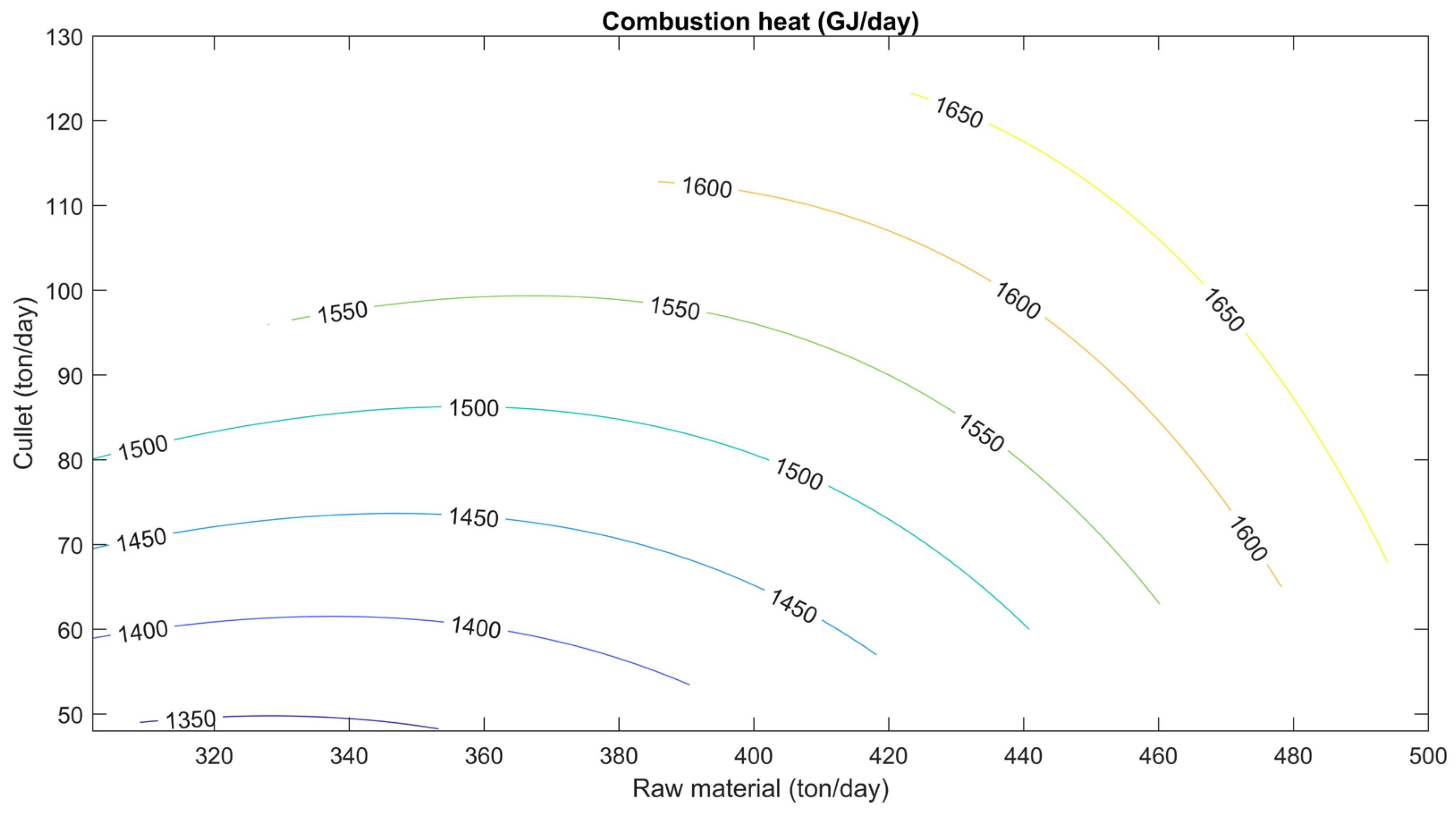
In this section, the effects of raw material and cullet consumption on the specific energy consumption of a glass furnace are investigated, assuming certain optimal points that minimize specific energy consumption in the optimization problem. These constants were met under the following conditions: a humidity (water/raw material ratio) of 0.03, a raw material temperature of 305 K, electric boosting of 157 GJ, and a maximum glass production capacity of 500 tons. The combustion heat requirement of the glass furnace under these conditions is given in Figure 11.

As can be seen from Figure 11, when the amounts of raw materials and cullet increase, the combustion heat required by the glass furnace also rises. This is expected, as processing larger quantities of material demands greater thermal input to maintain melting efficiency and quality.

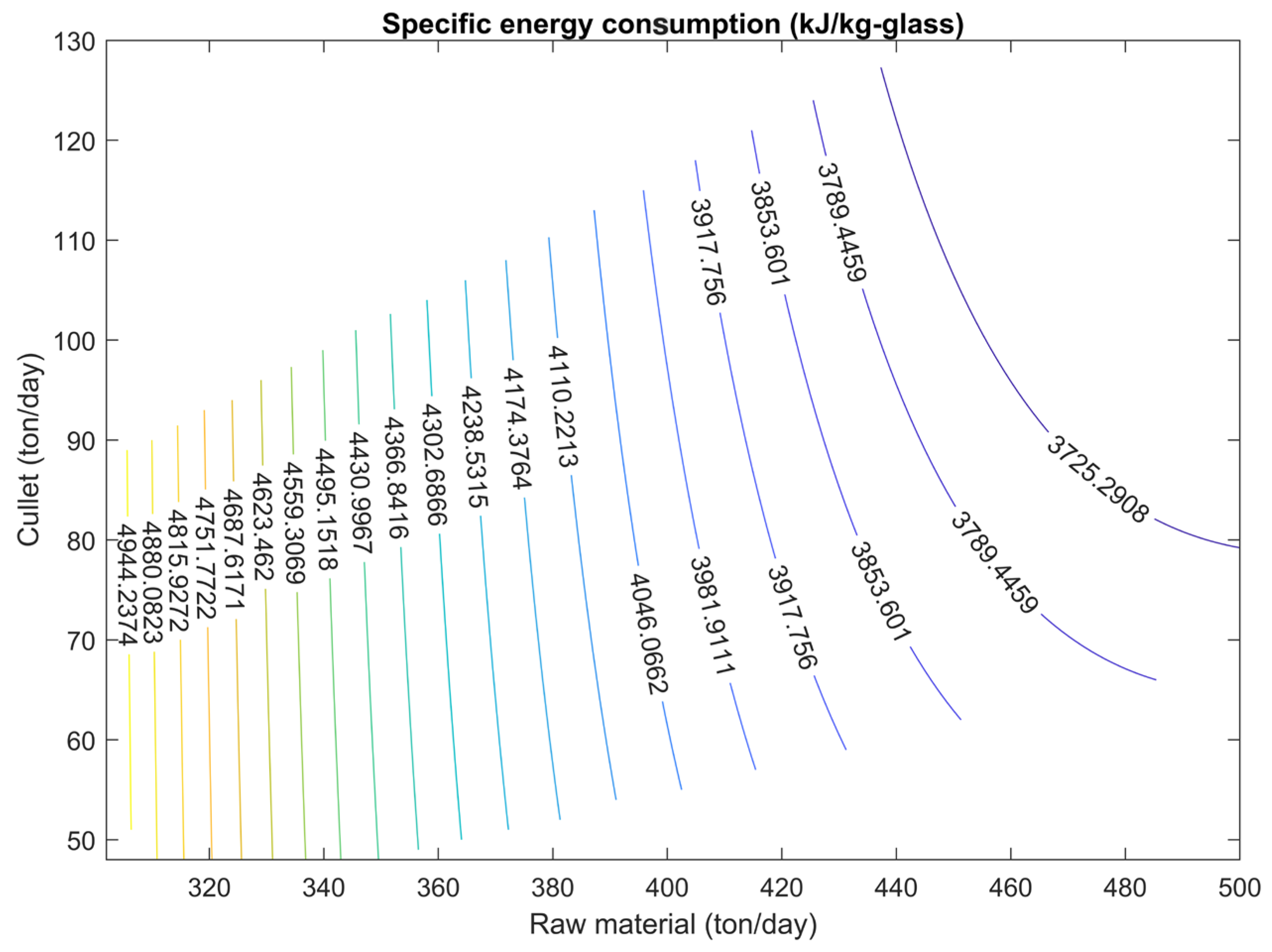
The estimated specific energy consumption as a function of raw material and cullet inputs under this condition is illustrated in Figure 12 (contour plot with level curves). These visualizations help to better understand how material input combinations influence energy performance and to identify operating points that yield lower specific energy consumption values.

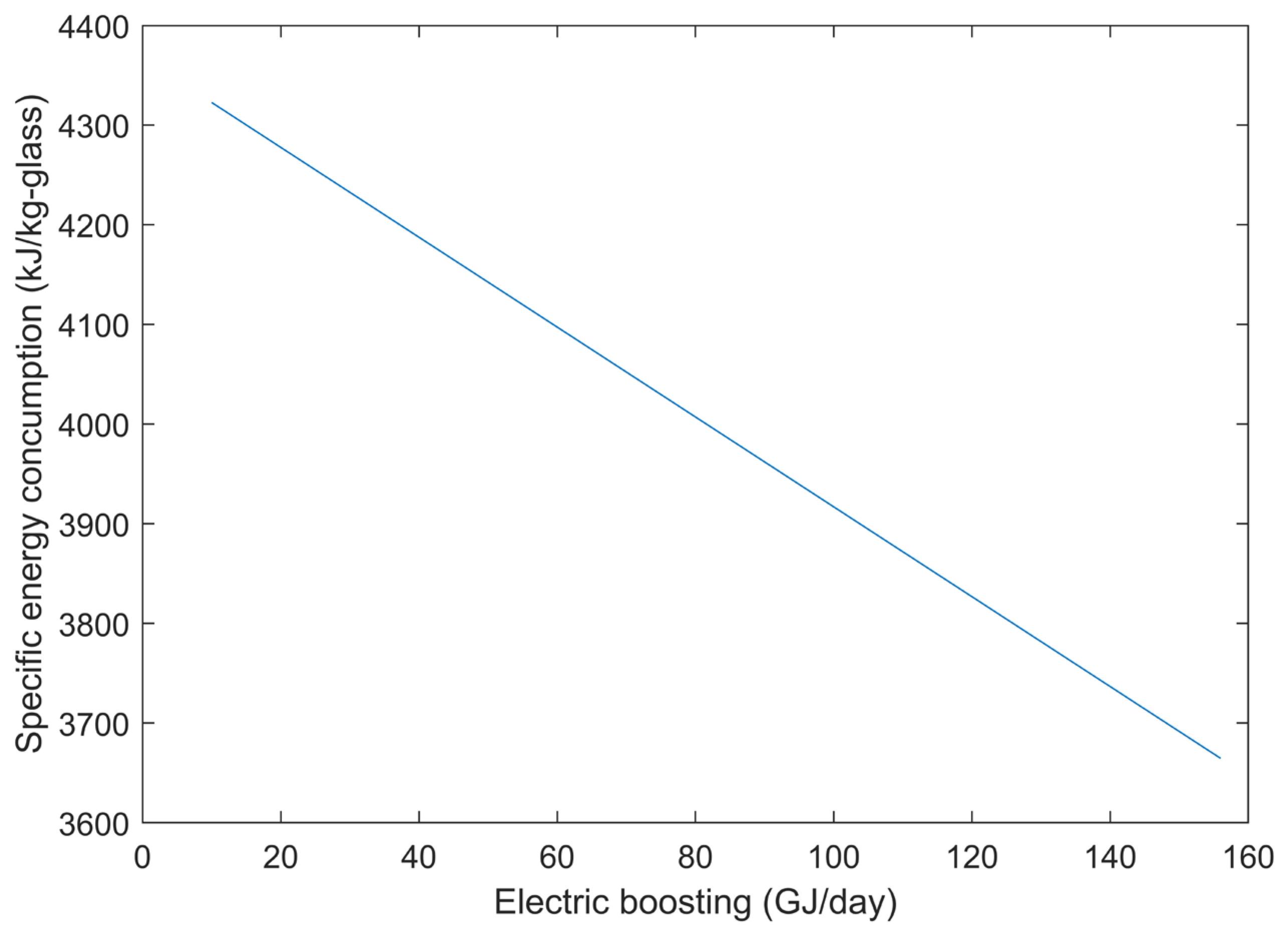
Figure 12 illustrates that as the flow rates of raw materials and cullet rise, the specific energy of the glass furnace decreases. An important observation is that despite the increase in daily glass production associated with these higher input rates, the specific energy consumption of the glass furnace decreases, indicating improved energy efficiency at larger production scales. These findings highlight the model’s capability not only to optimize energy use but also to provide reliable, precise predictions of the furnace’s energy demand (combustion heat) with minimal error margins, based on varying daily production requirements. Such insights are critical for operational planning and cost reduction in glass manufacturing. The effect of electric boosting on specific energy consumption is given by Figure 13.

Figure 13 illustrates that the specific energy consumption of the glass melting furnace is strongly affected by changes in electric boosting. According to Figure 13, an increase in electric boosting adversely affects the specific energy consumption. However, the adverse linear trend indicates that achieving higher electric boosting rates can contribute to a more efficient melting process. This is because heat transfer from electric boosting to the glass bath is more effective than that from fuel combustion over the glass bath. Consequently, the energy requirement per unit mass of glass decreases steadily as the electric boosting increases.

This finding highlights the positive impact of electric boosting on the overall energy performance of the furnace. When the findings and results are examined, this study demonstrates that the energy performance of glass furnaces can be significantly improved through the integration of data reconciliation, statistical modeling, and advanced optimization methods. Furthermore, even a slight improvement in energy performance, particularly in energy-intensive glass furnaces, results in significant fuel savings. The stepwise linear regression model employed in this study explains a significant portion of the variation in combustion heat demand. Furthermore, this regression model provides high prediction accuracy with both the training and test data sets. The use of reconciled process data and cross-validation also increases model reliability and prevents overfitting. Furthermore, it is demonstrated that specific energy consumption can be effectively reduced using various optimization algorithms under certain operational constraints. Among the optimization methods tested, the interior-point algorithm provided the most efficient solution with the lowest specific energy consumption.

The most striking of these results is that specific energy consumption decreases significantly as cullet flow rate, glass production, and the amount of electric boosting increase. It is also worth discussing the suggestion that if global glass factories built fewer furnaces and produced glass at full capacity instead of operating at half capacity, the specific energy consumption of these glass furnaces would decrease significantly (Figure 12), because the furnaces are designed for full capacity but are operated at half capacity. Currently, significant efforts are being made to improve the energy performance of glass furnaces. In addition to this effort, it is understood that operating glass furnaces at near full capacity can significantly improve their energy performance. When planning for the future, it is crucial to operate existing furnaces at full capacity rather than overbuilding. This will reduce specific energy consumption and avoid the cost of installing additional furnaces.

3.9. Limitations

The primary objective of this study is to predict and subsequently optimize the energy performance of a glass furnace based on various input variables. However, there are certain physical limitations inherent to this process. These limitations include the following:

• The data obtained from the glass furnaces are aggregated daily rather than being instantaneous. In future, collecting minute- or hour-based data is expected to enable more detailed and accurate analyses.
• The raw material typically remains inside the furnace for approximately 24 h; however, due to internal circulation, individual material batches do not exit the furnace simultaneously. Therefore, calculations are performed using the average residence time.
• Due to the extremely high temperatures within the furnace, data cannot be gathered uniformly from all regions. To address the missing measurements, data reconciliation methods are employed to estimate these unmeasured variables.

4. Conclusions

In this study, to optimize the specific energy consumption of a glass furnace, the effects of critical variables such as raw material, cullet, water, raw material temperature, and electrical energy were investigated quantitatively. The findings show that increasing the raw material and cullet flow rate and using electric boosting significantly increased the energy performance of the furnace. Furthermore, the regression model obtained by using reconciled data via data reconciliation rather than raw data was proven to provide more reliable and consistent results in the optimization process.

The main contributions and key findings of this research study are as follows. When comparing two different linear regression models, the model created with the reconciled data ($R_{training}^2=0.9529 and R_{test}^2=0.9496$) was found to be much more reliable. Afterwards, the most reliable optimization results were obtained with reconciled data. The minimum specific energy consumption was found to be 3660.088 $\mathrm{k}\mathrm{J}/\mathrm{k}\mathrm{g} \mathrm{g}\mathrm{l}\mathrm{a}\mathrm{s}\mathrm{s}$ using the interior-point method, under optimized process conditions. When the glass furnace operates at partial capacity instead of full capacity, the furnace uses more energy. Overall, the specific energy consumption of glass furnaces may be effectively decreased through optimizing production parameters, increasing electric boosting usage and the cullet ratio, and nearly full capacity operation. The findings of this study offer important implications for both the glass furnace studied and other industrial processes involving similar energy intensity. The demonstration that specific energy consumption can be reduced through accurate modeling and optimization techniques provides a critical framework for industrial efficiency and sustainability.

Future studies could involve real-time or high-frequency data collection to analyze transient behavior more accurately. Furthermore, hybrid modeling approaches that combine process-based models and statistical data-driven models to take advantage of their complementary strengths could be employed to better capture the furnace’s dynamic performance. Finally, integrating the optimization framework with techno-economic and environmental analysis considering parameters such as energy cost and CO₂ emissions would enable a more sustainable assessment of glass furnace operations.

References

1. Sardeshpande, V.; Gaitonde, U.N.; Banerjee, R. Model based energy benchmarking for glass furnace. Energy Convers. Manag. 2007, 48, 2718–2738. [Google Scholar] [CrossRef]
2. Sardeshpande, V.; Anthony, R.; Gaitonde, U.N.; Banerjee, R. Performance analysis for glass furnace regenerator. Appl. Energy 2011, 88, 4451–4458. [Google Scholar] [CrossRef]
3. Zier, M.; Stenzel, P.; Kotzur, L.; Stolten, D. A Review of decarbonization options for the glass industry. Energy Convers. Manag. X 2021, 10, 100083. [Google Scholar] [CrossRef]
4. Miserocchi, L.; Franco, A.; Testi, D. Status and prospects of energy efficiency in the glass industry: Measuring, Assessing and Improving Energy Performance. Energy Convers. Manag. X 2024, 24, 100720. [Google Scholar] [CrossRef]
5. Furszyfer Del Rio, D.D.; Sovacool, B.K.; Foley, A.M.; Griffiths, S.; Bazilian, M.; Kim, J.; Rooney, D. Decarbonizing the glass industry: A Critical and Systematic Review of Developments, Sociotechnical Systems and Policy Options. Renew. Sustain. Energy Rev. 2022, 155, 111885. [Google Scholar] [CrossRef]
6. Atzori, D.; Tiozzo, S.; Vellini, M.; Gambini, M.; Mazzoni, S. Industrial technologies for CO2 reduction applicable to glass furnaces. Thermo 2023, 3, 682–710. [Google Scholar] [CrossRef]
7. Canbaz, E.D.; Gür, M. Machine-learning-based reduced order modeling for operational analysis of industrial glass melting furnaces using CFD solutions. Isı Bilim. Tek. Derg. 2025, 45, 56–68. [Google Scholar] [CrossRef]
8. Kodak, O.; Sadeghi-Khaneghah, F.; Kaya, M.B.; Kılıç, L.; Arzan, N.; Dumankaya, E.; Alanat, G.Y.; Konukman, A.E.S. Evaluation of electrically boosted natural gas fired glass furnace performance by using data reconciliation method. Heliyon 2025, 11, e42624. [Google Scholar] [CrossRef]
9. Raič, J.; Wachter, P.; Hödl, P.; Demuth, M.; Gaber, C.; Gerhardter, H.; Prieler, R.; Hochenauer, C. CFD simulation aided glass quality and energy efficiency analysis of an oxy-fuel glass melting furnace with electric boosting. Energy Convers. Manag. X 2022, 15, 100252. [Google Scholar] [CrossRef]
10. Conradt, R. Prospects and physical limits of processes and technologies in glass melting. J. Asian Ceram. Soc. 2019, 7, 377–396. [Google Scholar] [CrossRef]
11. Mastropasqua, L.; Drago, F.; Chiesa, P.; Giuffrida, A. Oxygen transport membranes for efficient glass melting. Membranes 2020, 10, 442. [Google Scholar] [CrossRef]
12. Han, J.; Li, L.; Wang, J.; Chen, S.; Liu, C.; Li, C. Simulation and evaluation of float glass furnace with different electrode positions. J. Am. Ceram. Soc. 2022, 105, 7097–7110. [Google Scholar] [CrossRef]
13. Romero, M.; Robla, J.I.; Padilla, I.; García-Hierro, J.; López-Delgado, A. Eco-efficient melting of glass frits by concentrated solar energy. Sol. Energy 2018, 174, 321–327. [Google Scholar] [CrossRef]
14. Liu, T.-I.; Lyons, C.S.; Sukanya, S.; Yang, C.-H. Intelligent measurements for monitoring and control of glass production furnace for green and efficient manufacturing. Int. J. Adv. Manuf. Technol. 2014, 75, 339–349. [Google Scholar] [CrossRef]
15. Cravero, C.; Spoladore, A. Transient numerical simulation of regenerative systems with waste gas recirculation strategies in glass production plant. Appl. Sci. 2019, 9, 1496. [Google Scholar] [CrossRef]
16. Beknazaryan, D.V.; Kanewets, G.E.; Strogonov, K.V. Efficiency criteria for thermal insulation structures of glass furnaces. J. Sib. Fed. Univ. Eng. Technol. 2021, 14, 459–471. [Google Scholar] [CrossRef]
17. Weidner, T.; Galán-Martín, Á.; Ryberg, M.W.; Guillén-Gosálbez, G. Energy systems modeling and optimization for absolute environmental sustainability: Current landscape and opportunities. Comput. Chem. Eng. 2022, 164, 107883. [Google Scholar] [CrossRef]
18. Beerkens, R.G.C.; Van Limpt, H.A.C.; Jacobs, G. Energy efficiency benchmarking of glass furnaces. Glass Sci. Technol. 2002, 77, 47–57. [Google Scholar] [CrossRef]
19. Fellaou, S.; Bounahmidi, T. Mass balance reconciliation for bilinear systems: A case study of a raw mill separator in a typical moroccan cement plant. Eng. Technol. Appl. Sci. Res. 2016, 6, 1006–1009. [Google Scholar] [CrossRef]
20. Tong, H.; Crowe, C.M. Detection of gross erros in data reconciliation by principal component analysis. AIChE J. 1995, 41, 1712–1722. [Google Scholar] [CrossRef]
21. Zhou, D.; Huang, D.; Zhang, L.; Hao, J.; Ma, S. A global thermodynamic measurement data reconciliation model considering boundary conditions and parameter correlations and its applications to natural gas compressors. Measurement 2021, 172, 108972. [Google Scholar] [CrossRef]
22. Raič, J.; Gaber, C.; Wachter, P.; Demuth, M.; Gerhardter, H.; Knoll, M.; Prieler, R.; Hochenauer, C. Validation of a coupled 3d cfd simulation model for an oxy-fuel cross-fired glass melting furnace with electric boosting. Appl. Therm. Eng. 2021, 195, 117166. [Google Scholar] [CrossRef]
23. Wang, Z.; Liu, R.; Liu, Q.; Thompson, J.S.; Kadoch, M. Energy-efficient data collection and device positioning in UAV-Assisted IoT. IEEE Internet Things J. 2020, 7, 1122–1139. [Google Scholar] [CrossRef]
24. Xie, S.; Wang, H.; Peng, J. Energy efficiency analysis and optimization of industrial processes based on a novel data reconciliation. IEEE Access 2021, 9, 47436–47451. [Google Scholar] [CrossRef]
25. Adhi, T.P.; Saputro, U.E. Data reconciliation and gross error detection for troubleshooting of ammonia reactor. MATEC Web Conf. 2018, 156, 03029. [Google Scholar] [CrossRef]
26. Yuan, Y.; Khatibisepehr, S.; Huang, B.; Li, Z. Bayesian method for simultaneous gross error detection and data reconciliation. AIChE J. 2015, 61, 3232–3248. [Google Scholar] [CrossRef]
27. Dumont, O.; Quoilin, S.; Lemort, V. Importance of the reconciliation method to handle experimental data in refrigeration and power cycle: Application to a reversible heat pump/organic rankine cycle unit integrated in a positive energy building. Int. J. Energy Environ. Eng. 2016, 7, 137–143. [Google Scholar] [CrossRef]
28. Li, L.; Lin, H.-J.; Han, J.; Ruan, J.; Xie, J.; Zhao, X. Three-dimensional glass furnace model of combustion space and glass tank with electric boosting. Mater. Trans. 2019, 60, 1034–1043. [Google Scholar] [CrossRef]
29. Li, L.; Han, J.; Lin, H.; Ruan, J.; Wang, J.; Zhao, X. Simulation of glass furnace with increased production by increasing fuel supply and introducing electric boosting. Int. J. Appl. Glass Sci. 2020, 11, 170–184. [Google Scholar] [CrossRef]
30. Ma, J.-Y.; Xia, L.; Li, Q.-L. Optimal energy-efficient policies for data centers through sensitivity-based optimization. Discret. Event. Dyn. Syst. 2019, 29, 567–606. [Google Scholar] [CrossRef]
31. Fialko, N.; Stepanova, A.; Navrodska, R.; Shevchuk, S. Optimization of geometric parameters and analysis of exergy efficiency of heat recovery units glass furnaces. Energy Autom. 2021, 3, 5–17. [Google Scholar] [CrossRef]
32. Ren, L.; Wang, H. Parameter optimization and performance comparison of several power cycles for waste heat recovery from moderate temperature flue gas. Energy Procedia 2017, 142, 1333–1339. [Google Scholar] [CrossRef]
33. Reddy, V.; P, G. Revised beaconing glowworm swarm optimization ant colony optimization algorithm to localize nodes and optimize the energy consumed by nodes in wireless sensor networks. Concurr. Comput. 2022, 34, e6013. [Google Scholar] [CrossRef]
34. Basso, D.; Cravero, C.; Reverberi, A.; Fabiano, B. CFD analysis of regenerative chambers for energy efficiency improvement in glass production plants. Energies 2015, 8, 8945–8961. [Google Scholar] [CrossRef]
35. Li, M. The Optimal Product Transition in Glass Furnaces. Ind. Eng. Chem. Res. 2009, 48, 2598–2604. [Google Scholar] [CrossRef]
36. Hu, P.; Li, Y.; Zhang, X.; Guo, Z.; Zhang, P. CO2 emission from container glass in China, and emission reduction strategy analysis. Carbon Manag. 2018, 9, 303–310. [Google Scholar] [CrossRef]
37. Özyurt, D.B.; Pike, R.W. Theory and practice of simultaneous data reconciliation and gross error detection for chemical processes. Comput. Chem. Eng. 2004, 28, 381–402. [Google Scholar] [CrossRef]
38. Romagnoli, J.A.; Sánchez, M.C. Data Processing and Reconciliation for Chemical Process Operations; Elsevier: San Diego, CA, USA, 1999; Volume 2, ISBN 9780080530277. [Google Scholar]
39. Draper, N.R.; Smith, H. Applied Regression Analysis; Wiley Series in Probability and Statistics; Wiley: Hoboken, NJ, USA, 1998; ISBN 9780471170822. [Google Scholar]
Figure 1. Schematic overview of glass furnaces [8].
Processes 13 03739 g001
Figure 2. Optimization process of glass furnace.
Processes 13 03739 g002
Figure 3. Box plots of the mass flow rates of raw material, cullet, and glass.
Processes 13 03739 g003
Figure 4. Box plots of combustion heat, electric boosting, and specific energy consumption.
Processes 13 03739 g004
Figure 5. Scatter plot matrix illustrating the relationships between dependent and independent variables.
Processes 13 03739 g005
Figure 6. Variation of specific energy consumption over 151 days.
Processes 13 03739 g006
Figure 7. Cross-validation results of the stepwise linear regression model using the training raw dataset (average R2train = 0.954, standard deviation of this σ = 0.0039).
Processes 13 03739 g007
Figure 8. Comparison of observed and predicted values with prediction error (using the training raw dataset).
Processes 13 03739 g008
Figure 9. Cross-validation results of the stepwise linear regression model using training reconciled data (average R2train = 0.9542, standard deviation of this σ = 0.0050).
Processes 13 03739 g009
Figure 10. Comparison of actual and predicted values with prediction error (using the training reconciled dataset).
Processes 13 03739 g010
Figure 11. Relationship between raw material–cullet and combustion heat demand under fixed electric boosting (157 GJ/day) and production constraints.
Processes 13 03739 g011
Figure 12. Specific energy consumption with respect to raw material and cullet input rates under fixed electric boosting (157 GJ/day).
Processes 13 03739 g012
Figure 13. Specific energy consumption with respect to electric boosting under conditions of fixed raw material (468.769 ton/day) and cullet (109.359 ton/day).
Processes 13 03739 g013