Modeling of Surfactant Enhanced Drying of Polymeric Coatings Using Random Forest Regressor

Abstract

Surfactant-based drying of polymeric coatings is a highly non-linear complex process due to the involvement of simultaneous heat and mass transfer. It is quite challenging to model this type of system mathematically. We resorted to a data-driven technique to model this type of system. A potent machine learning approach called the random forest (RF) regressor was introduced in this work to model the drying of poly(styrene)-p-xylene coatings improved by surfactants. This model was developed using experimental data. A substantial number of samples were collected by conducting experiments at a wide range of operating conditions. Apart from the accuracy of predicting coating weight loss for given values of inputs, model performance was also evaluated for the variation in the number of samples, and feature extraction was also done, which is an additional advantage of the random forest. Our results demonstrate that the random forest model trained with 80% samples is able to predict coating weight loss with less than $\pm 0.5\%$ error, and even a model trained with just 20% samples is able to predict the remaining 80% samples with just $\pm 2\%$ error. It also outperformed the regression tree and the artificial neural network (ANN) used in previous studies for the same dataset.

1. Introduction

Polymeric coatings are widely used in food, electronics, textile, and automotive industries as protective layers that prevent cracking, moisture ingress, and degradation, thereby enhancing durability. These coatings are typically formed by depositing polymeric solutions onto substrates. Although organic solvent-based coatings are common, their environmental and health hazards have driven a shift toward water-based alternatives, which are more sustainable and biocompatible; however, the lower volatility of water results in slower drying and higher energy requirements [1].

Many commercial coatings incorporate crystalline or glassy polymers to enhance strength, rigidity, and functional stability. The drying process involves coupled heat and mass transfer along a moving boundary, accompanied by phase transitions such as rubbery-to-glassy and sol–gel transformations [1]. Surfactants can accelerate this process by modifying interfacial properties, and the addition of surface-active agents has been shown to enhance drying rates in polymer coatings [2].

Surfactants—classified as ionic or non-ionic—reduce interfacial tension through micelle formation [3]. Their interactions with polymers influence wetting, film formation, and drying behavior, with optimal concentrations minimizing surface tension gradients, inducing Marangoni flows, and lowering glass transition temperatures [4,5]. Various anionic, non-ionic, and fluorinated surfactants have been explored to shorten drying times and reduce residual solvent content in organic and water-based coatings [6,7,8,9]. For instance, triphenyl phosphate (TPP) has effectively plasticized poly(styrene)-p-xylene (PSPX) coatings, reducing solvent residues in proportion to TPP concentration [8].

During drying, dynamic surfactant adsorption–desorption and particle diffusion can cause uneven distribution in the final film [10]. Fluorosurfactants effectively minimize surface tension gradients but may reduce water-barrier properties due to high water diffusivity [11]. Polymer–surfactant interactions, primarily governed by charge and concentration, significantly influence film leveling and drying kinetics, with micelle-like aggregates forming beyond the critical aggregation threshold [2,12].

Several researchers have examined the effects of surfactants and plasticizers on the intrinsic viscosity of polymer–solvent systems [13,14,15,16,17,18,19]. Their findings indicate that solvents with higher plasticizer concentrations dry faster at low solvent loadings. While numerous studies have explored polymer–surfactant interactions [2,4,20,21,22,23,24,25,26,27,28], relatively limited attention has been given to their role in enhancing the drying of polymer coatings.

A few studies [20,29] have analyzed how fluorine-based surfactants and plasticizers such as TPP influence drying rates, leveling, and mutual diffusion coefficients in polymer/surfactant systems, reporting up to a 10–15% increase in drying rate. Although fluorinated surfactants have been studied extensively in organic solvents, only a few investigations have considered their effects in water-based coatings [2,28].

In our earlier work [6,7,8], we explored the use of various surfactants to minimize residual solvents in both organic and aqueous polymeric coatings. Water-soluble anionic, non-ionic, and fluorinated surfactants improved solution homogeneity during drying, suppressing phase separation and promoting dense, uniform film formation. We further investigated TPP as a plasticizer in PSPX coatings containing 5% poly(styrene) with TPP concentrations ranging from 0 to 2%. Increasing TPP content significantly reduced residual solvent, with a 2% TPP coating (initial thickness 1300 µm) achieving a 91.33% reduction. Notably, TPP did not alter coating morphology apart from thickness variation, indicating its suitability for reducing solvent content without compromising structural integrity.

Mathematical modeling offers a promising approach to better understand and optimize surfactant-assisted drying in glassy polymer coatings [1]. However, such modeling is complex due to the involvement of multiple interdependent parameters. This study employs a machine learning (ML)-based Random Forest (RF) model to correlate gravimetric drying data with key process parameters for the PSPX–TPP system, commonly used in practical applications [1]. Gravimetric analysis is a simple and non-destructive method that accurately determines drying rates and residual solvent content—critical for optimizing industrial dryer operations. The developed model can be used to dynamically adjust parameters such as drying temperature and airflow to enhance process efficiency.

Machine learning techniques (MLTs) have gained widespread adoption across disciplines—including biotechnology, engineering, and materials science—for modeling complex, nonlinear systems. These data-driven, black-box approaches develop regression models that relate input and output variables through supervised learning, enabling both interpolation within and extrapolation beyond the experimental data range. This allows quantitative insight into system behavior while reducing experimental effort.

In coating science, MLTs have been successfully applied to predict attributes such as thickness, hardness, microstructure, roughness, and particle characteristics, and to analyze complex processes like hysteresis in sputtering and oxidation behavior. Ulaş et al. [30] used artificial neural networks (ANNs) to predict wear loss in welded coatings, while Barletta et al. [31] applied Support Vector Machine (SVM) and ANN models to forecast coating thickness in electrostatic fluidized bed processes.

Among various MLTs—ANNs, regression trees (RTs), and SVMs [32,33,34,35,36,37], each has unique advantages and limitations. Our previous studies [9,38] utilized RT and ANN models for similar systems. Although RTs can perform well on large datasets, they often overfit and exhibit instability, with minor data variations leading to significant structural changes. Pruning methods can improve generalization but may not fully stabilize the model.

The RF regressor overcomes these issues by combining multiple RTs into an ensemble, thereby enhancing prediction accuracy and robustness. RF reduces overfitting, handles noisy or incomplete data effectively, and accommodates numerous variables. Crucially, it provides feature importance metrics, offering valuable insights into the dominant parameters influencing the drying process and guiding further model refinement and experimental design.

An RF regression model was created for this study to predict weight loss based on variables like time, TPP, and beginning thickness. This model was developed using drying data from an earlier work [8]. Details of the datasets have been provided in

Table 1. Details of datasets.

	Initial Coating Thickness, µm	poly(styrene)	p-Xylene	TPP
Set 1	1999	5.03%	93.95%	1.02%
Set 2	2005	5.02%	93.47%	1.51%
Set 3	2009	4.99%	93.01%	2.00%
Set 4	2011	5.02%	94.46%	0.52%
Set 5	2021	4.95%	95.05%	0%

. Each dataset contains approximately 3251 samples. The entire data sets are given in the Supplementary Materials.

To train and validate the model’s predictions, five datasets were utilized, all of which fell within the realistic range of commercial surfactant uses in coatings:

2. Random Forest

Random Forest (RF) algorithm uses a group of regression or decision trees for tasks such as regression or classification, respectively. Breiman was the first to offer it in 1996 [39], with further developments in 2000 and 2001 [40,41]. It is a straightforward concept: every single tree in the ensemble is built using a subset of variables and observations from the training dataset. Every time this subset is chosen randomly. After that, a combining technique is applied across the ensemble, like averaging for regression or maximum votes for classification, to provide the final predictions. Creating a tree usually involves recursive binary splitting and a sequence of binary rules until the terminal leaf node can fully calculate the desired value possible.

As an example, we can take a training set U = {(x₁, y₁), …, (x_N, y_N)} that comprises $N$ samples from random vectors (x, y). Vector x = (x¹, …, x^M) consists of $M$ input variables and corresponding output y$\in$$ℐ$, where $ℐ$ can be a numerical value (regression) or a class label (classification). RF will be an ensemble of J trees {t₁(x), …, t_J(x)} for the given training set. Ensemble yields J outputs {y₁ = t₁(x), …, y_J = t_J(x)}, where y_j, j = {1, 2, …, J} denotes the $j^{th}$ tree’s prediction. One final prediction, y, is created by combining the outputs of every tree. In case of regression, it is the average of all the predictions made by each tree, whereas in classification, y is the class label that each tree predicts will receive the most votes. 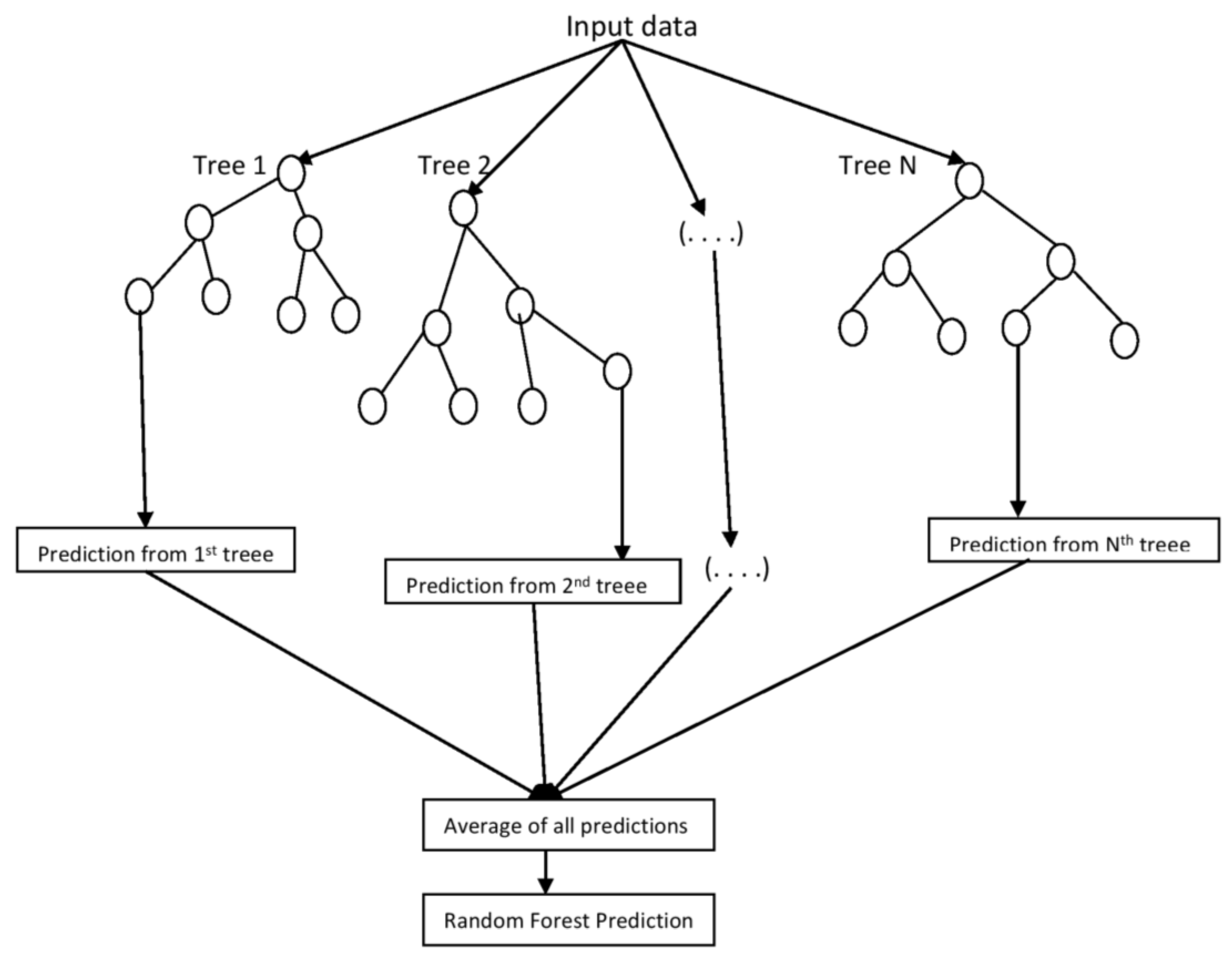Figure 1 illustrates the forest building process in the case of regression. A randomly chosen subset of the training data, which may be produced via replacement, forms each regression tree.

A specific number, $m < M$, is selected from a total of $M$ input variables. Every node is divided using the best split based on $m$ variables chosen randomly from the $M$ available variables. Starting at the root node, several approaches exist to find the best split at a node. Typically, the quality of a particular split is evaluated using the Gini Index/Cross-Entropy and the sum of squared errors ($SSE$) for classification and regression, respectively [42]. The $SSE$ for a tree $T$ is given as

$$SSE=\sum _{c\in leaves\left(T\right)}\sum _{i\in c}{(y_i-m_c)}^2$$

where $m_c=\frac{1}{n_c}\sum _{i\in c}{y}_i$ is the prediction for leaf $c$.

An input or predictor and its value in the training set that produces the lowest $SSE$ value are the basis for the first split in regression trees, and the same criteria are used to select subsequent splits. A tree can be regulated by using a stopping criterion, or grown all the way to the bottom. In general, the data may be overfit by a deep tree. Cultivating small or shallow trees is possible by applying a depth-controlling criterion. Pruning is reducing a large tree to a smaller, shallower tree. Pruning techniques were proposed by Breiman et al. [43]. These techniques include letting a tree reach its maximum size before determining whether it is overfitting the data. The overfitted tree is then reduced in size by eliminating sub-branches that don’t improve the generalization accuracy. But RF is an ensemble of these trees, so a number of trees are grown simultaneously using the aforementioned procedure of tree cultivation to build the forest. In the case of RF, pruning of trees is not required; in fact, we can decide the depth of trees just before the forest building process.

The value of $m$ remains constant while the forest is being constructed. It is possible to modify $m$ according to the dataset’s properties; however, it is usually set to the square root of the entire number of input variables in classification and one-third of the entire number of input variables in the case of regression. These default values are commonly recommended, but the optimal number can vary and should be tuned for a specific problem. In fact, if the number of inputs/predictors is low in the study, then the available number of inputs/predictors can be set equal to $m$. Low value of $m$ introduces maximum randomness into the model’s structure and ensures that the individual decision trees within the forest are as uncorrelated as possible. It helps prevent overfitting, but it may lead to higher bias, while larger values of $m$ produce more correlated trees, decreasing randomness, and may increase the variance.

A fresh training set is created by random sampling for each iteration. While building each tree, these samples are taken with replacement. A set of $n$ samples is chosen with replacement to grow each tree if the training set contains $N$ instances. Just 66% of the samples are used for training of each tree; the remaining data, called out-of-bag (OOB) data, is used to quantify error and variable importance. The OOB samples are utilized as test inputs for the relevant tree to produce predictions. Since we are dealing with a regression problem, the averaging procedure is then applied to all OOB samples across all trees. In this manner, several trees are cultivated simultaneously and trained independently using different bootstrap samples. Each tree is developed to its maximum potential, although users can also create shallower trees by adjusting the depth parameter.

RT, the base algorithm, is a nonparametric modeling technique that is relatively insensitive to outliers and quick in generating output rules, which are then used to score new datasets. However, a disadvantage of RT is its susceptibility to overfitting, particularly when the underlying data properties change. In contrast, as outlined earlier, the RF algorithm reduces overfitting through randomization and iterative processes applied to the base decision tree, leading to more stable results and better generalization on unseen data. The following sections demonstrate that the RF algorithm performs well and generalizes effectively.

Using the original training dataset, the error $e$ is first computed for the out-of-bag (OOB) data to evaluate the importance of each input variable in the prediction. A fresh set of samples is then created by randomly permuting the $p^{th}$ variable for each input variable ${ x}_p$, where $p\in \{1,\dots ,M\}$. The fresh set of samples is then used to calculate the OOB error estimate ${ e}_p$. The $p^{th}$ variable’s significance is indicated by the difference between the two errors ($e-e_p$).

The RF algorithm has three critical parameters: the number of trees to be grown, the number of predictors to be chosen at random, and the tree depth. This study explores these parameters in detail. Additionally, the importance of variables in prediction is estimated. The sum of the squared error was used as the splitting criterion.

3. Results

In this study, we aimed to create a machine learning model for coating data that delivers precise outcome predictions with minimal error. To accomplish this, we utilized the powerful RF regressor technique. This section details the implementation of RF on drying data and showcases the results, all produced using Python software (Python 3.14.0).

We have a total of 16,258 samples generated through experiments conducted under various operating conditions. Given the large size of the dataset, there is an opportunity to examine how the number of training samples affects the OOB error. Of the 16,258 samples, 75% were randomly selected for training, while the remaining 25% were reserved for testing. Initially, we investigated how the number of trees grown in the model impacts accuracy using the training samples. We created the forest for both values of $m$, i.e., $m=1$ and $m=2$, because $m$ is set to a value less than $M$. This study has only three input variables, so the default value of $m$ will be unity. In both cases, $m=1$ and $2$, the forest was found to be producing satisfactory results. In this work, all the results are demonstrated for $m=2$ only.

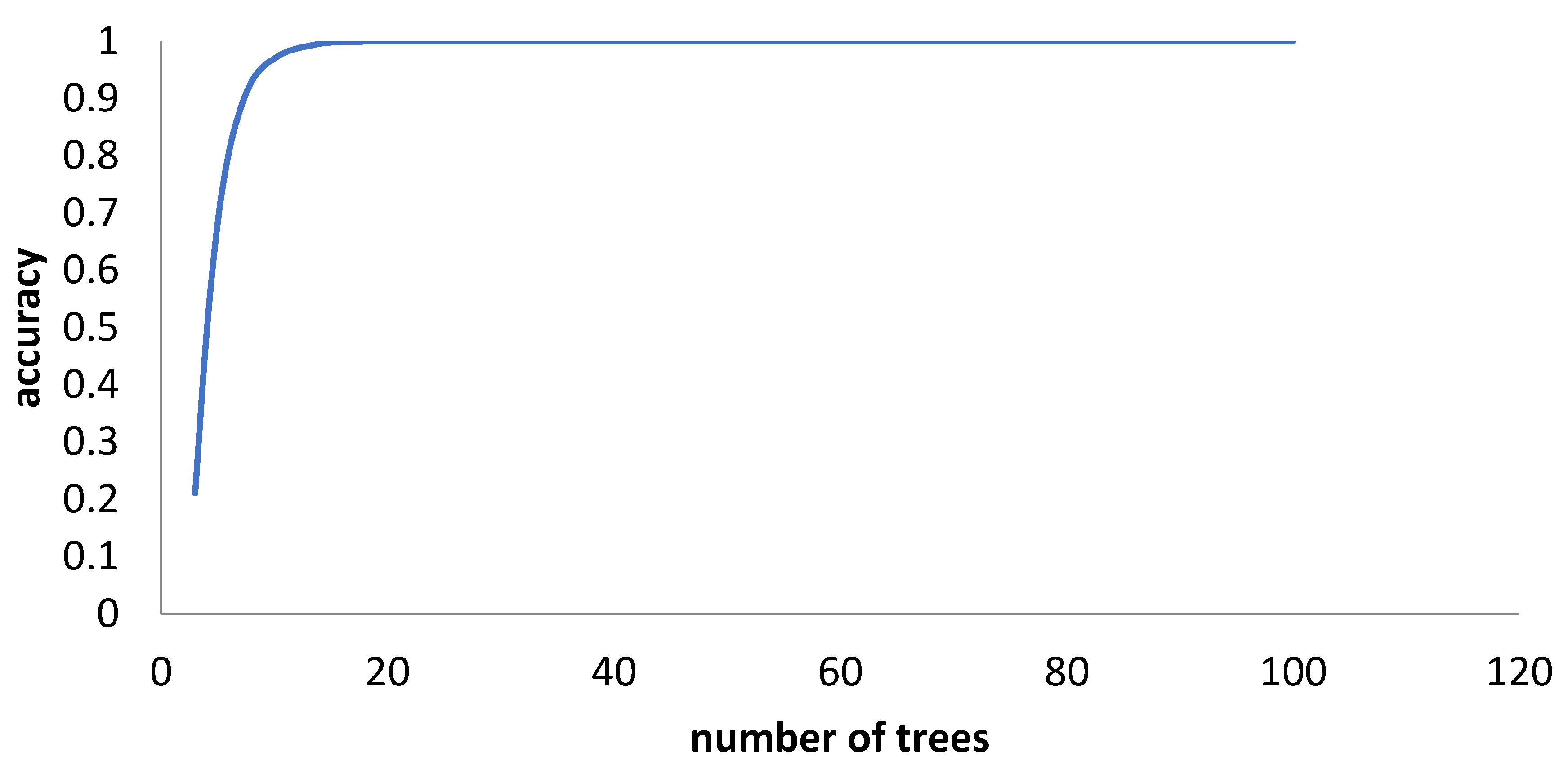
Figure 2 demonstrates that an ensemble of only twenty trees achieved 100% accuracy. We predicted the testing samples’ outputs with this ensemble of fully grown trees. The following parameters were calculated to assess the prediction accuracy:

(i) Mean squared error ($MSE$): How far the desired model’s outputs deviate from the actual value is determined by the $MSE$. A lower $MSE$ indicates that the model is functioning correctly and that there is little difference between the output that the model estimates and the actual result.

$$MSE={\displaystyle \frac{1}{n}}\sum _{i=1}^n{{(y}_i-{\mathrm{ŷ}}_i)}^2$$

$n$ = number of samples

$y_i$ = actual values

${\mathrm{ŷ}}_i$ = model’s output

(ii) Additionally, the correlation coefficient $R^2$ displays the degree of association between the estimated and calculated values; the greater its value, the closer the relationship is, and the smaller the difference between the estimated and calculated values.

$$R^2={\displaystyle \frac{\sum {{(\mathrm{ŷ}}_i-\overline{y})}^2}{\sum {(y_i-\overline{y})}^2}}$$

${\mathrm{ŷ}}_i$ = model’s output

$\overline{y}$ = mean of all values

$y_i$ = actual values

(iii) OOB error, which we have already discussed in the previous section.

All three parameters were obtained as follows:

Mean Squared Error: $9\times {10}^{-9}$

R-squared: 0.9999

OOB error: 0

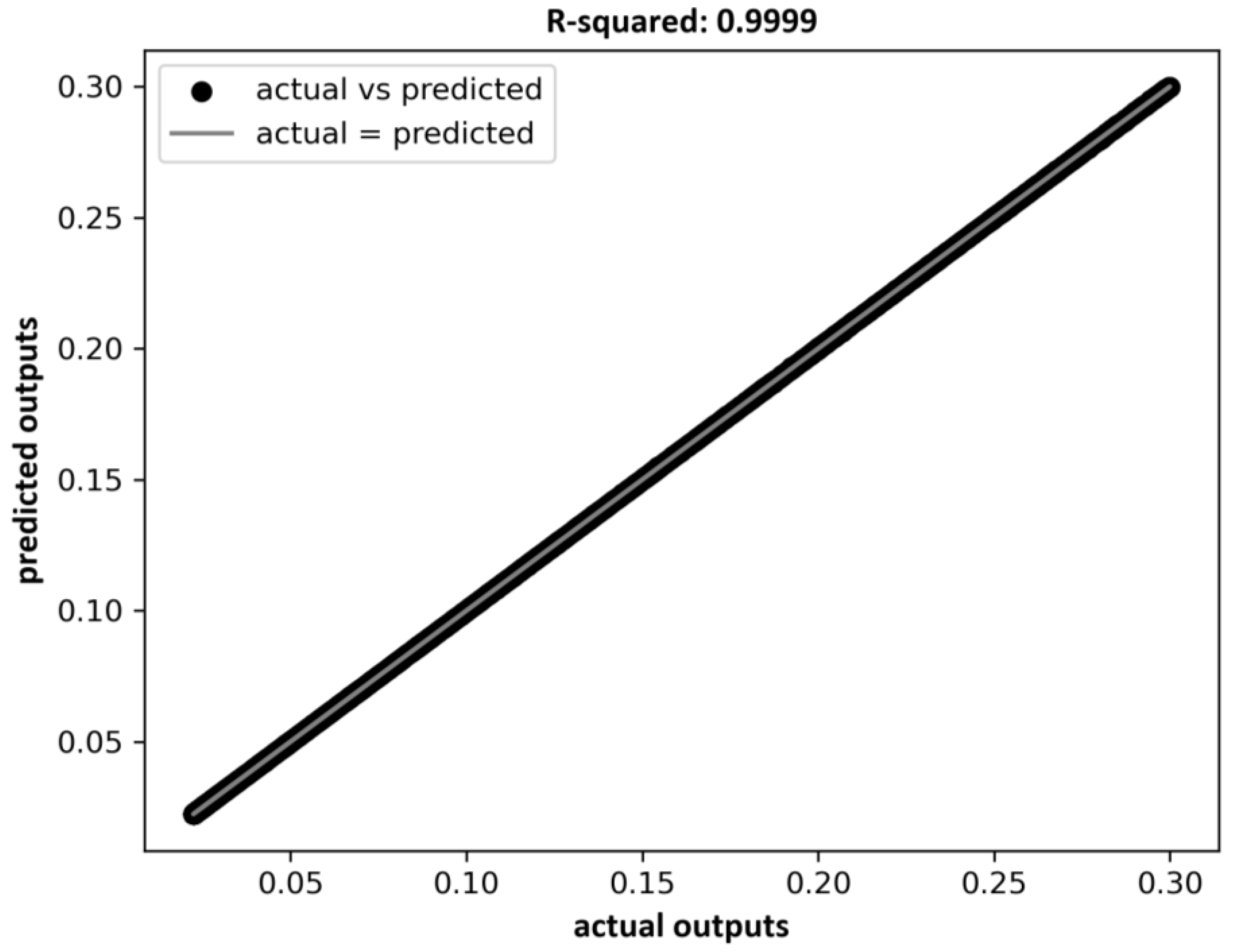
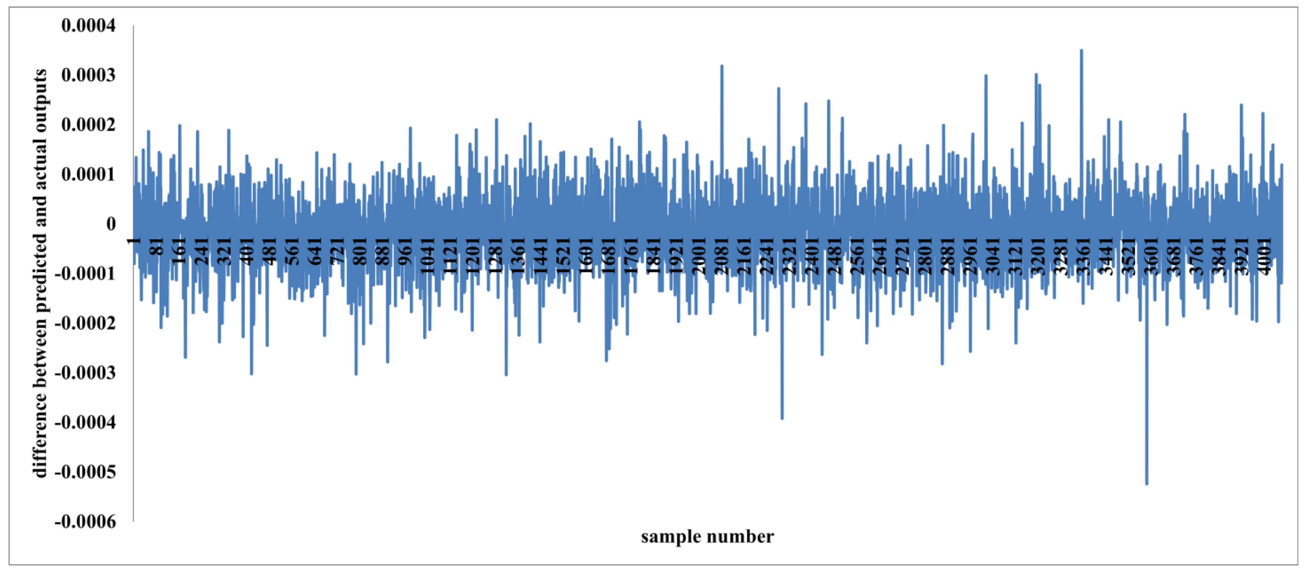
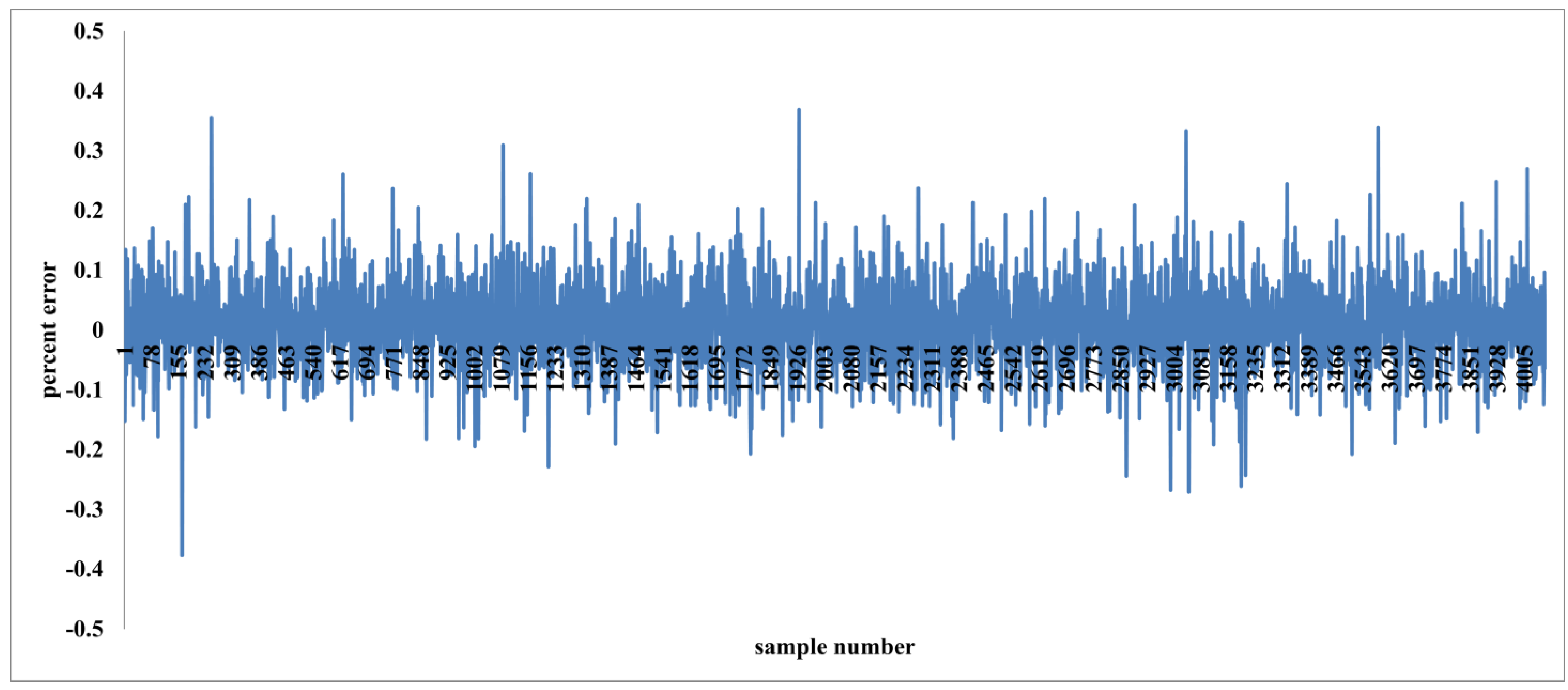
Figure 3 clearly shows that the actual outputs closely match the predicted outputs; the predicted values almost entirely overlap the actual outputs. Figure 4 displays the differences between actual and predicted outputs, which are negligible. Figure 5 presents the percent error for individual samples, revealing that the error is minimal for nearly all cases. 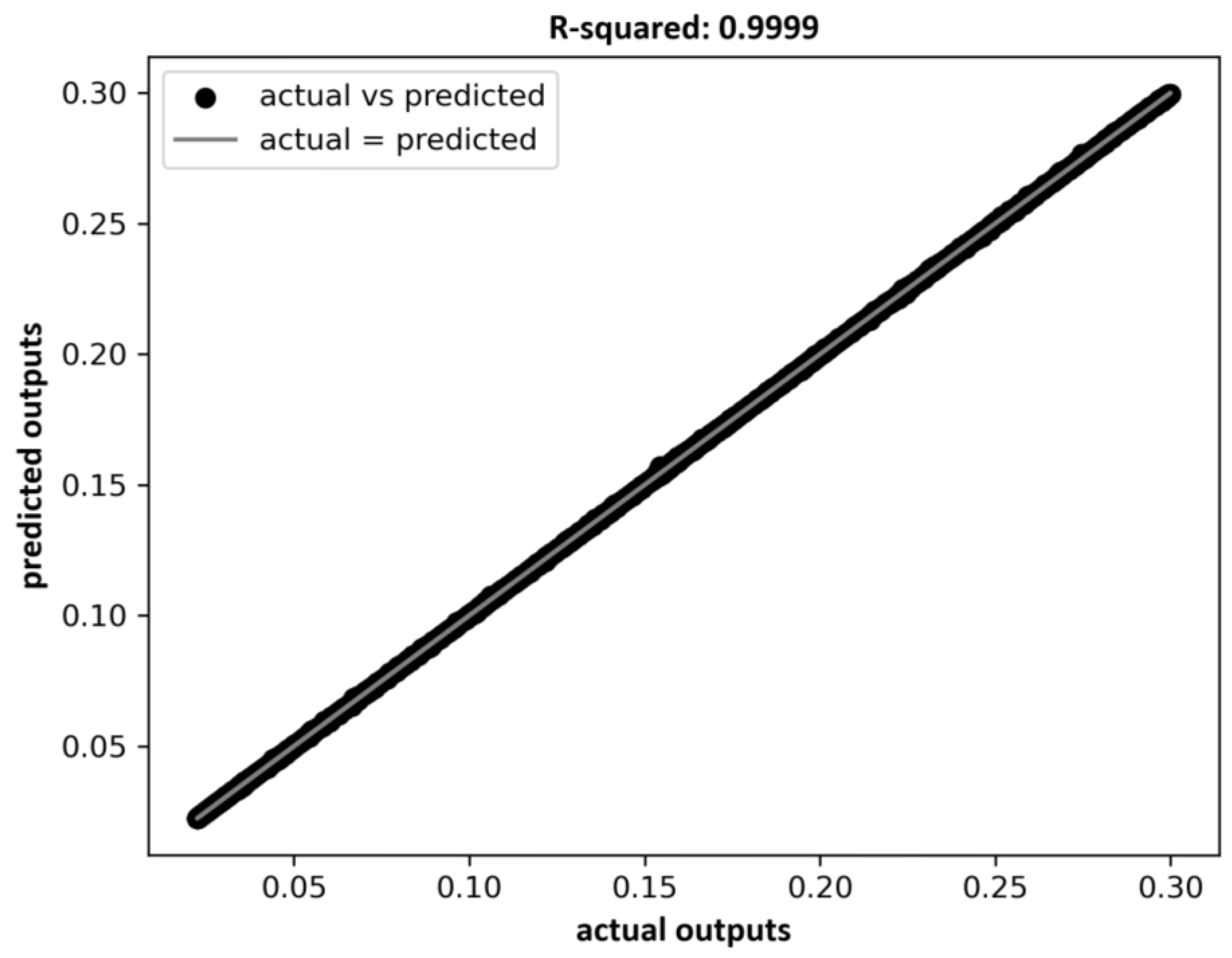This observation is further confirmed by Figure 6, where the actual versus predicted output curve perfectly overlaps the ideal equality line.

Since we have a large number of samples, we can explore how the size of the training set impacts the accuracy achieved.

Even when trained with only 20% of the data (3251 samples), this random forest model, consisting of just twenty trees, is able to predict the remaining 80% (13,007 samples) with high accuracy. This is evident from Figure 7 and Figure 8, where the percent error between actual and predicted outputs mostly falls within ±2%. The following parameters were calculated to validate this result:

Mean Squared Error: $6.7\times {10}^{-8}$

R-squared: 0.9999

OOB error: 0

Figure 7. The percent error between actual outputs and outputs predicted by the RF model trained with only 20% of the entire data.

Figure 7. The percent error between actual outputs and outputs predicted by the RF model trained with only 20% of the entire data.

Figure 8. Actual output versus output predicted by the RF model, training only 20% of the data.

Figure 8. Actual output versus output predicted by the RF model, training only 20% of the data.

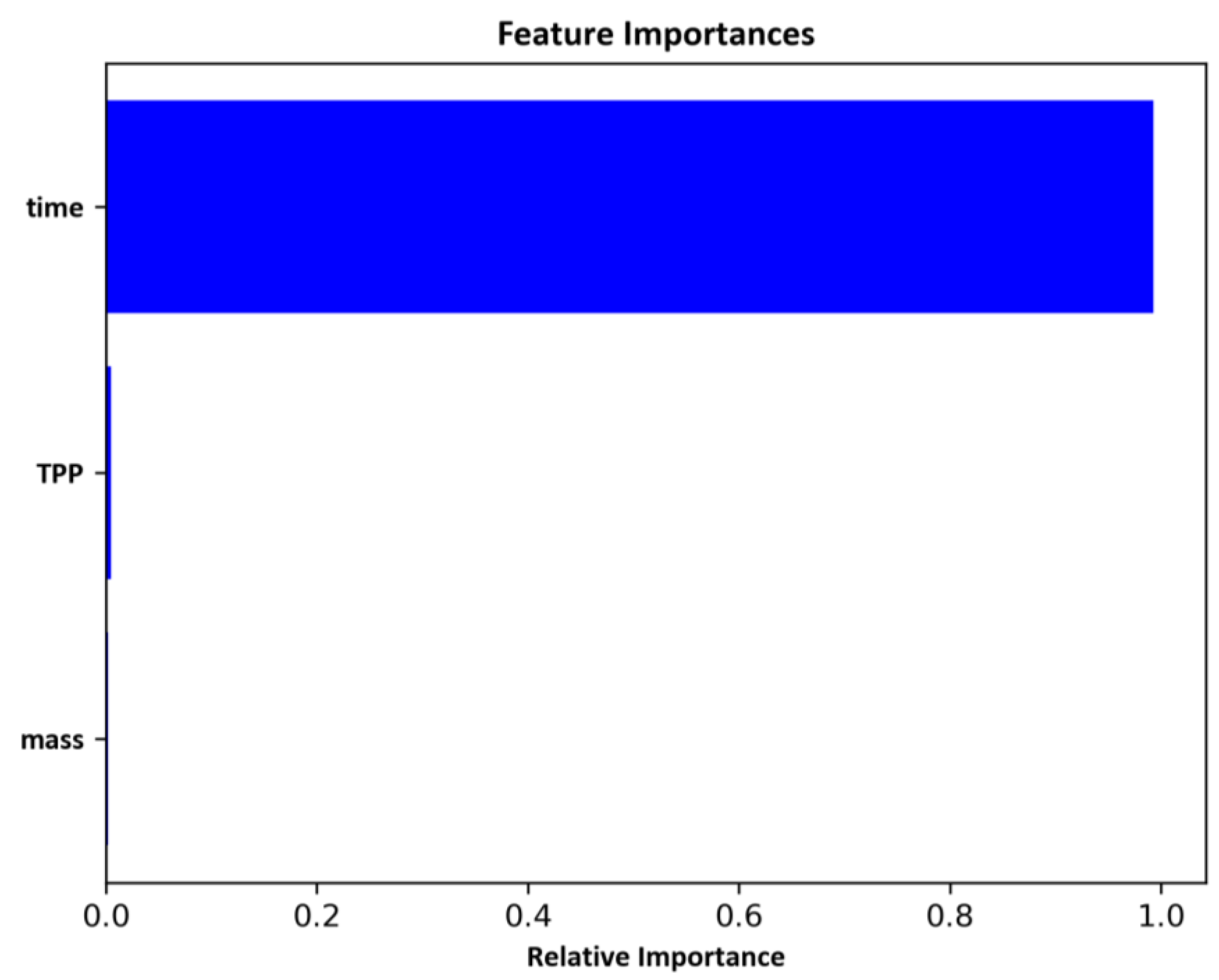
Another notable advantage of the RF regressor is its ability to assess the importance of input variables in predicting the output. Figure 9 illustrates the variable importance scores computed by the model. It is evident from the diagram that time is the most influential variable, while TPP and mass contribute minimally to the output prediction. The importance scores for each variable are as follows:

Time: 0, Score: 0.99409

Mass: 1, Score: 0.00200

TPP: 2, Score: 0.00392

Figure 9. Feature importance for input variables: $time$, $TPP$, and $mass$.

Figure 9. Feature importance for input variables: $time$, $TPP$, and $mass$.

4. Discussion

In our previous study [9], we applied a single regression tree to the same dataset. The tree-based model achieved good accuracy when trained with a large number of samples. Regression trees are generally prone to overfitting when grown to their full extent; however, we did not encounter this issue due to the availability of a large dataset. When overfitting occurs, tree pruning is typically required. Nonetheless, the model’s performance deteriorated significantly when trained with only 20% of the samples, even after pruning.

In another study [38], we applied ANN to the same dataset. A single-layer feed-forward network with back propagation was used. It was found that ANN is highly effective to model complex systems particularly when sufficient amount of data is available for training, but at the same time they have several drawbacks like computationally intensive, large number of parameters are required to tune (such as the number of hidden layers, number of neurons in the hidden layers, number of epochs, learning rate, etc.), and need cross-validation during training. Additionally, ANNs are complicated to understand. Similar to the regression tree, the performance of the ANN deteriorated when it was trained using only 20% of the available samples.

In this study, the RF model predicts unseen data with negligible error. In fact, the model trained on a relatively small subset of the data can accurately predict a much larger portion demonstrates its robustness and strong generalization capability on unseen data. Not only does our model produce negligible prediction errors, but it also generalizes well both through interpolation and extrapolation. In this case, we used deep trees (grown to their maximum depth) and allowed two variables to be considered for each node split. If the results were not satisfactory, we could have increased the model’s randomness by limiting tree depth (shallow trees) or/and tune the value of $m$, which is a standard practice in enhancing ensemble diversity.

It is evident from the results generated in this study that unlike regression tree and ANN, RF can be trained on a small subset of dataset and generalizes well the unseen data. The model trained only with 20% (3251) samples predicted the remaining 80% (13,007) samples with very high accuracy. Hence, in situations where only a limited number of samples are available, RF is a more suitable choice compared to regression trees and ANNs. In addition to its robustness against overfitting, RF is easier to interpret, requires minimal parameter tuning or pruning, and is computationally less intensive than ANN.

In addition to the aforementioned advantages, it provides an inherent ability for feature extraction. We can find out which input variables are most vital and use this information to create a simplified model that only connects the most important inputs to the output. The model’s complexity rises along with the number of input variables. Adding unnecessary or irrelevant variables might cause noise and weaken model performance. As a result, it is decisive to narrow down the feature space by choosing only the most relevant variables.

This method is beneficial when large numbers of input variables are involved. This technique also helps to determine which variables significantly influence the output; it gives insights into the system dynamics.

According to the RF algorithm’s feature importance analysis for the PSPX system, time is the most important input variable for coating weight loss prediction compared to the amount of surfactant and the initial coating thickness. This aspect of RF makes it an effective method for dimensionality reduction, which is lowering a dataset’s feature count.

The low statistical weight of TPP in the RF model arises from both experimental and mechanistic factors. In the present PSPX–TPP formulations, the concentration range of TPP (0–2 wt%) lies below the threshold typically required to induce significant alterations in polymer segmental mobility or diffusion pathways. Studies have shown that triphenyl phosphate acts as an auxiliary plasticizer at low concentrations, influencing polymer relaxation dynamics but not substantially modifying solvent diffusion rates or bulk evaporation kinetics [44,45,46]. Under these conditions, the drying behavior is predominantly controlled by solvent mass transfer, surface evaporation, and film-thickness-dependent diffusion mechanisms, all of which are strongly time-driven [47,48]. Consequently, Time emerges as the dominant predictor in the model, while TPP’s marginal quantitative variation leads to a statistically weak signal.

Furthermore, machine learning algorithms such as RF attribute feature importance based on variance and information gain. Parameters exhibiting narrow data ranges or subtle nonlinear effects are often statistically suppressed despite their physicochemical relevance [43].

5. Conclusions

In this study, RF regressor, a robust and widely used machine learning method, was applied to model the surfactant-enhanced drying behavior of PSPX coatings. TPP was added as a surfactant to accelerate solvent removal. The RF model predicts the coating’s weight loss using three input variables: drying time, TPP concentration, and initial coating thickness. The RF model trained on 80% of samples achieved prediction errors within ±0.5% on the remaining 20%, which is a testament to its accuracy. Even when trained on only 20% of the data, it still predicted the other 80% with errors within ±2%, clearly demonstrating robustness and strong generalization. RF performs well even with limited data. It combines bootstrap sampling (“bagging”) and random feature selection, which reduces variance and helps the model to generalize even with fewer samples. RF evaluates feature importance, enabling it to naturally select and prioritize key predictors—critical when handling many variables. This interpretability helps uncover system dynamics. It has Built-in resistance to overfitting. Bagging and feature randomness generate diverse trees whose errors cancel out. Unlike standalone regression trees or ANNs, RF doesn’t typically require explicit pruning or extensive cross-validation, respectively, as ensemble aggregation inherently guards against overfitting. In this work, TPP experimentally contributes to reducing residual solvent content at equilibrium, its effect is not strongly captured in the instantaneous weight-loss profiles used for model training. Future work will address this by incorporating higher TPP concentrations, in situ spectroscopic data, and explainable ML tools such as SHAP and partial dependence analyses to better resolve the chemical–statistical correlation.

References

- Arya, R.K.; Thapliyal, D.; Sharma, J.; Verros, G.D. Glassy polymers—Diffusion, sorption, ageing and applications. Coatings 2021, 11, 1049. [Google Scholar] [CrossRef]
- Kajiya, T.; Kobayashi, W.; Okuzono, T.; Doi, M. Controlling the drying and film formation processes of polymer solution droplets with addition of small amount of surfactants. J. Phys. Chem. B 2009, 113, 15460–15466. [Google Scholar] [CrossRef] [PubMed]
- Sakamoto, K.; Lochhead, R.Y.; Maibach, H.I.; Yamashita, Y. Cosmetic Science and Technology: Theoretical Principles and Applications; Elsevier: Amsterdam, The Netherlands, 2017. [Google Scholar]
- Balazs, A.C.; Hu, J.Y. Effects of surfactant concentration on polymer-surfactant interactions in dilute solutions: A computer model. Langmuir 1989, 5, 1230–1234. [Google Scholar] [CrossRef]
- Baglioni, M.; Sekine, F.H.; Ogura, T.; Chen, S.-H.; Baglioni, P. Nanostructured fluids for polymeric coatings removal: Surfactants affect the polymer glass transition temperature. J. Colloid Interface Sci. 2022, 606, 124–134. [Google Scholar] [CrossRef] [PubMed]
- Sharma, D.; Sharma, J.; Arya, R.K.; Ahuja, S.; Agnihotri, S. Surfactant enhanced drying of waterbased poly (vinyl alcohol) coatings. Prog. Org. Coat. 2018, 125, 443–452. [Google Scholar] [CrossRef]
- Sharma, I.; Sharma, J.; Ahuja, S.; Arya, R.K. Optimization of sodium dodecyl sulphate loading in poly (vinyl alcohol)-water coatings. Prog. Org. Coat. 2019, 127, 401–407. [Google Scholar] [CrossRef]
- Arya, R.K.; Kaur, H.; Rawat, M.; Sharma, J.; Chandra, A.; Ahuja, S. Influence of plasticizer (triphenyl phosphate) loading on drying of binary coatings: Poly (styrene)-p-xylene coatings. Prog. Org. Coat. 2021, 150, 106001. [Google Scholar] [CrossRef]
- Arya, R.K.; Sharma, J.; Shrivastava, R.; Thapliyal, D.; Verros, G.D. Modeling of surfactant-enhanced drying of poly (styrene)-p-xylene polymeric coatings using machine learning technique. Coatings 2021, 11, 1529. [Google Scholar] [CrossRef]
- Martin-Fabiani, I.; Lesage de la Haye, J.; Schulz, M.; Liu, Y.; Lee, M.; Duffy, B.; D’Agosto, F.; Lansalot, M.; Keddie, J.L. Enhanced water barrier properties of surfactant-free polymer films obtained by macroraft-mediated emulsion polymerization. ACS Appl. Mater. Interfaces 2018, 10, 11221–11232. [Google Scholar] [CrossRef]
- Jiang, B.; Tsavalas, J.G.; Sundberg, D.C. Water whitening of polymer films: Mechanistic studies and comparisons between water and solvent borne films. Prog. Org. Coat. 2017, 105, 56–66. [Google Scholar] [CrossRef]
- Ortona, O.; D’Errico, G.; Paduano, L.; Sartorio, R. Ionic surfactant–polymer interaction in aqueous solution. Phys. Chem. Chem. Phys. 2002, 4, 2604–2611. [Google Scholar] [CrossRef]
- Debeaufort, F.; Voilley, A. Effect of surfactants and drying rate on barrier properties of emulsified edible films. Int. J. Food Sci. Technol. 1995, 30, 183–190. [Google Scholar] [CrossRef]
- Hoff, E.; Nyström, B.; Lindman, B. Polymer−surfactant interactions in dilute mixtures of a nonionic cellulose derivative and an anionic surfactant. Langmuir 2001, 17, 28–34. [Google Scholar] [CrossRef]
- Angus-Smyth, A.; Bain, C.D.; Varga, I.; Campbell, R.A. Effects of bulk aggregation on pei–sds monolayers at the dynamic air–liquid interface: Depletion due to precipitation versus enrichment by a convection/spreading mechanism. Soft Matter 2013, 9, 6103–6117. [Google Scholar] [CrossRef]
- Nizri, G.; Lagerge, S.; Kamyshny, A.; Major, D.T.; Magdassi, S. Polymer–surfactant interactions: Binding mechanism of sodium dodecyl sulfate to poly (diallyldimethylammonium chloride). J. Colloid Interface Sci. 2008, 320, 74–81. [Google Scholar] [CrossRef] [PubMed]
- Hai, M.; Han, B. Study of interaction between sodium dodecyl sulfate and polyacrylamide by rheological and conductivity measurements. J. Chem. Eng. Data 2006, 51, 1498–1501. [Google Scholar] [CrossRef]
- Petrovic, L.B.; Sovilj, V.J.; Katona, J.M.; Milanovic, J.L. Influence of polymer–surfactant interactions on o/w emulsion properties and microcapsule formation. J. Colloid Interface Sci. 2010, 342, 333–339. [Google Scholar] [CrossRef] [PubMed]
- Talwar, S.; Scanu, L.; Raghavan, S.R.; Khan, S.A. Influence of binary surfactant mixtures on the rheology of associative polymer solutions. Langmuir 2008, 24, 7797–7802. [Google Scholar] [CrossRef] [PubMed]
- Müller, M.; Scharfer, P.; Kind, M.; Schabel, W. Influence of non-volatile additives on the diffusion of solvents in polymeric coatings. Chem. Eng. Process. Process Intensif. 2011, 50, 551–554. [Google Scholar] [CrossRef]
- Anthony, O.; Zana, R. Interactions between water-soluble polymers and surfactants: Effect of the polymer hydrophobicity. 1. Hydrophilic polyelectrolytes. Langmuir 1996, 12, 1967–1975. [Google Scholar] [CrossRef]
- Anthony, O.; Zana, R. Interactions between water-soluble polymers and surfactants: Effect of the polymer hydrophobicity. 2. Amphiphilic polyelectrolytes (polysoaps). Langmuir 1996, 12, 3590–3597. [Google Scholar] [CrossRef]
- Gu, Z.; Alexandridis, P. Drying of films formed by ordered poly (ethylene oxide)− poly (propylene oxide) block copolymer gels. Langmuir 2005, 21, 1806–1817. [Google Scholar] [CrossRef]
- Meconi, G.M.; Ballard, N.; Asua, J.M.; Zangi, R. Adsorption and desorption behavior of ionic and nonionic surfactants on polymer surfaces. Soft Matter 2016, 12, 9692–9704. [Google Scholar] [CrossRef]
- Okazaki, M.; Shioda, K.; Masuda, K.; Toei, R. Drying mechanism of coated film of polymer solution. J. Chem. Eng. Jpn. 1974, 7, 99–105. [Google Scholar] [CrossRef]
- Ravichandran, S.; Kumari, C.R.T. Effect of anionic surfactant on the thermo acoustical properties of sodium dodecyl sulphate in polyvinyl alcohol solution by ultrasonic method. J. Chem. 2011, 8, 77–84. [Google Scholar] [CrossRef]
- Ruckenstein, E.; Huber, G.; Hoffmann, H. Surfactant aggregation in the presence of polymers. Langmuir 1987, 3, 382–387. [Google Scholar] [CrossRef]
- Yamamura, M.; Mawatari, H.Y.Y.; Kage, H. Enhanced solvent drying in surfactant polymer blend coating. In Proceedings of the ISCST Symposium, Marina del Rey, CA, USA, 7–10 September 2008; pp. 114–117. [Google Scholar]
- Müller, M.; Kind, M.; Cairncross, R.; Schabel, W. Diffusion in multi-component polymeric systems: Diffusion of non-volatile species in thin films. Eur. Phys. J. Spec. Top. 2009, 166, 103–106. [Google Scholar] [CrossRef]
- Ulas, M.; Altay, O.; Gurgenc, T.; Özel, C. A new approach for prediction of the wear loss of pta surface coatings using artificial neural network and basic, kernel-based, and weighted extreme learning machine. Friction 2020, 8, 1102–1116. [Google Scholar] [CrossRef]
- Barletta, M.; Gisario, A.; Palagi, L.; Silvestri, L. Modelling the electrostatic fluidised bed (efb) coating process using support vector machines (svms). Powder Technol. 2014, 258, 85–93. [Google Scholar] [CrossRef]
- Tang, W.; Li, Y.; Yu, Y.; Wang, Z.; Xu, T.; Chen, J.; Lin, J.; Li, X. Development of models predicting biodegradation rate rating with multiple linear regression and support vector machine algorithms. Chemosphere 2020, 253, 126666. [Google Scholar] [CrossRef]
- Tušek, A.J.; Jurina, T.; Benković, M.; Valinger, D.; Belščak-Cvitanović, A.; Kljusurić, J.G. Application of multivariate regression and artificial neural network modelling for prediction of physical and chemical properties of medicinal plants aqueous extracts. J. Appl. Res. Med. Aromat. Plants 2020, 16, 100229. [Google Scholar] [CrossRef]
- Abrougui, K.; Gabsi, K.; Mercatoris, B.; Khemis, C.; Amami, R.; Chehaibi, S. Prediction of organic potato yield using tillage systems and soil properties by artificial neural network (ann) and multiple linear regressions (mlr). Soil Tillage Res. 2019, 190, 202–208. [Google Scholar] [CrossRef]
- Akbari, E.; Moradi, R.; Afroozeh, A.; Alizadeh, A.; Nilashi, M. A new approach for prediction of graphene based isfet using regression tree and neural network. Superlattices Microstruct. 2019, 130, 241–248. [Google Scholar] [CrossRef]
- De Stefano, C.; Lando, G.; Malegori, C.; Oliveri, P.; Sammartano, S. Prediction of water solubility and setschenow coefficients by tree-based regression strategies. J. Mol. Liq. 2019, 282, 401–406. [Google Scholar] [CrossRef]
- Zegler, C.H.; Renz, M.J.; Brink, G.E.; Ruark, M.D. Assessing the importance of plant, soil, and management factors affecting potential milk production on organic pastures using regression tree analysis. Agric. Syst. 2020, 180, 102776. [Google Scholar] [CrossRef]
- Thapliyal, D.; Shrivastava, R.; Verros, G.D.; Verma, S.; Arya, R.K.; Sen, P.; Prajapati, S.C.; Chahat; Gupta, A. Modeling of triphenyl phosphate surfactant enhanced drying of polystyrene/p-xylene coatings using artificial neural network. Processes 2024, 12, 260. [Google Scholar] [CrossRef]
- Breiman, L. Bagging predictors. Mach. Learn. 1996, 24, 123–140. [Google Scholar] [CrossRef]
- Breiman, L. Some infinity Theory for Predictor Ensembles; Technical Report 579; Statistics Dept. UCB: Berkeley, CA, USA, 2000. [Google Scholar]
- Breiman, L. Random forests mach. Learn 2001, 45, 5–32. [Google Scholar]
- James, G.; Witten, D.; Hastie, T.; Tibshirani, R. An Introduction to Statistical Learning: With Applications in R; Springer: Berlin/Heidelberg, Germany, 2013; Volume 103. [Google Scholar]
- Breiman, L.; Friedman, J.; Olshen, R.A.; Stone, C.J. Classification and Regression Trees; Chapman and Hall/CRC: Boca Raton, FL, USA, 2017. [Google Scholar]
- Mascia, L.; Kouparitsas, Y.; Nocita, D.; Bao, X. Antiplasticization of polymer materials: Structural aspects and effects on mechanical and diffusion-controlled properties. Polymers 2020, 12, 769. [Google Scholar] [CrossRef]
- Wypych, G. Handbook of Plasticizers; ChemTec Publishing: Toronto, ON, USA, 2004. [Google Scholar]
- DeFelice, J.; Lipson, J.E. The influence of additives on polymer matrix mobility and the glass transition. Soft Matter 2021, 17, 376–387. [Google Scholar] [CrossRef]
- Jarray, A.; Gerbaud, V.; Hemati, M. Polymer-plasticizer compatibility during coating formulation: A multi-scale investigation. Prog. Org. Coat. 2016, 101, 195–206. [Google Scholar] [CrossRef]
- Crank, J. The Mathematics of Diffusion; Oxford University Press: London, UK, 1975. [Google Scholar]