Abstract
With the increasing number of construction machinery operations near high-voltage power facilities, determining how to improve operational safety has become an urgent issue that needs to be addressed. To address safety hazards when autocranes operate near live high-voltage power lines, this study proposes a high-voltage proximity safety early warning method for autocranes. The method collects the electric field signals of high-voltage power lines in real time via an electromagnetic sensor array, calculates the azimuth angle of the live conductor using the MUSIC algorithm, and acquires the 3D point cloud data of the high-voltage power lines through high-density scanning with a LiDAR. By achieving time synchronization and coordinate registration of the electromagnetic sensor data and LiDAR data, a 3D spatial model of the high-voltage power lines is established, and the minimum distance between the crane boom and the live conductor is calculated. It identifies the voltage level, computes the basic safety distance, modifies the distance with environmental factors, and then multiplies it by a safety factor to obtain the dynamic safety threshold. Finally, based on the real-time distance between the crane boom and the live conductor, hierarchical early warnings and control actions are triggered.
1. Introduction
With the continuous advancement of urbanization and the increasing development of infrastructure construction in China, the operating environment at construction sites has become more complex, particularly in construction areas surrounding high-voltage transmission lines [1,2]. As a core piece of large-scale construction machinery, autocranes are widely used in various fields such as high-rise building construction, bridge construction, and the installation of large-scale facilities, owing to their advantages of strong mobility, wide operating range, and high adaptability [3]. However, in these complex construction environments, metal components of cranes—such as booms and slings—often inadvertently intrude into the safety zone of high-voltage power facilities due to operational errors or inaccurate spatial judgment, thereby triggering serious safety accidents [4,5].
When an autocrane operates in the vicinity of energized power lines, if its boom or other components come into contact with or are excessively close to the high-voltage power lines, it may not only result in damage to expensive equipment but also severely disrupt the construction schedule [6]. More critically, damage to power equipment or accidents may lead to catastrophic consequences such as fires, arc discharges, insulation breakdown of equipment, and even electric shock casualties among workers—posing a significant threat to the stable operation of the power grid and the personal safety of personnel [7,8]. Therefore, determining how to enhance the safety of autocrane operations, particularly when working near high-voltage power facilities, has become a critical technical challenge that urgently needs to be addressed.
At present, research on proximity detection of energized electrical equipment at home and abroad mainly falls into two categories. One category involves detection through the installation of various sensors, and the other category relies on detecting the electric field intensity around high-voltage power lines. Luo et al. [9] studied the simulation calculation method for the safe distance between a crane boom and high-voltage power lines based on electric field intensity. By simplifying the high-voltage power line model and adopting the charge simulation method, an electric field intensity distribution model was constructed to analyze the safe distance between the crane boom and the high-voltage power lines. The research results show that the electric field intensity around the high-voltage power lines is basically the same at equal distances, and the presence of the crane has a certain impact on the electric field intensity. By establishing a linear correction relationship between the electric field intensity and the crane, a safety early warning method based on electric field intensity detection was proposed. Experimental results verify the effectiveness of the proposed model and method, which can accurately estimate the electric field changes when the boom approaches the high-voltage power lines, thereby effectively avoiding electric shock accidents and improving the safety of lifting operations. Yang et al. [10] proposed an online anti-collision monitoring method for transmission lines based on cloud-fog collaborative computing. Via the camera module and microwave ranging module, moving targets are automatically detected, and the three-dimensional feature values of the identified targets—including H-histogram, minimum bounding rectangle of the sample, and microwave ranging results—are collected using the fog computing method. These collected feature values are uploaded to the cloud, where they are used for database construction and neural network training. The particle swarm optimization algorithm is employed to optimize the initial values of the neural network. When a foreign object approaches the lines again, the results of cloud-fog collaborative computing can be utilized to determine whether the object is a threatening sample and issue an early warning in a timely manner. Experimental results demonstrate that the recognition accuracy of the proposed method can reach 95.97%, enabling it to provide reliable monitoring results.
Although existing research has made certain progress in the field of high-voltage proximity detection, there are still three key research gaps: First, the limitations of single-sensor technology are significant. Traditional electromagnetic sensors are vulnerable to interference from complex electromagnetic environments, resulting in large ranging accuracy errors; ultrasonic sensors are affected by temperature, humidity, and air flow, leading to a high false alarm rate under rainy and foggy working conditions; although a single LiDAR offers high accuracy, it has problems such as blind spots in field coverage and target confusion in scenarios with multiple high-voltage lines, making it difficult to independently meet the needs of dynamic operations [11]. Second, the adaptability of multi-sensor fusion research is insufficient. Although the existing cloud-fog collaborative vision + microwave fusion method has improved recognition accuracy, it focuses on static foreign object detection of transmission lines and does not design synchronization and registration mechanisms for the dynamic operation characteristics of automatic cranes, failing to meet the real-time requirements of construction. Third, the safety threshold model lacks dynamic adaptability. Most existing methods adopt fixed safety distance thresholds and do not comprehensively consider the impact of environmental factors and hoisting conditions on the safety distance, which leads to a decline in early warning accuracy under complex working conditions [12].
To address the aforementioned issues, this study introduces three innovative improvements to advance existing work: First, it establishes a dual-sensor fusion framework. An electromagnetic sensor array is used to collect electric field signals in real time, and the MUSIC algorithm is applied to calculate the azimuth angle of high-voltage lines. This guides the LiDAR to perform directional high-density scanning, thereby resolving the problem of insufficient field-of-view coverage of LiDAR. Second, it designs a coordination mechanism adapted to dynamic operations. The ICP coordinate registration algorithm is employed to achieve synchronization between the data from the electromagnetic sensor and the LiDAR, meeting the requirements of dynamic boom operations. Third, it develops a multi-factor dynamic safety threshold model. By integrating high-voltage level identification, environmental factor correction, and operational safety coefficients, this model overcomes the limitations of traditional fixed thresholds.
This method specifically fills the technical gap in high-voltage proximity early warning for dynamic operation scenarios and provides a more optimized solution for safety monitoring of automatic cranes under complex working conditions.
Against the backdrop of advancing China’s “carbon neutrality” goal, the processes of energy transition and green infrastructure construction (such as large-scale wind power, photovoltaic power transmission projects, and smart grid upgrades) have accelerated significantly. The implementation of such green projects relies heavily on crane operations, which has greatly increased the frequency of close-range interaction between cranes and high-voltage lines. Ensuring the operational safety of cranes near high-voltage lines is not only a basic requirement for protecting personnel and equipment, but also a key support for the steady advancement of green infrastructure [13,14]. Therefore, the research and development of this study not only holds practical significance but also provides technical support and practical experience for the application of similar technologies in a broader range of engineering fields in the future.
2. Critical Technologies
For boom proximity detection, electromagnetic sensors are usually installed to monitor changes in the external magnetic field so as to estimate the distance to live electrical equipment and achieve an early warning function. However, this method has insufficient measurement accuracy and cannot meet the requirements of precision operations. Ultrasonic technology is also commonly used for proximity detection, but it is susceptible to environmental interference, resulting in low reliability of measurement results.
This study proposes a high-voltage proximity safety early warning method based on the data fusion of electromagnetic sensors and LiDAR. By integrating the LiDAR with the boom, the working status of the autocrane’s boom is monitored in real time through operations such as shape scanning, point cloud processing, and spatial straight-line distance calculation. This enables operators to obtain more intuitive and accurate information, effectively ensuring the safety of personnel and equipment.
2.1. LiDAR
LiDAR (Light Detection and Ranging) features a wide detection range, high resolution, and high accuracy [15,16]. It is convenient to install and is not affected by the telescopic state of the boom. Its measurement values are accurate, and it can monitor the changes in the deflection of the autocrane’s boom in real time, which can provide guarantees for the safety of crane operations. Therefore, LiDAR is used to detect the boom deflection through visual perception technology. The physical object of the LiDAR device is shown in Figure 1, and the main parameters are detailed in Table 1.
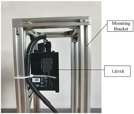
Figure 1.
Livox HAP LiDAR.

Table 1.
Parameters of Livox HAP LiDAR.
2.2. Point Cloud Data
Three-dimensional (3D) point cloud data consists of a large number of points with attributes such as 3D position, laser echo intensity, and color, and is capable of representing spatial information. By scanning the crane boom with LiDAR, a 3D structural model of the boom can be constructed, facilitating identification and analysis [17,18]. Specifically, the distance coordinates of the point cloud are acquired via LiDAR, and these coordinates are combined with the 3D data obtained from the scanning system to form a point cloud map. This process enables the acquisition of the 3D information of the object, resulting in discrete spatial point data that reflects the structural details of the scene and the surface information of the object.
The point cloud data generated by LiDAR possesses several distinctive characteristics: (1) Point cloud data can record a series of spatial coordinate points on the surface of an object. (2) Owing to its direct representation of position information, point cloud data has obvious advantages in extracting spatial features. (3) Point cloud data can display the relative positions between different targets in three-dimensional (3D) space, and the data is presented as discontinuous, scattered points. (4) Different LiDAR systems adopt unique scanning technologies, and the scanning effect varies depending on the differences in the reflectivity of the target materials.
2.3. Point Cloud Cropping and Point Cloud Filtering
Although point cloud data covers a relatively large area, it is mainly concentrated in the central part. As the distance increases, the point cloud density gradually decreases, and the contained information decreases accordingly. Meanwhile, the figure also shows several abnormally scattered points, which are noise points. After LiDAR scans the data, noise points may be generated due to the following three situations: (1) system errors—each system may introduce noise points; (2) noise points caused by objects with special materials; (3) external interference during scanning, which leads to errors and the formation of noise points. Noise points are useless points that can interfere with effective information. To improve data quality and processing efficiency, it is necessary to eliminate point cloud data in non-focus areas and retain only the point set that can provide useful information. Sometimes, it is also necessary to remove certain points inside the target area, which requires the application of point cloud cropping and filtering technologies to screen data, highlight useful information, and optimize the calculation process.
Point cloud cropping is crucial for improving the accuracy and speed of target detection, and its implementation method is simple: set the boundary values of the point cloud in three dimensions, and then compare the coordinates of each point to determine whether it is included [19].
In unprocessed LiDAR point clouds, there exist invalid data such as random points and isolated points. These invalid data may be caused by environmental factors, target characteristics, or poor sensor accuracy, thereby affecting data accuracy. To maintain data quality, such invalid data must be removed; therefore, filtering technology is adopted to process subsequent data. To improve computational efficiency, point cloud filtering is performed first, followed by point cloud cropping to eliminate non-target points. Point cloud filtering not only removes noise points and abnormal points but also has additional functions of data smoothing and data compression, which helps express point cloud information in a clearer and more concise manner. Common filtering methods include histogram filtering, voxel filtering, statistical filtering, conditional filtering, and radius filtering. In this paper, statistical filtering is selected for denoising the point cloud data.
The basic principle of statistical filtering is to calculate the average distance between each point in the point cloud and its nearest neighboring points, assuming that these average distances follow a Gaussian distribution. Outliers that are far from most points are identified and removed based on the statistical characteristics of these average distances [20,21]. Figure 2 shows a schematic diagram of point cloud statistical filtering. The average distance within the four neighboring areas of a point is represented by the black circle, and the calculated threshold is represented by the green circle. Both points a and c are valid point clouds, while point b, which exceeds the threshold distance, is regarded as an outlier and thus removed.
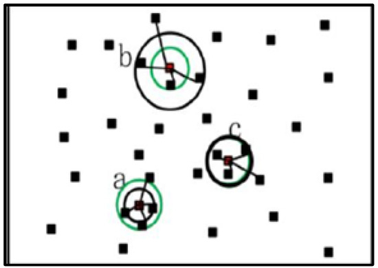
Figure 2.
Schematic Diagram of Point Cloud Statistical Filtering.
Specifically, statistical filtering calculates the average distance from each point to its nearest neighbors. This distance distribution generally conforms to a Gaussian distribution, and the mean distance and standard deviation are calculated based on the characteristics of the Gaussian distribution. Next, a threshold value is set , which is usually taken as the mean distance plus or minus times the standard deviation , i.e., . Under this threshold, if the average distance from a point to its neighboring points is higher than the threshold, the point is regarded as an outlier and removed from the point cloud. The steps of the statistical filtering algorithm are as follows [22]:
Neighborhood definition: Before performing statistical filtering, it is necessary to define the neighborhood range for each point. This neighborhood is usually composed of a specified fixed radius or a fixed number of nearest neighboring points.
Calculation of statistical information: For the point set within each neighborhood, calculate various statistical measures such as mean, variance, and standard deviation. Equations (1) and (2) are used to compute the mean and standard deviation , respectively.
(1) Noise point judgment: Based on the obtained statistical information, a certain threshold or condition is used to determine whether each point is a noise point.
(2) Filtering implementation: Once outliers are identified, these points can be removed from the point cloud, thereby obtaining the filtered point cloud data.
Figure 3 shows the flowchart of the statistical filtering algorithm.
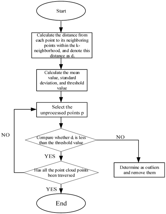
Figure 3.
Flow Chart of Statistical Filtering Algorithm.
3. Main Technological Innovations
We collect the electric field signals radiated by high-voltage lines in real time through an electromagnetic sensor array, and infer the distance based on the electric field intensity attenuation model. The electric field intensity attenuation model is as follows:
Among them, represents the measured electric field intensity using the electromagnetic sensor array, is the dielectric constant with a value of , denotes the identified voltage level of the high-voltage line, stands for the straight-line distance between the sensor and the live conductor, is the environmental attenuation factor with a value of 1.3, indicates the propagation path length of electromagnetic waves in the medium, and represents the angle between the line connecting the LiDAR and the live conductor and the horizontal plane.
The MUSIC (Multiple Signal Classification) algorithm is used to perform eigenvalue decomposition on the covariance matrix of the electric field signals received by the electromagnetic sensor array. The first K largest eigenvalues form the signal subspace, while the remaining eigenvalues form the noise subspace. The spatial spectrum function is then utilized to search for the azimuth angle of the live conductor:
In the above equation, is the array steering vector, is the azimuth angle of the live conductor, is the spatial spectrum function in the MUSIC (Multiple Signal Classification) algorithm, is the noise subspace, is the conjugate transpose of the noise subspace matrix, and is the conjugate transpose of the array steering vector.
According to the azimuth angle of the live conductor, the LiDAR is controlled to perform high-density scanning within a set angle so as to obtain the 3D point cloud data of the high-voltage line. The point cloud data of the boom, the head of each boom section, the hook’s fixed pulley block and the lifting line are acquired through point cloud processing methods including filtering, cropping and clustering. When there are nearby high-voltage lines, the LiDAR also obtains the point cloud data of these nearby high-voltage lines.
Based on the point cloud data of the first section of the boom and the protruding parts of each boom section head, the center points of each boom section and the fixed pulley block are determined. The center line position of the boom is identified using the point cloud line fitting algorithm; similarly, the center line position of the lifting line is determined according to the point cloud data of the lifting line, and the center line position of the high-voltage line is obtained from the point cloud data of the high-voltage line.
Subsequently, three sets of distances are calculated, respectively: the distance between the center point at the top of the boom and the center line of the high-voltage line, the distance between the center line of the boom and the center line of the high-voltage line, and the distance between the center line of the lifting line and the center line of the high-voltage line. These distances are then compared, and the shortest one is output as the minimum approach distance of the autocrane’s boom to the live high-voltage line. Figure 4 shows the point cloud map for detecting the approach distance of the autocrane to live high-voltage lines.
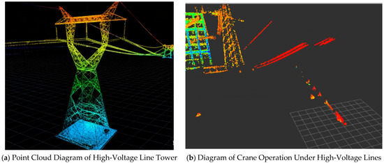
Figure 4.
Point Cloud Diagram of Proximity Distance Test for autocrane.
Among them, the explanation for the calculation of the three groups of distances is as follows:
In three-dimensional space, the distance from a point to a line can be calculated using the vector method. The following general steps are used to solve the distance from a point to a line via vectors:
- (1)
- Defining a Straight Line: Identify two points on the line, such as A (,,) and B (, , ). During the operation of the boom, the point cloud map scanned by LiDAR is processed through clipping, filtering, clustering, and other procedures. After that, the center points of the end of each boom section, the fixed pulley block, the center point of the hook, and the two endpoints of the high-voltage line are calculated. The center line of the main boom can be determined and fitted into a straight line using the center point of the end of the first boom section and the center point of the top pulley block. The high-voltage line can be fitted into a straight line via its two endpoints, while the hoisting line can be fitted into a straight line through the center point of the hook and the center point of the top pulley block.
- (2)
- Calculating the Line Vector: Calculate the direction vector of the line, which is obtained by subtracting the coordinate vector of point A from that of point B, resulting in (, , ). The direction vector can be derived from the coordinates of the two endpoints of the high-voltage line, and the equation of the line can then be expressed as
- (3)
- Obtaining Point C: Identify the target point C (, , ) in space, which is the point for which the distance is to be calculated. The coordinates of the foot of the perpendicular from point C to the line are D (, , ). Through point cloud processing, the center point of the top pulley block can be obtained, and this point represents the spatial position of the top end of the main boom.
- (4)
- Calculating Vector AD: Subtract the coordinate vector of point A from that of point D to obtain vector AD.
- (5)
- Given that the dot product of the direction vector of the perpendicular (,,) and the direction vector of the line (,, ) is zero, it can be derived thatIt can be derived from Equations (8) and (9) thatThe distance from point C to the line can be calculated as follows:
By integrating and substituting Equations (8) and (10) into Equation (11), the value of d can be calculated. Figure 5 below is a schematic diagram of the distance from a point to a line.
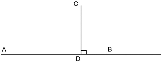
Figure 5.
Schematic diagram of distance.
From this, the distance between the top of the main boom and the high-voltage line can be obtained. During the operation of the truck crane, high-voltage lines are widely distributed, and the main boom may pass between two high-voltage lines. Moreover, wire collision accidents may occur when the boom is lifted or lowered. Therefore, it is also necessary to separately calculate the distances between the boom, the hoisting line, and the high-voltage lines.
The distance between two lines in space refers to the shortest distance between two non-intersecting lines, i.e., the perpendicular distance between the lines. The perpendicular distance can be calculated using the dot product of vectors. Specifically, the two lines can first be expressed in vector form, and then the dot product between these vectors is computed. If the angle between the two lines is 90 degrees, the distance between the two lines is equal to the product of the magnitudes of the two vectors divided by the dot product of the vectors.
Suppose there are two lines, and , whose equations are, respectively, as follows:
In Equations (12) and (13), , , , , , represent the components of the direction vector of the line; and represent the intercepts of the line. The equations of these two lines can be expressed in vector form as:
In Equations (14) and (15), take any two points ( and ) on each of the two lines, respectively. and represent direction vectors, while and represent parameters. The distance formula between these two lines can be derived by calculating their shortest distance. Suppose is a point on and is a point on ; the distance between them is , and the distance vector from to is
In Equation (16), represents the component of the direction vector along , and represents the component of the direction vector perpendicular to . Since is perpendicular to , it is also perpendicular to ; therefore, can be expressed as
Since lies on , it can be expressed as
Substituting Equation (18) into Equation (17), we get
Since is perpendicular to , the dot product of , , and the direction vector is 0, and it can be derived that
Substituting the equation of into Equation (20), we obtain
In Equation (21), represents the dot product of vectors and . The above is the method for calculating the distance between two lines in space. The process is as follows: first, calculate the cross product of the direction vectors of the two lines; then, calculate the dot product between the lines; finally, divide the result by the magnitude of the direction vector to obtain the distance between the two lines.
Time synchronization and coordinate registration are performed on the data from the electromagnetic sensor array and LiDAR. The timestamps of the electromagnetic sensor array data and multi-beam LiDAR data are aligned through linear interpolation; the ICP (Iterative Closest Point) registration algorithm is adopted to unify the electromagnetic positioning points and laser point cloud into the coordinate system with the boom root as the origin; A transformation matrix is used to unify the coordinate systems of the electromagnetic sensor array data and LiDAR data into the coordinate system with the boom root as the origin. The point cloud offset caused by boom rotation is eliminated according to a correction formula, which is as follows:
Among them, represents the corrected point cloud coordinates, is the rotation correction matrix, denotes the originally collected point cloud coordinates, stands for the linear velocity of the boom’s movement, is the time interval for LiDAR to complete the collection of one frame of point cloud, and represents the angular velocity of the boom’s movement.
Minimize the sum of squared Euclidean distances between the electromagnetic positioning points in the electromagnetic sensor array data and the laser point cloud in the LiDAR data:
Among them, is the rotation matrix, is the translation vector, is the electromagnetic positioning point, is the laser point cloud point, and is the total number of matching pairs between electromagnetic positioning points and laser point cloud points involved in registration.
Set a safety threshold for the approach distance to live high-voltage lines. When the minimum approach distance exceeds this safety threshold, an alarm signal is triggered to promptly remind staff to stop lifting operations. The calculation method for the adaptive threshold is as follows:
Among them, , , , and are compensation coefficients, with values of 0.0021, 0.015, 0.032, and 0.8, respectively; is the dust concentration output by the environmental perception module; is the voltage level; is the deviation between the ambient temperature and the standard temperature; is the relative humidity; is the environmental attenuation factor; and is the dynamic safety factor.
The flow diagram for approach distance detection to live high-voltage lines is illustrated in Figure 6.
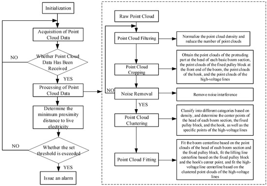
Figure 6.
Flow Chart of Proximity Detection to Live Electricity.
Based on the dynamically calculated adaptive threshold in real time, the system triggers a hierarchical early warning and executes control actions such as speed limitation, deceleration, or emergency braking, as shown in Table 2, to ensure the safety of boom operations.
Table 2.
Overview of Hierarchical Early Warning.
4. Prototype Experimental Testing and Iterative Optimization
We conducted tests at multiple actual construction sites, including urban dense areas and extreme weather conditions (such as rain, fog, etc.), to verify the stability and accuracy of the system in complex environments. The test site is illustrated in Figure 7.
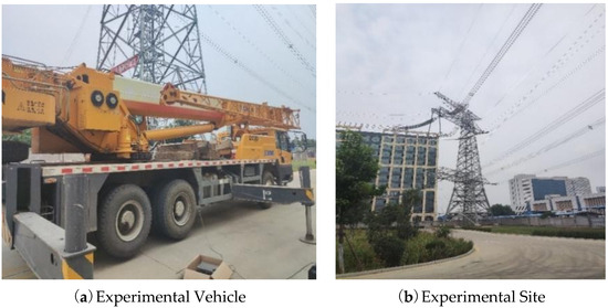
Figure 7.
Prototype Test Diagram.
To verify the reliability of the researched key technologies for the working condition safety monitoring of autocrane in real scenarios, we built a working condition safety monitoring platform based on the QY25K5C_1 crane. The monitoring platform adopts a cloud-edge-terminal integrated architecture in its implementation. For the transmission of on-site sensing data, a wireless local area network based on Long-Range Radio (LoRa) technology is used, which includes an acquisition host and acquisition terminals. The acquisition host communicates with the acquisition terminals via the LoRa network; equipped with 4G and 5G modules, the acquisition host uploads data to the cloud platform through the mobile public network (APN). The platform management host is used for platform information maintenance, as illustrated in Figure 8.
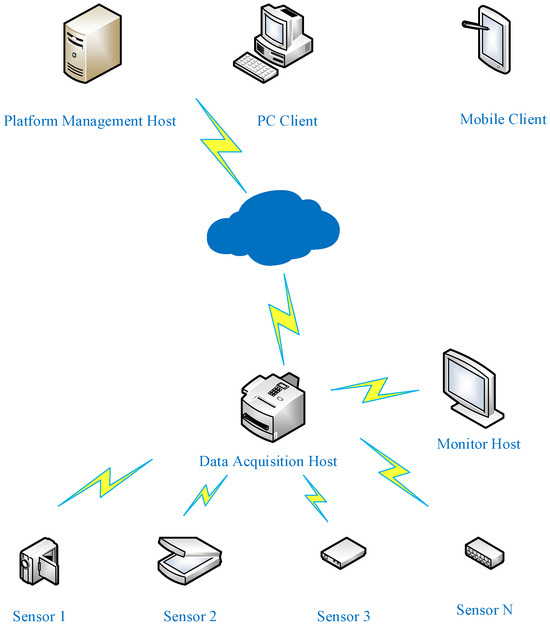
Figure 8.
Network Structure Diagram of the Monitoring Platform.
The system configuration of the built autocrane working condition safety monitoring platform is shown in Table 3.
Table 3.
System Configuration.
To facilitate communication between various modules of the intelligent monitoring platform, the experiment adopts the multi-functional distributed architecture ROS (Robot Operating System) for implementation. ROS exhibits excellent compatibility with the Ubuntu system running on the Linux kernel, which greatly simplifies the experimental operations. The software environment for the experiment in this paper is based on the Ubuntu 18.04 system, on which the corresponding ROS Melodic version is installed; meanwhile, the ROS operating environment is configured. The specific configuration of the experimental environment is shown in Table 4.
Table 4.
Specific Configuration of the Experimental Environment.
Figure 9 shows the working condition safety monitoring system for the autocrane, which integrates the status information of the autocrane during operation into a single interface to enable intuitive visualization of the crane’s safety status and prevent potential hazards; the monitoring interface is divided into 6 regions for displaying different types of information, as illustrated in Figure 10, where Region 1 displays the basic model of the autocrane, Region 2 shows the basic information and data of the crane (including the extended length of the boom, boom elevation angle, lifted weight, and hook torque), Region 3 serves as the early warning region, Region 4 is the real-time detection region for boom deflection, Region 5 is the real-time detection region for the proximity distance between the boom and live high-voltage lines, and Region 6 is the detection region for the tilt angle variation of the autocrane.
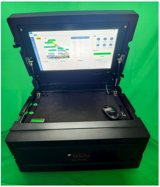
Figure 9.
Safety Monitoring System Platform for autocrane Working Conditions.
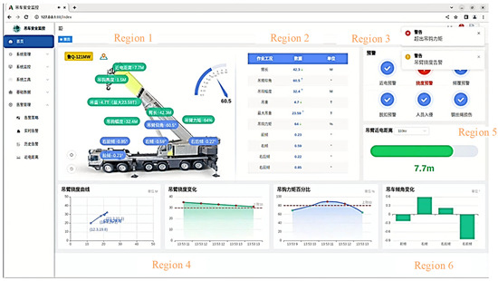
Figure 10.
Real-Time Processing Interface of the Monitoring Platform.
A boom proximity detection experiment to live high-voltage lines was conducted, where the LiDAR was fixed on the first section of the crane’s boom. The experiment was carried out on-site near high-voltage transmission lines with electric field intensities of 10 kV, 220 kV, and 500 kV, respectively. Professional personnel operated the crane’s boom to slowly approach the test high-voltage lines, with the early warning distances set as follows: 3 m for 10 kV, 5 m for 220 kV, and 8.5 m for 500 kV. When the distance between the end of the boom and the high-voltage line was less than the set threshold, an alarm was triggered. The LiDAR was used to conduct 20 experiments at each early warning distance; due to factors such as the lines being at high altitude and inaccessible for contact, the actual proximity distance in the experiment was determined based on the extended length of the autocrane’s boom, the boom’s elevation angle, and the distance of the high-voltage lines from the ground. The comparison results between the detected early warning distances and the actually calculated distances, as well as the detection errors, are shown in Table 5.
Table 5.
Experimental Data of Proximity Distance to Live Electricity.
Field experiments show that the experimental result error in the safety monitoring of proximity detection to live high-voltage lines is within 5%. Regardless of whether the high-voltage line is in front of or to the side of the boom, the measured distance and orientation are basically accurate. When the proximity distance is less than the threshold, an alarm is triggered, and the experimental results are consistent with the theoretical situation.
5. Conclusions
This study proposes a high-voltage proximity safety early warning method for autocrane based on the data fusion of electromagnetic sensors and LiDAR, which successfully addresses the issues of measurement deviation and insufficient reliability existing in traditional single-sensor technology under complex environments. By collecting the electric field signals radiated by high-voltage lines in real time and calculating the azimuth angle of live electrical equipment using the MUSIC algorithm, the system can accurately control the LiDAR to perform high-density scanning based on the azimuth angle of the high-voltage live electrical equipment, acquire the 3D point cloud data of the live electrical equipment, and thereby generate an accurate 3D model. This model provides precise data support for calculating the real-time safe distance between the crane boom and the high-voltage live electrical equipment.
Through the identification of voltage levels and dynamic correction of environmental factors, combined with safety factors, the adaptive threshold calculation method proposed in this paper effectively improves the adaptability and accuracy of the system. The real-time adjustment based on different voltage levels and environmental factors ensures the accurate calculation of the safe distance; furthermore, according to the adaptive threshold and the distance between the boom and the live electrical equipment, hierarchical early warnings and control actions are triggered, which guarantees the provision of efficient and reliable early warning information under different operating environments.
This study provides an innovative safety early warning solution for the high-voltage proximity operations of autocranes, which possess high practicality and promotion value. Especially in hoisting operations near high-voltage power facilities, it can provide more accurate and timely safety guarantees for operators, reduce safety accidents caused by proximity to live electricity or line contact, and improve the safety during the operation process.
However, despite the good performance of the system in experiments, there is still room for further optimization. For instance, the system’s real-time response capability under dynamic position changes in high-voltage lines and extreme environments can be optimized through the integration of more sensors and the adoption of more complex algorithm models. In addition, in the future, by further enhancing the computing capability of hardware devices and accelerating data processing speed, the real-time performance and adaptability of the system can be further improved, enabling it to play a role in a wider range of engineering applications.
In summary, the high-voltage proximity safety early warning method and system proposed in this study provide new ideas and technical approaches for safety monitoring in crane operations. Particularly in complex electromagnetic environments, they exhibit strong application prospects and industrial value.
Author Contributions
Conceptualization, S.Z.; Methodology, X.W.; Software, Z.Z.; Resources, F.X.; Supervision, F.W.; Project administration, Z.Z. All authors have read and agreed to the published version of the manuscript.
Funding
This study is funded by the State Grid Shandong Electric Power Company Science and Technology Project (520607240009).
Data Availability Statement
The original contributions presented in this study are included in the article. Further inquiries can be directed to the corresponding author.
Conflicts of Interest
Authors Fengyu Wu and Xin Wei were employed by State Grid Shandong Electric Power Company. The remaining authors declare that the research was conducted in the absence of any commercial or financial relationships that could be construed as a potential conflict of interest.
References
- Ali, A.H.; Zayed, T.; Wang, R.D.; Kit, M.Y.S. Tower crane safety technologies: A synthesis of academic research and industry insights. Autom. Constr. 2024, 163, 105429. [Google Scholar] [CrossRef]
- Liu, Z. Exploration and Research on Safety Management Mechanism of Tower Cranes on Construction Sites. Front. Econ. Manag. 2025, 6, 190–194. [Google Scholar] [CrossRef]
- Chen, Y.; Zeng, Q.; Zheng, X.; Shao, B.; Jin, L. Safety supervision of tower crane operation on construction sites: An evolutionary game analysis. Saf. Sci. 2022, 152, 105578. [Google Scholar] [CrossRef]
- Hussein, M.; Zayed, T. Crane operations and planning in modular integrated construction: Mixed review of literature. Autom. Constr. 2021, 122, 103466. [Google Scholar] [CrossRef]
- Sadeghi, S.; Soltanmohammadlou, N.; Rahnamayiezekavat, P. A systematic review of scholarly works addressing crane safety requirements. Saf. Sci. 2021, 133, 105002. [Google Scholar] [CrossRef]
- Im, S.; Park, D. Crane safety standards: Problem analysis and safety assurance planning. Saf. Sci. 2020, 127, 104686. [Google Scholar] [CrossRef]
- Price, L.C.; Chen, J.; Park, J.; Cho, Y.K. Multisensor-driven real-time crane monitoring system for blind lift operations: Lessons learned from a case study. Autom. Constr. 2021, 124, 103552. [Google Scholar] [CrossRef]
- Ma, F.; Liu, H.; Wang, J.; Jia, R.; Wang, B.; Ma, H. A Refined Identification Method for the Hidden Dangers of External Damage in Transmission Lines Based on the Generation of a Vanishing Point-Driven Effective Region. Processes 2024, 12, 1904. [Google Scholar] [CrossRef]
- Luo, X.; Yin, M.; Xu, C.; Tang, G. Simulation Study on Safe Distance between Crane Boom and High-Voltage Line Based on Electric Field Intensity. J. Phys. Conf. Ser. 2023, 2493, 012020. [Google Scholar] [CrossRef]
- Yang, X.; Zhang, X.; Ma, X.; Zhu, H.; Xu, H.; He, R.; Wang, Z. Online anti-collision monitoring method for transmission line based on cloud-fog cooperative computation. In Proceedings of the International Workshop on Signal Processing and Machine Learning, Rome, Italy, 17–20 September 2023; State Grid Shanghai Electric Power Company Jiading Power Supply Company: Shanghai, China; Shanghai Siliang Electronic Technology Co., Ltd.: Shanghai, China, 2023. [Google Scholar]
- Zhang, J.; Ye, Z.; Wang, L.; Zhang, Z.; Xu, F.; Dang, W.; Matsumoto, T.; Diaham, S.; Putson, C. A passive optical fibre sensor based on Fabry-Perot interferometry for bipolar electrostatic monitoring of insulating dielectrics. High Volt. 2023, 8, 682–689. [Google Scholar] [CrossRef]
- Hassani, S.; Dackermann, U. A Systematic Review of Advanced Sensor Technologies for Non-Destructive Testing and Structural Health Monitoring. Sensors 2023, 23, 2204. [Google Scholar] [CrossRef] [PubMed]
- Woon, K.S.; Phuang, Z.X.; Taler, J.; Varbanov, P.S.; Chong, C.T.; Klemeš, J.J.; Lee, C.T. Recent advances in urban green energy development towards carbon emissions neutrality. Energy 2023, 267, 126502. [Google Scholar] [CrossRef]
- Hui, Y.; Wang, M.; Guo, S.; Akhtar, S.; Bhattacharya, S.; Dai, B.; Yu, J. Comprehensive review of development and applications of hydrogen energy technologies in China for carbon neutrality: Technology advances and challenges. Energy Convers. Manag. 2024, 315, 118776. [Google Scholar] [CrossRef]
- Sun, T.; Guo, R.; Chen, G.; Wang, H.; Li, E.; Zhang, W. RID-LIO: Robust and accurate intensity-assisted LiDAR-based SLAM for degenerated environments. Meas. Sci. Technol. 2025, 36, 036313. [Google Scholar] [CrossRef]
- Shen, Z.; He, Y.; Du, X.; Yu, J.; Wang, H.; Wang, Y. YCANet: Target Detection for Complex Traffic Scenes Based on Camera-LiDAR Fusion. IEEE Sens. J. 2024, 24, 8379–8389. [Google Scholar] [CrossRef]
- Zhang, H.; Wang, C.; Tian, S.; Lu, B.; Zhang, L.; Ning, X.; Bai, X. Deep learning-based 3D point cloud classification: A systematic survey and outlook. Displays 2023, 79, 102456. [Google Scholar] [CrossRef]
- Stilla, U.; Xu, Y. Change detection of urban objects using 3D point clouds: A review. ISPRS J. Photogramm. Remote Sens. 2023, 197, 228–255. [Google Scholar] [CrossRef]
- Gao, R.; Cui, S.; Xu, H.; Kong, Q.; Su, Z.; Li, J. A method for obtaining maize phenotypic parameters based on improved QuickShift algorithm. Comput. Electron. Agric. 2023, 214, 108341. [Google Scholar] [CrossRef]
- Chen, S.; Wang, J.; Pan, W.; Gao, S.; Wang, M.; Lu, X. Towards uniform point distribution in feature-preserving point cloud filtering. Comput. Vis. Media 2023, 9, 249–263. [Google Scholar] [CrossRef]
- Liang, G.; Cui, X.; Yuan, D.; Zhang, L.; Yang, R. An Improved Point Cloud Filtering Algorithm Applies in Complex Urban Environments. Remote Sens. 2025, 17, 1452. [Google Scholar] [CrossRef]
- Lian, Z.; Gu, Y.; You, K.; Xie, X.; Qiu, G. An adaptive multi-scale point cloud filtering method for feature information retention. Opt. Lasers Eng. 2024, 177, 108144. [Google Scholar] [CrossRef]


Disclaimer/Publisher’s Note: The statements, opinions and data contained in all publications are solely those of the individual author(s) and contributor(s) and not of MDPI and/or the editor(s). MDPI and/or the editor(s) disclaim responsibility for any injury to people or property resulting from any ideas, methods, instructions or products referred to in the content. |
© 2025 by the authors. Licensee MDPI, Basel, Switzerland. This article is an open access article distributed under the terms and conditions of the Creative Commons Attribution (CC BY) license (https://creativecommons.org/licenses/by/4.0/).