ADGCC-Net: A Lightweight Model for Rolling Bearing Fault Diagnosis

Abstract

Conventional signal-to-image conversion methods often overlook the physical correspondence of vibration signals, limiting diagnostic interpretability. To address this, we propose a physics-guided image construction strategy that incorporates dimensionless indicators to adaptively weight grayscale regions, enhancing the physical consistency and the discriminability among different fault types. Furthermore, a novel Cheap Channel Obfuscation module is introduced to suppress noise, decouple feature channels, and preserve the critical information within lightweight models. Integrated with ShuffleNetV2, our method achieves high diagnostic accuracy. Experimental validation for CWRU and SEU bearing datasets yields accuracies of 100% and 99.91%, respectively, demonstrating superior performance with minimal parameters. This approach offers a technically robust and computationally efficient fault diagnosis solution, with promising potential for deployment in resource-limited industrial environments.

1. Introduction

Most existing bearing fault diagnosis methods rely on analyzing parameters such as vibration and temperature signals under specific operating conditions [1,2]. Traditional signal processing techniques include time-domain analysis, frequency-domain analysis, and time–frequency domain analysis [3,4,5,6]. Depending on the available techniques and actual working conditions, different signal processing methods are selected and combined to extract fault features from the signals, enabling rapid and accurate fault identification.

The direct fusion of multi-scale data by integrating raw signals retains a large amount of information; however, the richness of this information significantly increases processing complexity and leads to serious redundancy issues. Zhang et al. [7] proposed a method that resamples the raw data and constructs multi-state time series matrices, thereby greatly enriching the information content. Wang et al. [8] introduced a temporal–spatial learning framework with attention; The fusion of multi-source data supports fault diagnosis under complex environments and mitigates the limitations of single-source information. However, the heterogeneity among data sources may degrade the fusion performance and limit information gain. To address this, Cui et al. [9] constructed a dual-branch network that enhances feature complementarity, effectively overcoming the inconsistency caused by simple data concatenation. Qin et al. [10] designed a channel attention module to filter information channels from multi-source inputs, enabling dynamic focus on critical channels. Liang et al. [11] creatively proposed a multi-scale approximate entropy computation method that preserves signal characteristics while adaptively adjusting feature weights. Huo et al. [12] combined frequency-domain energy representations with deep features using multi-scale data, creating a comprehensive 3D feature representation. Li D et al. [13] proposed a Variable Filtered-Waveform Variational Mode Decomposition method, which introduces fractional-order constraints and dynamically adjusts the Wiener-filtered waveform. Li T et al. [14] developed a data–model fusion-based degradation digital twin model, which reveals the interdependent mechanisms within fault evolution.

With the advancement of lightweight strategies, significant breakthroughs have been achieved in the field of fault diagnosis [15,16]. Xie K et al. [17] replaced the fully connected layers in the SE module with group convolutions and introduced cross-channel interactions to enhance efficiency. Cheng et al. [18] incorporated attention mechanism into their model, resulting in a substantial improvement in discriminative capability. Dong et al. [19] transformed the input structure into a one-dimensional format and applied the SE module to dynamically weight key channels. Cai et al. [20] converted the input data into Markov transition fields and fed them into an inverted residual-based ShuffleNetV2 network. Tong et al. [21] by encoding one-dimensional signals into two-dimensional images and integrating group normalization with a dual-attention mechanism, their method enhances classification performance under imbalanced data conditions. Lu et al. [22] extracted domain-invariant features from source equipment using a multi-scale residual network and employed knowledge distillation to efficiently transfer the learned knowledge to a lightweight student model. W et al. [23] presented a data-driven fault diagnosis approach for rolling bearings under strong noise environments, which combines advanced signal preprocessing techniques with a lightweight convolutional neural network to achieve robust fault identification. Although these methods contribute to model lightweighting in essence, they often lead to significant accuracy degradation and reduced computational efficiency. Therefore, it is necessary to design fault diagnosis models based on lightweight architectures that can overcome the limitations of poor accuracy and low efficiency caused by partial structural replacement.

In conventional signal-to-image transformation, the generated grayscale representations often lack physical correspondence with the actual vibration source locations, leading to ambiguous feature distributions among different fault types. Furthermore, most existing approaches neglect the statistical characteristics of vibration signals—such as kurtosis and impulsiveness—which are crucial indicators of mechanical degradation. To overcome these limitations, this study introduces a physics-guided image construction strategy. The collected bearing vibration signals are segmented using a sliding window, and dimensionless indicators are computed for each segment. These indicators are then used to assign adaptive weights to predefined image regions, thereby constructing a novel bearing fault image dataset. By embedding physical prior knowledge into the weighting matrix design, the proposed approach ensures that the signal-to-image transformation process maintains physical consistency and diagnostic relevance.

In vibration-based fault diagnosis, feature representations often suffer from noise interference and redundant channel coupling, which degrade discriminability and increase model complexity. Moreover, lightweight networks tend to lose critical fault information during feature compression. To address these challenges, this study introduces a Cheap channel obfuscation module that achieves noise suppression, channel decorrelation, and lightweight feature enhancement in a unified framework.

2. Related Work

2.1. Multi-Sensor and Multi-Modal Fusion Methods

Recent studies have emphasized leveraging multi-sensor data to enhance diagnostic robustness. Zhang et al. [7] proposed an adaptive multivariate time-series convolutional network to integrate SCADA data, improving feature representation for wind turbine faults. Similarly, Wang et al. [8] developed an attention-aware temporal-spatial graph neural network to fuse heterogeneous sensor data, capturing both structural and temporal dependencies. Cui et al. [9] introduced M2FN, an end-to-end multi-task fusion framework, to jointly optimize feature extraction from multiple sensors. These methods, however, often require high computational resources and complex architectures, limiting their deployment in resource-constrained environments.

2.2. Temporal Modeling and Attention Mechanisms

Sequence modeling techniques have been widely adopted to capture dynamic fault characteristics. Qin et al. [10] designed an LSTM network with a multi-channel attention mechanism to prioritize informative time steps in pitch system data. Liang et al. [11] combined Kalman filtering with deep learning for power converter diagnosis, highlighting the value of temporal filtering in noisy industrial environments. While effective, these approaches primarily operate on 1D signals and may overlook spatial feature interactions present in 2D representations.

2.3. Lightweight and Efficient Architectures

To address computational constraints, several studies have explored compact network designs. Huo et al. [12] integrated multi-sensor fusion with VGG-inspired networks, though parameter counts remain high for edge deployment. Xie K et al. [17] proposed LFDNet, a lightweight diagnostic network for wind turbine gearboxes, emphasizing parameter reduction through depthwise separability. Cheng et al. [18] incorporated channel attention and transfer learning to achieve accuracy with fewer parameters, while Dong et al. [19] developed a 1D lightweight CNN for motor bearing diagnosis. These methods prioritize efficiency but often lack explicit mechanisms for noise suppression or feature decoupling.

2.4. ShufflenetV2

To meet the demand for efficient neural networks in resource-constrained environments, Ma et al. [24] proposed the ShuffleNetV2 architecture in 2018. This network significantly improves inference speed and reduces model complexity while maintaining high accuracy. The core design of ShuffleNetV2 adheres to four lightweight principles: equal channel width, minimized memory access cost, avoidance of excessively deep architectures, and an efficient channel shuffling mechanism. These design principles collectively enable the network to achieve both high efficiency and lightweight performance.

2.5. Image-Based and Transform-Based Approaches

Converting signals into 2D representations has gained traction for capturing spatial fault patterns. Cai et al. [20] employed Markov Transition Fields to encode temporal transitions as images, processed via SE-IShufflenetV2. This paradigm benefits from mature 2D CNN architectures but may introduce artificial artifacts during transformation and overlook critical dimensionless indicators in the raw signal.

2.6. Research Gap and Our Position

Despite these advances, three key limitations persist: Heavy Computation: Multi-sensor fusion models often require high memory and latency. Many methods ignore domain-specific indicators (e.g., kurtosis, RMS) that directly reflect fault characteristics. Lightweight models reduce parameters but lack adaptive feature refinement (e.g., noise-aware decoupling). Our work bridges these gaps by: Introducing grouped 1 × 1 convolutions and feature decoupling for extreme parameter reduction (0.0822 MB). Incorporating physics-informed dimensionless indicators to weight discriminative image regions. Proposing a suppression-enhancement strategy (Cheap channel obfuscation module) to explicitly handle noise and signal components.

3. Method

3.1. Subsection Prior Knowledge of Physics

Vibration signals of rolling bearings contain varying degrees of background noise under different operating conditions. Due to the low sensitivity of dimensionless indicators to noise and interference [25], the dimensionless-transformed data exhibit strong stability and robustness.

By computing dimensionless indicators corresponding to different fault locations, these indicators are used to weight key regions of the grayscale image, thereby constructing a dimensionless weighted grayscale image, as shown in Equation (1).

$$G^{*}(i,j)=G(i,j)\widehat{W}(i,j)$$

(1)

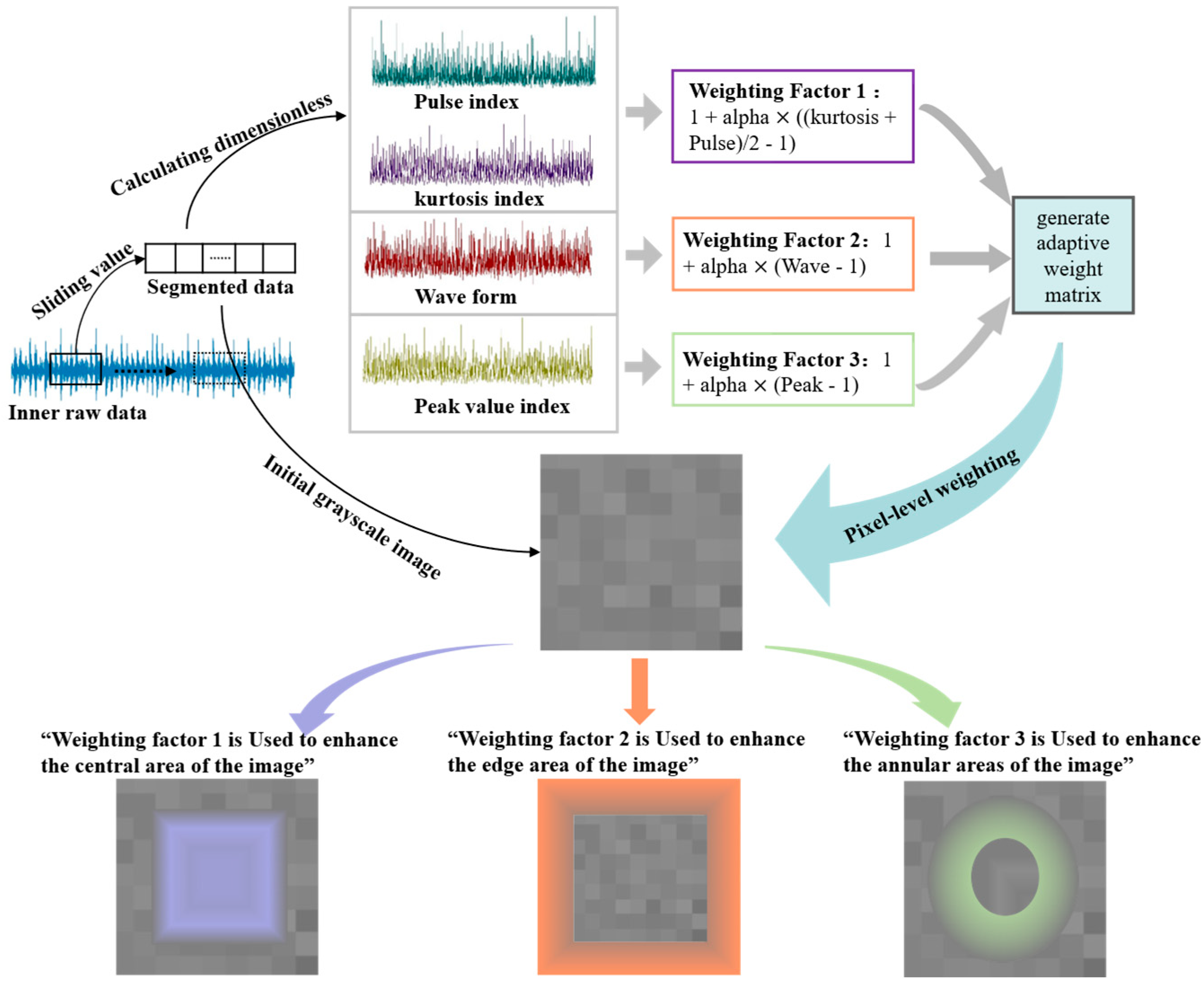
The distribution of fault characteristic frequencies is determined by the physical structure of the bearing, as shown in Equations (2)–(4) [26]. The characteristic frequencies vary depending on the specific faulty component. According to Equation (2), when an inner race defect occurs, term $(1+{\displaystyle \frac{d\cos \alpha }{D}})$ becomes dominant, resulting in a higher fault frequency relative to term $f_r$. As a result, the corresponding high-impact signals are more sensitive to kurtosis and impulse factor indicators. Therefore, the grayscale image weighting is configured to emphasize the central region; According to Equation (3), when an outer race defect occurs, term $(1-{\displaystyle \frac{d\cos \alpha }{D}})$ is reduced, resulting in a relatively moderate fault frequency. In this case, waveform indicators are more sensitive to steady-state periodic signals, and the grayscale weighting is applied to an annular region along the image edges. According to Equation (4), when a rolling element defect occurs, it is affected by term $\mathrm{D}/\mathrm{d}$, leading to a moderately high fault frequency. As a result, peak value indicators become more sensitive to intermittent impacts, and the grayscale weighting is assigned to a central annular region, as illustrated in Figure 1.

$$\mathrm{Inner} \mathrm{race} \mathrm{fault} \mathrm{frequency}: f_{BPFI}={\displaystyle \frac{N}{2}}(1+{\displaystyle \frac{d\cos \alpha }{D}})f_r$$

(2)

$$\mathrm{Outer} \mathrm{race} \mathrm{fault} \mathrm{frequency}: f_{BPFO}={\displaystyle \frac{N}{2}}(1-{\displaystyle \frac{d\cos \alpha }{D}})f_r$$

(3)

$$\mathrm{Rolling} \mathrm{element} \mathrm{failure} \mathrm{frequency}: f_{BPFr}={\displaystyle \frac{D}{2d}}(1-{({\displaystyle \frac{d\cos \alpha }{D}})}^2)f_r$$

(4)

3.2. Dimensionless Weighted Grayscale Image

As shown in Figure 2, to obtain the dimensionless grayscale weighted image. $G^{*}(i,j)$, the bearing vibration signal. $X_1$ is first resampled using a sliding window and converted into a grayscale image with dimensions M × M. The center coordinate of the grayscale image is calculated as C = M/2. Meanwhile, the weight matrix $W(i,j)$ is initialized to 1, with $\forall i,j\in [0,M-1]$. Meanwhile, the bearing vibration data $X_1$ is segmented using the same sliding window, and the dimensionless indicators are calculated for each segment based on its fault type.

According to Equation (5), center-region weighting is applied to the grayscale image, where a is a parameter used to define the size of the central region, $I_f$ denotes the impulse factor, ${\mathrm{K}}_{\mathrm{v}}$ represents the kurtosis factor [25], and $\alpha$ is a tuning coefficient that adjusts the weighting intensity within the specified region. The definition of $\alpha$ remains consistent in the subsequent equations.

$$W(i,j)=W(i,j)\cdot [1+\alpha ({\displaystyle \frac{K_v+I_f}{2}}-1)], |i-C|\le a, |j-C|\le a$$

(5)

According to Equation (6), annular edge-region weighting is applied to the grayscale image, where b is a parameter that defines the size of the edge region, and $S_f$ denotes the waveform factor [25].

$$W(i,j)=W(i,j)\cdot [1+\alpha (S_f-1)], i\le b\vee j\le b\vee i\ge M-b\vee j\ge M-b$$

(6)

Equation (7) applies annular center-region weighting, where c is a parameter that defines the size of the central annular region, and $C_f$ represents the peak value factor [25].

$$W(i,j)=W(i,j)\cdot [1+\alpha (C_f-1)], \mathrm{D}=\sqrt{{(\mathrm{i}-\mathrm{C})}^2+{(\mathrm{j}-\mathrm{C})}^2}, c\le D\le C-c$$

(7)

After completing the dimensionless grayscale weighting for different fault types, max normalization is performed according to Equation (8) to obtain the grayscale weighting factors. The final dimensionless weighted grayscale image $G^{*}(i,j)$ is then generated.

$$\widehat{W}(i,j)={\displaystyle \frac{W(i,j)}{\max (W(i,j))}}$$

(8)

3.3. Cheap Channel Obfuscation Module

Standard convolution operations are computationally expensive. To reduce computational load and free up processing resources, Han [27] proposed a method in which a small portion of standard convolutions is used to generate primary features, while redundant features are simulated using low-cost operations to mimic additional channels.

In this paper, a strategy is proposed that integrates redundant features generated through cheap operations with a channel confusion mechanism [24] to enhance channel interaction and improve feature representation. This approach effectively increases the utilization efficiency of the dimensionless weighted grayscale maps while maintaining low computational cost.

As shown in Figure 3, the dimensionless grayscale-weighted map G is decoupled and separated into signal and noise components via convolution: [${\mathrm{G}}_{\mathrm{signal}}\in {ℝ}^{H\times W\times C_{\mathrm{in}}}$, ${\mathrm{G}}_{\mathrm{noise}}\in {ℝ}^{H\times W\times C_{\mathrm{in}}}$] = CONV1$\times$1($\mathrm{G}\in {ℝ}^{H\times W\times C_{\mathrm{in}}}$), where $ℝ$ denotes the real space, H and W represent the data dimensions, and C indicates the number of input channels. ${\mathrm{G}}_{\mathrm{signal}}$ undergoes a cheap linear operation to extract redundant features, yielding Y₁. $G_{noise}$ is subjected to noise suppression: Y₂ = b $\times$ $G_{noise}$.

Finally, Y₁ and Y₂ are channel-shuffled according to the group number to produce Y. This network design enhances feature representation in the signal pathway while suppressing noise in the noise pathway, thereby improving robustness. Without requiring additional parameters, it boosts model expressiveness and meets lightweight requirements.

3.4. Model Structure

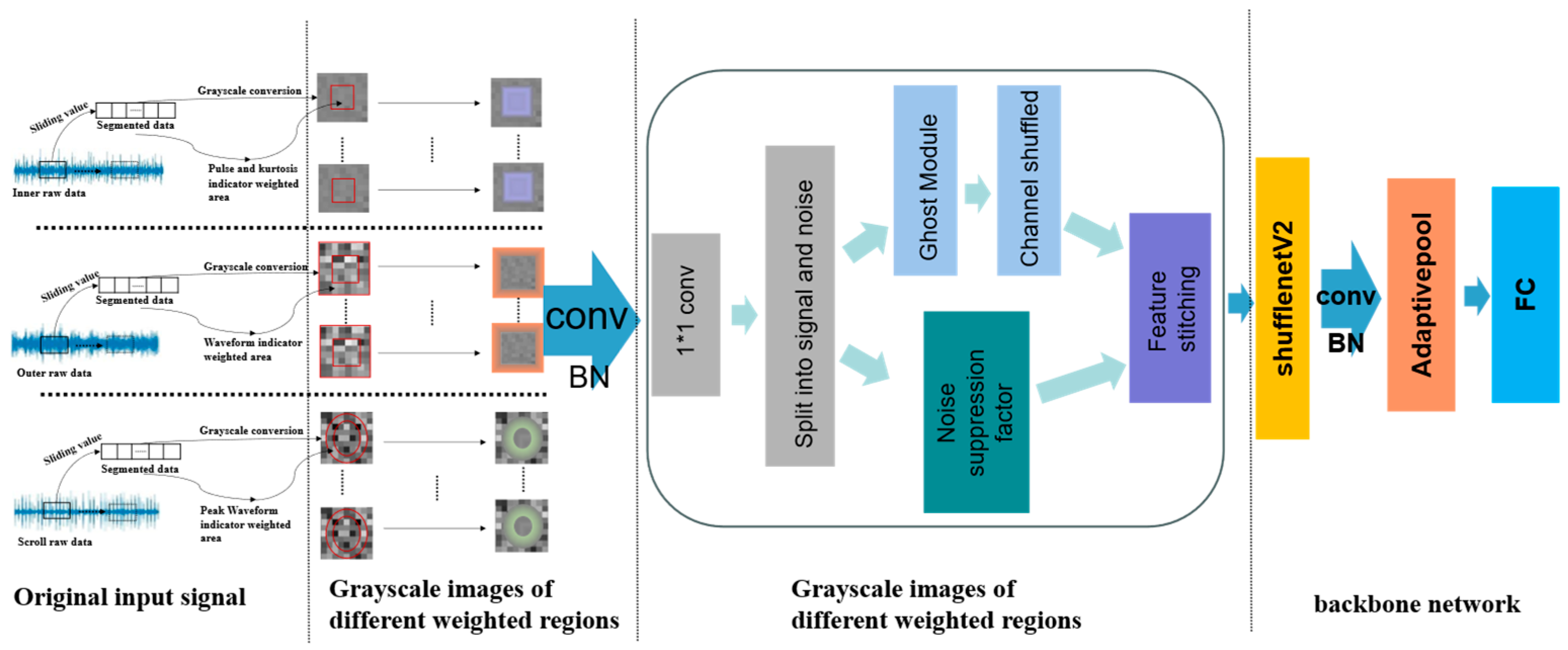
To achieve efficient fault identification and model lightweighting for rolling bearings, this paper proposes a lightweight fault diagnosis model named ADGCC-Net. The model integrates three key components: a dimensionless grayscale mapping-based feature representation method (Section 3.1 and Section 3.2), a Cheap channel obfuscation module (Section 3.3), and the backbone network ShuffleNetV2. Through the effective integration of these lightweight modules, the overall parameter size of the model is controlled at 0.0822 MB. The detailed architecture is illustrated in Figure 4.

The complete diagnostic procedure is as follows: First, the collected bearing vibration signals are converted into grayscale images and resampled using a sliding window. Simultaneously, the same sliding window is used to sample the vibration signals and compute dimensionless indicators. These indicators are then used to perform key region weighting on the corresponding grayscale images, resulting in dimensionless weighted grayscale maps for different fault locations of the bearing. A Cheap channel obfuscation module is introduced before the ShuffleNetV2 network to ensure low parameter complexity while enabling redundant feature generation and enhancing inter-channel feature interaction. The network outputs are then passed through an adaptive pooling layer and a fully connected layer for dimensionality reduction, producing the number of fault categories for the dataset. Finally, a linear classifier is used for fault recognition, enabling the identification of the current fault type.

In order to better understand the dimensionless weighted grayscale image construction process and principle, it is described in detail in Section 3.1 and Section 3.2, and the cheap channel confusion module is described in detail in Section 3.3.

4. Experiment

4.1. Datasets

The experimental data used in this study are sourced from the bearing dataset developed by the Bearing Data Center of Case Western Reserve University (CWRU) [28]. The dataset includes bearing vibration signals under various fault modes and load conditions. For each fault diameter, three fault types are provided: inner race fault, rolling element fault, and outer race fault. This study utilizes data collected from the drive-end bearing. The sampling frequency is 12 kHz, and each condition contains 119,808 data points. The fault diameters (in inches) are 0.007, 0.014, and 0.021, with a total of ten bearing conditions. Additionally, datasets under four different load conditions—0 HP, 1 HP, 2 HP, and 3 HP—are used for comparative experiments.

The experimental data used in this study are sourced from the Southeast University (SEU) dataset [29]. The SEU bearing dataset was collected using a transmission system dynamics simulator and includes vibration data under two different operating conditions: 20 Hz-0 V and 30 Hz-2 V. This study utilizes vibration data in the X-direction. The dataset contains five fault categories, including rolling element, inner race, and outer race faults, with 341,333 sample points for each condition. Datasets under two different load conditions—0 HP and 2 HP—were used for comparative experiments.

4.2. Experimental Environment

This experiment uses an environment built by a cloud server. Specifications: GPU: RTX 2080Ti; Memory: 40 GB; Image environment: Python 3.12 (ubuntu22.04), Cuda12.1, PyTorch 2.3.2.

The architectural details of the proposed ADGCC-Net are systematically presented in

Table 1. ADGCC-Net structure parameters.

Structure	Output	Kernel Size	Step	Padding
Input	32 × 32
Conv2d	32 $\times$ 32 $\times$ 32	3 $\times$ 3	2	1
BN	32 $\times$ 32 $\times$ 32
Stage1	32 $\times$ 16 $\times$ 16 32 $\times$ 16 $\times$ 16		2 2	0 0
Conv2d	1024 $\times$ 16 $\times$ 16	1 $\times$ 1	1	0
BN	1024 $\times$ 16 $\times$ 16
AdaptiveAvgPool2d	1024 $\times$ 1 $\times$ 1
FC	10

. The network processes bearing vibration signals converted into 32 × 32 grayscale images through our novel physics-informed transformation method described in Section 3.1. The architecture employs a strategic combination of spatial reduction and channel expansion operations, with particular emphasis on computational efficiency through grouped pointwise convolutions.

Input Representation: The network accepts preprocessed 2D representations (32 × 32 pixels) where vibration characteristics are encoded through dimensionless indicator weighting. Initial Feature Extraction: The first convolutional layer (Conv2d) utilizes 32 filters with a 3 × 3 kernel (stride = 2, padding = 1) to extract preliminary spatial features while reducing spatial dimensions by half through strided convolution. Batch normalization follows immediately to stabilize gradient propagation and accelerate convergence. Multi-Scale Feature Learning: Stage1 further processes features through a series of operations that maintain channel depth (32) while reducing spatial resolution to 16 × 16, likely incorporating pooling or additional strided convolutions. Grouped Pointwise Convolution Layers: Conv1 (implied in initial layers): Although not explicitly labeled in this table, our implementation incorporates grouped pointwise convolution principles in early stages to establish efficient feature foundations. Conv5 (channel expansion layer): A critically designed grouped 1 × 1 convolution (groups = 32) dramatically expands channel dimensionality from 32 to 1024 while preserving spatial resolution (16 × 16). This operation achieves a 98.5% parameter reduction compared to standard convolutional approaches, requiring only 1024 parameters instead of the theoretical 32 × 1024 = 32,768 parameters of a conventional implementation. Global Feature Aggregation: Adaptive average pooling collapses spatial dimensions to 1 × 1, transforming the 1024-channel feature maps into a compact 1024-dimensional representation vector. Classification Head: A fully connected layer maps the high-level features to 10 output neurons, corresponding to the fault categories in our experimental setup (9 fault types plus normal condition).

4.3. Results on CWRU

The rolling bearing dataset was split into non-overlapping training and testing sets at a ratio of 0.3:0.2. A sliding window was applied to resample the data, resulting in 1008 dimensionless weighted grayscale images for the training set and 672 images for the testing set. For the experiments, the input batch size was set to 32, the learning rate was 0.0018, the activation function was ReLU, and the loss function was Cross Entropy Loss. The Adam optimizer was employed to update the network parameters via backpropagation over 60 training epochs.

4.3.1. Model Testing and Analysis

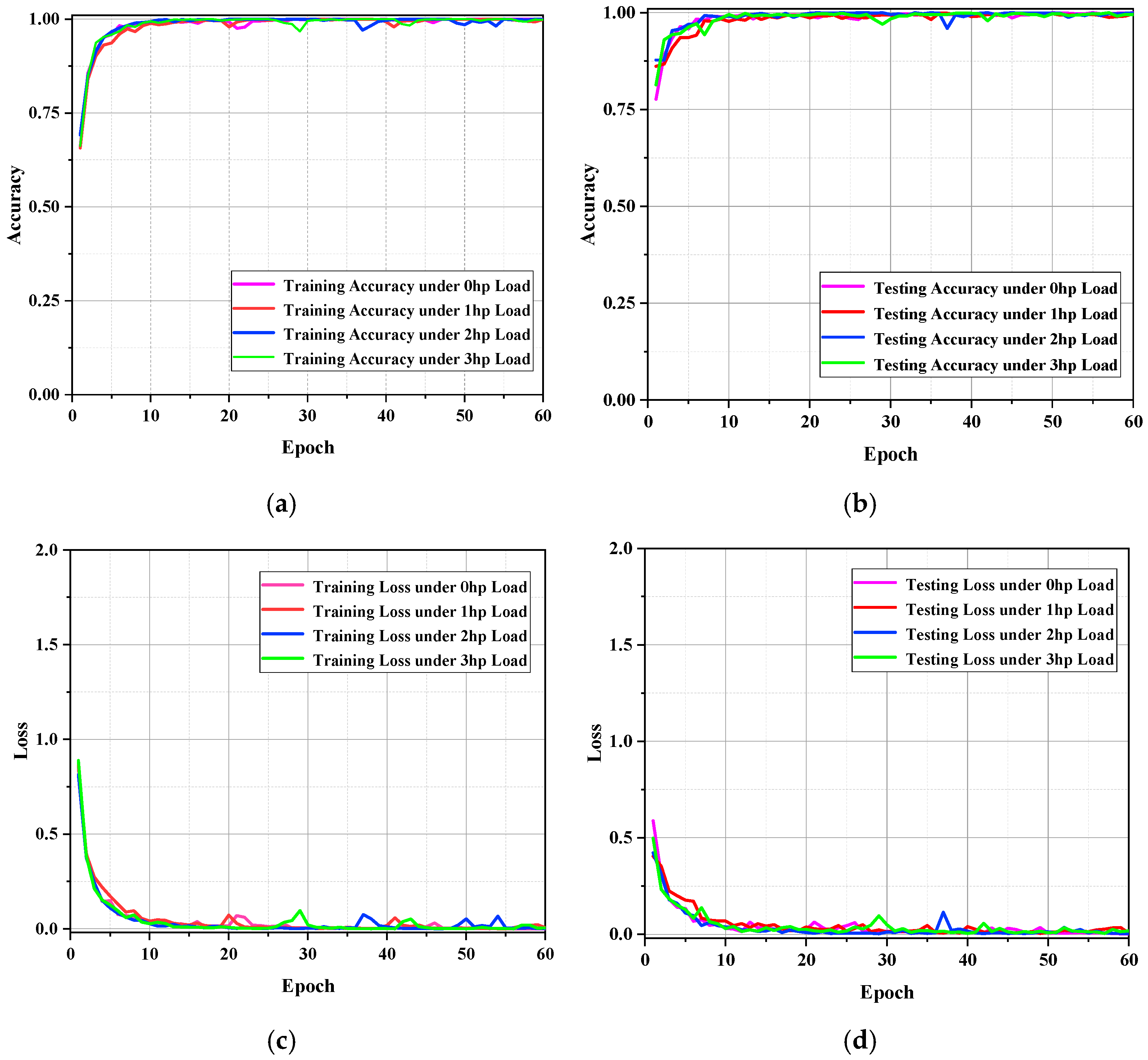
When the adjustment parameter $\alpha$ was set to 1—representing a fully weighted strategy—the experimental results are shown in Figure 5. This figure illustrates the trends in loss and accuracy during training under various load conditions using the CWRU bearing dataset.

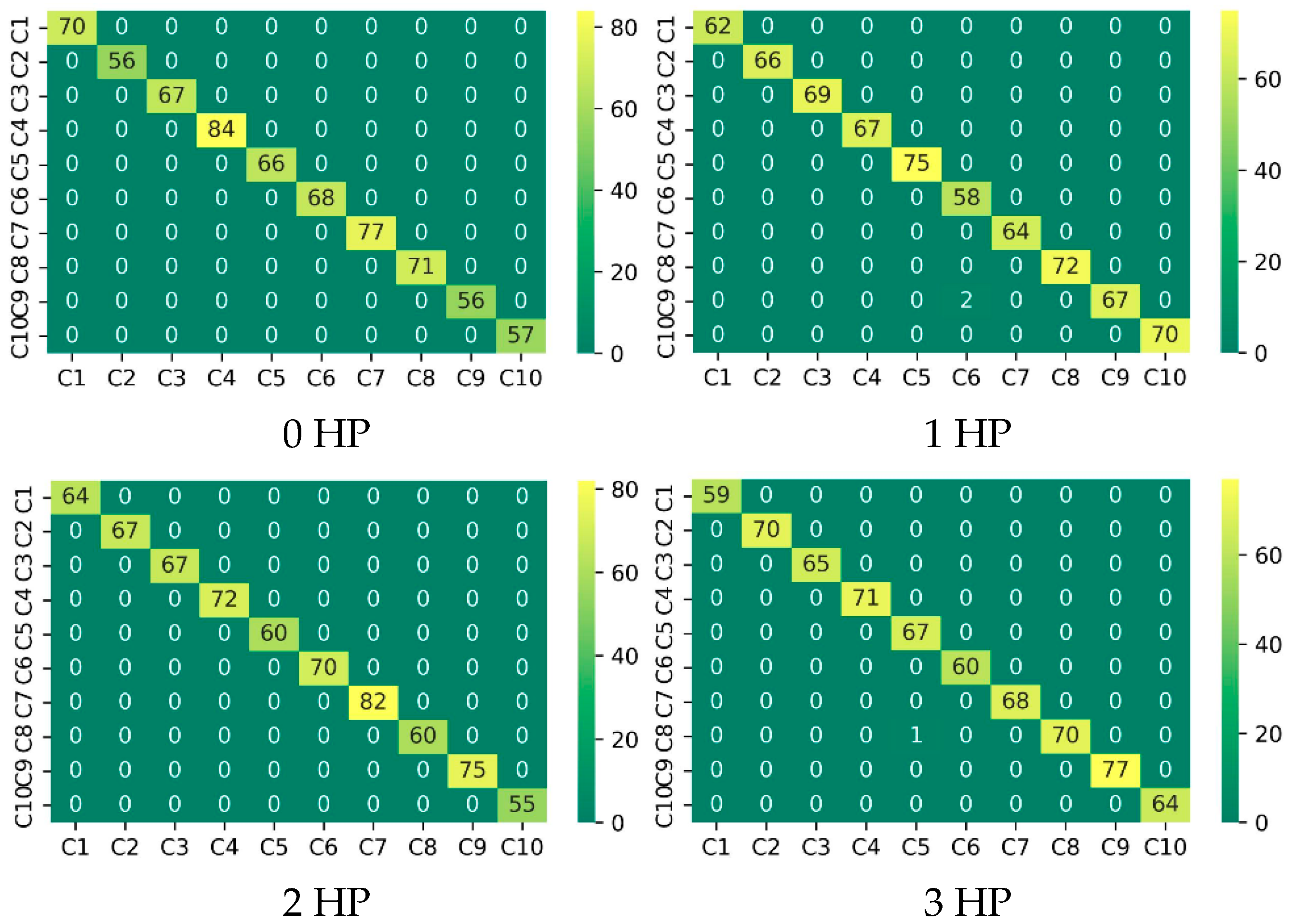
Confusion matrices [30] were plotted based on the predicted and actual labels of the test data under load conditions of 0 HP, 1 HP, 2 HP, and 3 HP, as shown in Figure 6. In the figure, the horizontal axis represents the predicted classes, while the vertical axis represents the actual classes.

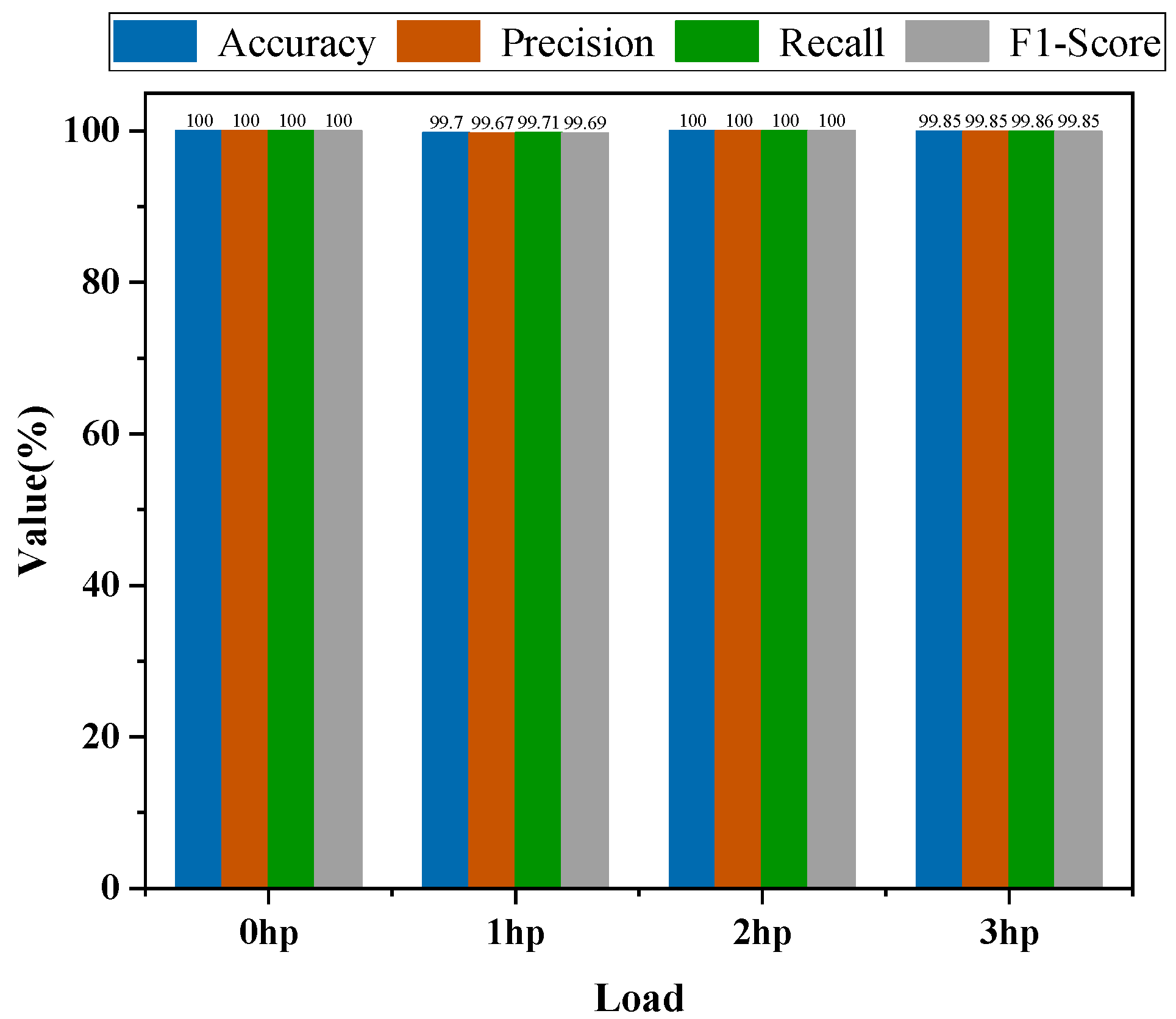
To quantitatively evaluate the model’s overall performance under different load conditions, we calculated four key evaluation metrics—Accuracy, Precision, Recall, and F1-Score [31]—based on the confusion matrix shown in Figure 6. The results for the four load conditions are summarized as bar charts in Figure 7.

Based on the confusion matrix, the model demonstrates excellent overall recognition performance in the ten-class classification task under different load conditions. The key classification performance metrics derived from the confusion matrix remain at consistently high levels, indicating that the model possesses strong feature discrimination and generalization capabilities, effectively distinguishing between different fault categories. Furthermore, the training and testing accuracy curves are highly consistent, both exceeding 99% at an early stage and remaining stable thereafter, highlighting the model’s strong generalization ability and robustness. In summary, the proposed ADGCC-Net model exhibits outstanding fault diagnosis performance on the CWRU dataset across various load conditions.

4.3.2. Accuracy Comparison of Different Models Based on CWRU Data

To validate the superiority of the proposed method, this study selected several representative diagnostic approaches from recent research on the CWRU bearing dataset for comparative experiments, as shown in

Table 2. Comparative experiment.

Model\Load	0 HP	1 HP	2 HP	3 HP	Param/105
ResNet [32]	0.9973	0.9835	0.9880	0.9800	21.3
MobileNet [33]	0.9480	0.9588	0.9579	0.9024	0.54
EfficientNet [34]	0.9721	0.9818	0.9522	0.9339	5.31
ShuffleNet [35]	0.9723	0.9725	0.9646	0.9556	5.39
Ours	1.0000	0.9970	1.0000	0.9985	0.21

. Under the same experimental conditions, when the load levels were 0 HP, 1 HP, 2 HP, and 3 HP, the corresponding modulation factors were set to 0.4, 0.6, 0.6, and 0.2, respectively. At this point, our model achieves the highest diagnostic accuracy under different operating conditions, with the accuracy reaching 1.0 particularly under the 2 HP and 3 HP load conditions. These results demonstrate that the proposed modulation mechanism can effectively adapt to variations in load conditions and significantly enhance the model’s adaptability to diverse operating scenarios.

4.4. Result on SEU

The rolling bearing dataset was divided into non-overlapping training and testing sets in a 0.3:0.2 ratio. Using a sliding window for data resampling, 1632 dimensionless weighted grayscale images were generated for the training set and 1088 images for the testing set. For the experiments, the input batch size was set to 32, the learning rate to 0.002, the activation function used was ReLU, and the loss function was Cross Entropy Loss. The network parameters were optimized using the Adam algorithm over 80 training epochs.

4.4.1. Model Testing

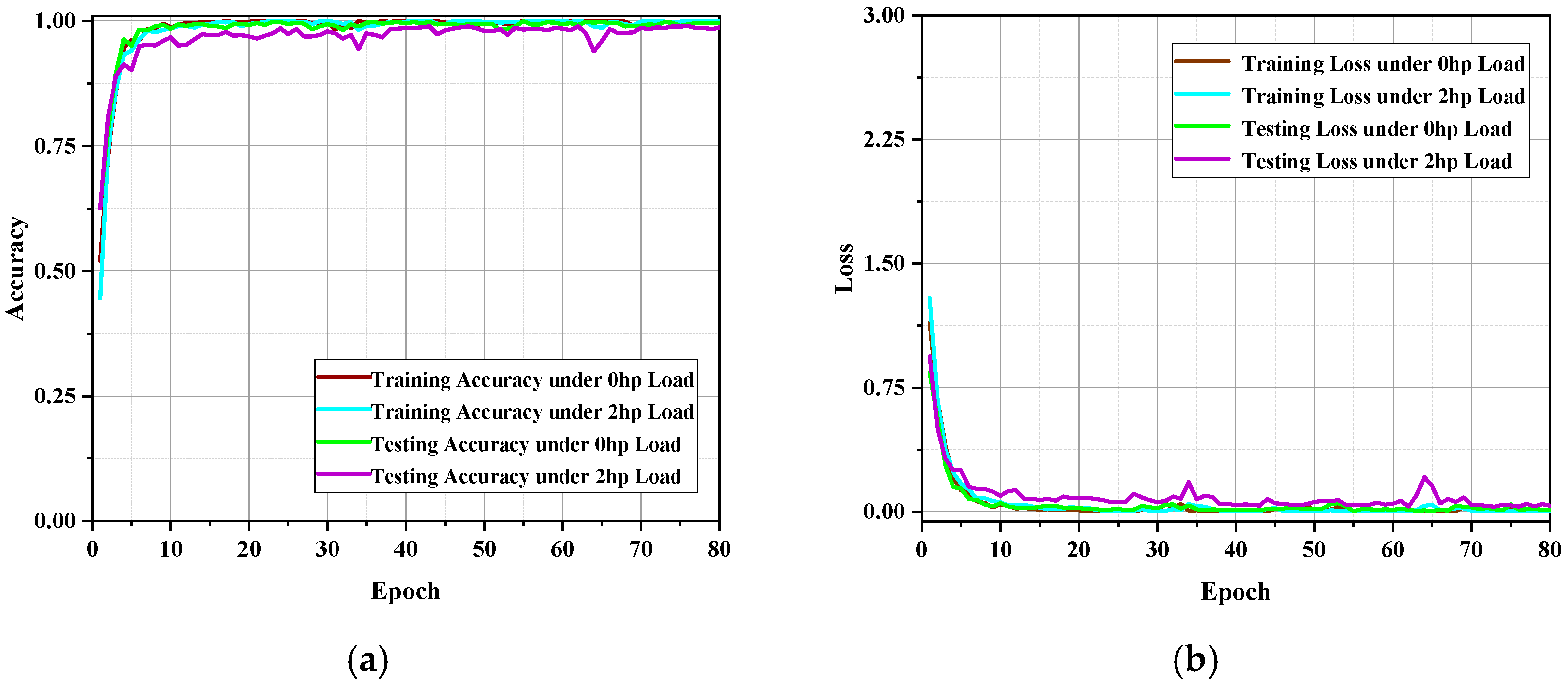
When the modulation factor $\alpha$ was set to 0.8—i.e., applying the 0.8-weighting strategy—the experimental results are shown in Figure 8, which illustrates the trends of the model’s loss and accuracy across training epochs under different load conditions using the SEU bearing dataset.

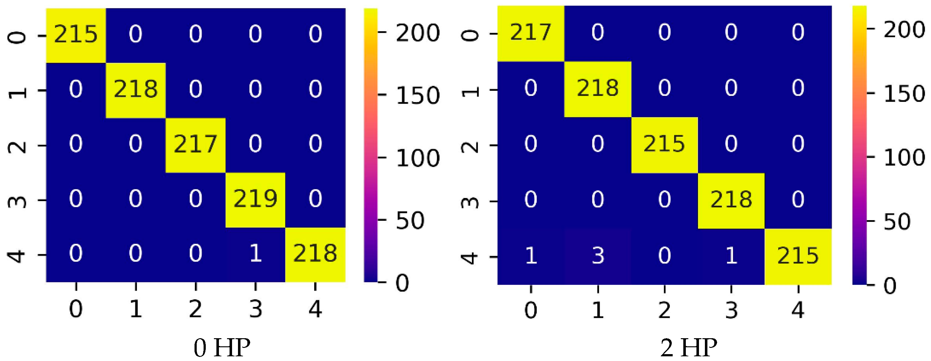
Based on the test results under 0 HP and 2 HP loading conditions, the confusion matrices were plotted using the predicted and actual labels, as shown in Figure 9. The horizontal axis represents the predicted classes, while the vertical axis indicates the actual classes. As observed, the ADGCC-Net model demonstrates excellent fault diagnosis performance on the SEU bearing dataset.

4.4.2. Accuracy Comparison of Different Models Based on SEU Data

To validate the superiority of the proposed approach, representative diagnostic methods for the SEU bearing dataset from recent years were selected for comparative experiments, as summarized in

Table 3. Comparative experiment.

Model\Load	0 HP	Param (MB)
MCDS-CNN [36]	0.9980	1.58
2D-CNN [36]	0.7680	62.32
MobileNet [36]	0.9280	21.01
Ours	0.9991	0.0822

. Under the same experimental conditions, when the load was 0 HP and the modulation factor was set to $\alpha$ = 0.8, the proposed model achieved a diagnostic accuracy of 99.91%. These results indicate that the proposed modulation mechanism effectively adapts to varying load conditions and significantly enhances the model’s adaptability to different working environments.

4.5. Modulatory Factor Experiment

To evaluate the robustness and generalization capability of the model, moderate-intensity noise was introduced solely into the CWRU, with a signal-to-noise ratio (SNR) of 15 dB. On this basis, a linear weighting model controlled by the modulation factor $\alpha$ was constructed and incorporated into the feature fusion process of dimensionless indicators, aiming to enhance the model’s responsiveness to key regional features. The linear weighting model is defined as $W(i,j)=W(i,j)\cdot [1+\alpha (\varphi -1)]$, where $\varphi$ represents the indicator value. As shown in

Table 4. At SNR = 15 dB, the accuracy corresponding to different α.

Load\α	0	0.2	0.4	0.6	0.8	1
0 HP	0.9805	0.9896	0.9948	0.9909	0.9857	0.9922
1 HP	0.9740	0.9792	0.9844	0.9857	0.9857	0.9792
2 HP	0.9909	0.9948	0.9987	1.0000	1.0000	0.9935
3 HP	0.9948	0.9857	0.9974	0.9974	0.9961	0.9948

, the model was validated under various operating conditions to analyze the impact of introducing the modulation factor $\alpha$ on fault recognition accuracy, thereby assessing the model’s generalization performance across different scenarios. A comparison between full weighting ($\alpha$ = 1) and no weighting ($\alpha$ = 0) demonstrates that the model achieved a maximum accuracy of 1.

The comparative analysis of the above data indicates that the proposed method can effectively adapt to fault diagnosis tasks under various operating conditions through appropriate adjustment of the modulation factor $\alpha$, demonstrating strong generalization performance.

The impact of introducing the modulation factor $\alpha$ on fault identification accuracy was systematically analyzed to evaluate the generalization capability and adaptability of the proposed model. As shown in

Table 5. The accuracy corresponding to different α.

Load\α	0	0.2	0.4	0.6	0.8	1
0 HP	0.9688	0.9871	0.9908	0.9945	0.9982	0.9931
2 HP	0.9642	0.9853	0.9862	0.9908	0.9954	0.9908

, diagnostic accuracy was experimentally validated on the SEU bearing dataset under various working conditions. When comparing the fully weighted strategy ($\alpha$ = 1) with the non-weighted one ($\alpha$ = 0), the model’s accuracy increased by approximately 3%.

4.6. Ablation Study

To verify the effectiveness of the proposed dimensionless grayscale-weighted image construction and the cheap channel obfuscation module on the CWRU bearing dataset, experiments were conducted under a signal-to-noise ratio (SNR) of 15 dB and a load condition of 0, with the modulation factor $\alpha$ set to 1. The proposed grayscale image construction method was compared with a baseline approach in which the original data was directly converted into grayscale images. As shown in

Table 6. Comparison of Ablation Experiments Based on CWRU Data.

Ablation Network Comparison	Recognition Accuracy
Original signal + ShuffleNetV2	0.9688
Grayscale image + ShuffleNetV2	0.9766
Dimensionless weighted grayscale image + ShuffleNetV2	0.9870
Original signal + Cheap channel obfuscation module + ShuffleNetV2	0.9792
Grayscale image + Cheap channel obfuscation module + ShuffleNetV2	0.9805
This model	0.9922

, the proposed method achieved the highest diagnostic accuracy. Moreover, the ablation study demonstrates that the proposed dimensionless grayscale-weighted images significantly enhance time-frequency representation robustness by normalizing time-frequency energy distributions and focusing weights on key frequency bands, maintaining an identification accuracy above 98.5% even in noisy environments.

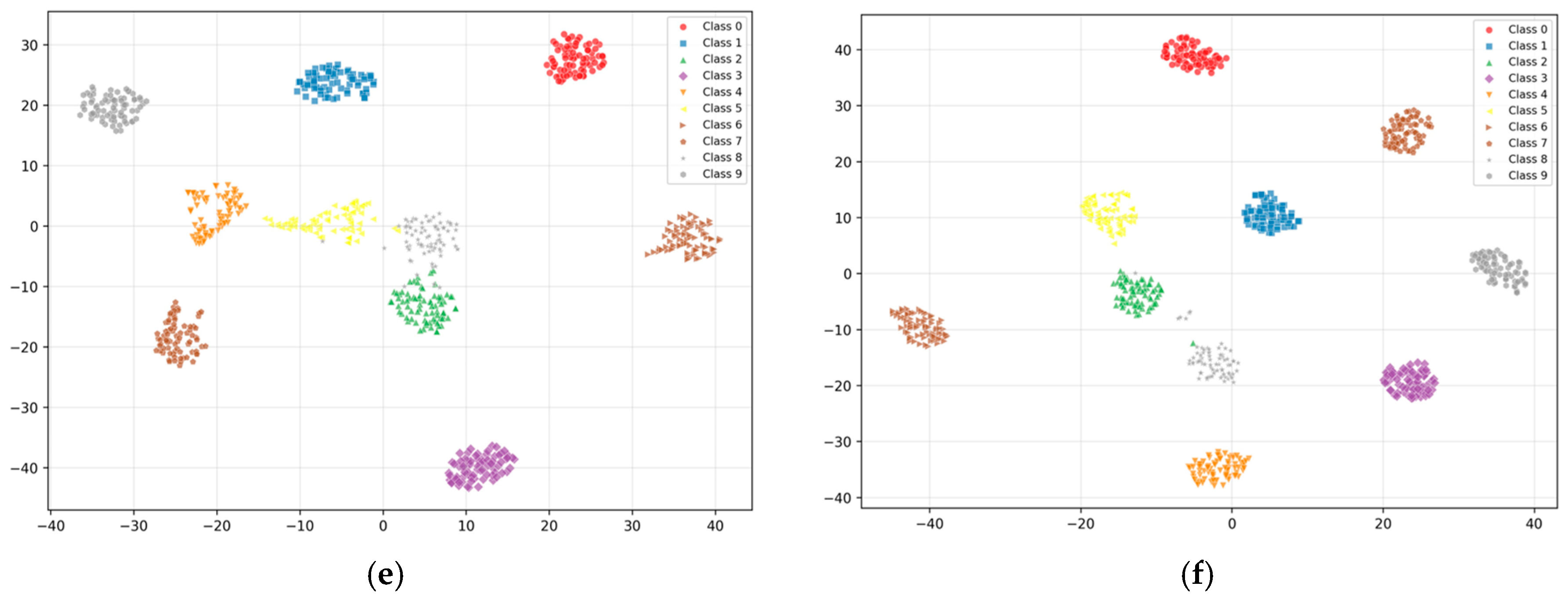
Based on the above experiments, by extracting features from the AdaptiveAvgPool2d layer of the model and using t-SNE technology for feature visualization, as shown in Figure 10, the features learned by the model equipped with the Cheap Channel Obfuscation Module exhibit tighter intra-class clustering and clearer inter-class separability compared to the baseline model, indicating a higher discriminative capability of the extracted representations. This validates that the proposed module effectively enhances feature diversity.

To further demonstrate the effectiveness of the proposed dimensionless grayscale weighting map and the Cheap channel obfuscation module on the SEU bearing dataset, an experimental comparison was conducted under the 0 HP load condition with the modulation factor set to $\alpha$ = 0.8. The proposed grayscale weighting construction method was compared to the direct grayscale transformation of raw data. As shown in

Table 7. Comparison of Ablation Experiments Based on SEU Data.

Ablation Network Comparison	Recognition Accuracy
Original signal + ShuffleNetV2	0.9651
Grayscale image + ShuffleNetV2	0.9606
Dimensionless weighted grayscale image + ShuffleNetV2	0.9899
Original signal + Cheap channel obfuscation module + ShuffleNetV2	0.9761
Grayscale image + Cheap channel obfuscation module + ShuffleNetV2	0.9688
This model	0.9982

, the proposed method achieved the highest diagnostic accuracy. Additionally, ablation experiments revealed that the proposed dimensionless grayscale weighting approach significantly enhanced the robustness of time-frequency representations by normalizing the energy distribution and emphasizing key frequency bands, maintaining a recognition accuracy above 98.9% under noisy conditions.

Based on the above experiments, the features of the AdaptiveAvg-Pool2d layer of the model were visualized using t-SNE technology (as shown in Figure 11). Compared with the baseline model, the features learned by the model equipped with the inexpensive channel confusion module showed tighter intra-class clustering and clearer inter-class separability, indicating that the extracted feature representation has higher discriminative power. This also demonstrates the model’s strong generalization ability.

4.7. Discuss

While deep learning has advanced bearing fault diagnosis, significant gaps remain in constructing physically meaningful inputs and learning robust, lightweight representations. Firstly, in conventional signal-to-image transformation, the generated grayscale representations often lack physical correspondence with the actual vibration source locations, leading to ambiguous feature distributions. Moreover, these methods frequently overlook crucial statistical characteristics of vibration signals, such as kurtosis and impulsiveness, which are vital indicators of mechanical health. Secondly, even with improved inputs, feature representations often suffer from noise interference and redundant channel coupling, which degrade discriminability and inflate model complexity. Compounding this, lightweight networks designed for efficiency tend to lose critical fault information during feature compression.

Our work directly addresses these gaps. To bridge the first, we introduce a physics-guided image construction strategy that embeds physical prior knowledge by using dimensionless indicators to adaptively weight image regions, ensuring the transformation maintains physical consistency and diagnostic relevance. To address the second, we propose a Cheap Channel Obfuscation module within a unified framework, achieving simultaneous noise suppression, channel decorrelation, and lightweight feature enhancement without significant information loss.

It is also important to contextualize the limitations and future directions of our approach, which further define the current research frontier. The model’s performance is influenced by empirically set preprocessing parameters (e.g., sliding window length, overlap ratio), whose optimal values are likely dataset-specific. Furthermore, while our model shows high efficacy on single, stationary faults, its performance on compound faults or evolving progressive faults—more complex, real-world scenarios—requires further investigation and could necessitate multi-label or temporal modeling extensions. Architecturally, the aggressive initial spatial downsampling, though beneficial for efficiency, poses a potential trade-off by potentially attenuating subtle, high-frequency fault signatures—a challenge that future work could address with parallel branch structures designed to preserve fine details. These points collectively underscore both the advancements made by our present study and the precise trajectory for future research.

5. Conclusions

This study has presented two key contributions for advancing bearing fault diagnosis. Through extensive experimental validation, the following conclusions are drawn:

The proposed construction method of the dimensionless weighted grayscale map integrates grayscale representations of bearing vibration signals with dimensionless feature indicators extracted from different signal positions. By introducing prior physical knowledge to modulate the spatial distribution of grayscale features, the model’s attention to critical fault regions is significantly enhanced, thereby improving overall diagnostic accuracy and discriminative capability. The proposed scheme demonstrates strong performance, consistently achieving diagnostic accuracy above 96.88% on both the CWRU and SEU datasets after converting the raw signals into image data.

The proposed cheap channel obfuscation module combines the low-cost feature generation mechanism of the Ghost module with the channel reorganization strategy of ShuffleNetV2. This design effectively strengthens inter-channel information interaction and feature expression efficiency while maintaining low computational complexity and achieving a highly efficient and lightweight network architecture. Compared to the baseline, the incorporation of the proposed module yielded a 1% gain in recognition accuracy. The features from the pooling layer exhibit improved inter-class separation, confirming its effectiveness in learning more discriminative representations.

The proposed method demonstrates promising performance in bearing fault diagnosis; however, its effectiveness is highly dependent on choices made during the data preprocessing stage. Parameters such as sliding window length, overlap ratio, and weighting factors in the indicator matrix are set empirically, and their optimal values are likely influenced by rotational speed, bearing type, and fault severity. Future work should focus on developing adaptive parameter determination mechanisms to improve generalization.

References

1. Mongia, C.; Goyal, D.; Sehgal, S. Vibration response-based condition monitoring and fault diagnosis of rotary machinery. Mater. Today Proc. 2022, 50, 679–683. [Google Scholar] [CrossRef]
2. Murgia, A.; Verbeke, R.; Tsiporkova, E.; Terzi, L.; Astolfi, D. Discussion on the suitability of SCADA-based condition monitoring for wind turbine fault diagnosis through temperature data analysis. Energies 2023, 16, 620. [Google Scholar] [CrossRef]
3. Wang, N. Bearing Fault Diagnosis Based on SMA-VMD and CNN-LSTM. Int. J. Comput. Sci. Inf. Technol. 2024, 2, 100–109. [Google Scholar] [CrossRef]
4. Zhang, Q.; Deng, L. An intelligent fault diagnosis method of rolling bearings based on short-time Fourier transform and convolutional neural network. J. Fail. Anal. Prev. 2023, 23, 795–811. [Google Scholar] [CrossRef]
5. Li, H.; Liu, T.; Wu, X.; Chen, Q. An optimized VMD method and its applications in bearing fault diagnosis. Measurement 2020, 166, 108185. [Google Scholar] [CrossRef]
6. Han, D.; Chen, H.; Chen, X.; Wang, J.; Wei, L. Fault diagnosis of rolling bearings based on short-time Fourier transform and DRSN. China Meas. Test 2024, 50, 136–141. [Google Scholar]
7. Zhang, G.; Li, Y.; Zhao, Y. A novel fault diagnosis method for wind turbine based on adaptive multivariate time-series convolutional network using SCADA data. Adv. Eng. Inform. 2023, 57, 102031. [Google Scholar] [CrossRef]
8. Wang, Z.; Wu, Z.; Li, X.; Shao, H.; Han, T.; Xie, M. Attention-aware temporal–spatial graph neural network with multi-sensor information fusion for fault diagnosis. Knowl.-Based Syst. 2023, 278, 110891. [Google Scholar] [CrossRef]
9. Cui, J.; Xie, P.; Wang, X.; Wang, J.; He, Q.; Jiang, G. M2FN: An end-to-end multi-task and multi-sensor fusion network for intelligent fault diagnosis. Measurement 2022, 204, 112085. [Google Scholar] [CrossRef]
10. Qin, S.; Tao, J.; Zhao, Z. Fault diagnosis of wind turbine pitch system based on LSTM with multi-channel attention mechanism. Energy Rep. 2023, 10, 4087–4096. [Google Scholar] [CrossRef]
11. Liang, J.; Zhang, K.; Al-Durra, A.; Zhou, D. A multi-information fusion algorithm to fault diagnosis of power converter in wind power generation systems. IEEE Trans. Ind. Inform. 2023, 20, 1167–1179. [Google Scholar] [CrossRef]
12. Huo, D.; Kang, Y.; Wang, B.; Feng, G.; Zhang, J.; Zhang, H. Gear fault diagnosis method based on multi-sensor information fusion and VGG. Entropy 2022, 24, 1618. [Google Scholar] [CrossRef]
13. Li, N.; Wang, H. Variable Filtered-Waveform Variational Mode Decomposition and Its Application in Rolling Bearing Fault Feature Extraction. Entropy 2025, 27, 277. [Google Scholar] [CrossRef]
14. Li, T.; Shi, H.; Bai, X.; Li, N.; Zhang, K. Rolling bearing performance assessment with degradation twin modeling considering interdependent fault evolution. Mech. Syst. Signal Process. 2025, 224, 112194. [Google Scholar] [CrossRef]
15. Liang, P.; Wang, B.; Jiang, G.; Li, N.; Zhang, L. Unsupervised fault diagnosis of wind turbine bearing via a deep residual deformable convolution network based on subdomain adaptation under time-varying speeds. Eng. Appl. Artif. Intell. 2023, 118, 105656. [Google Scholar] [CrossRef]
16. Wang, M.-H.; Lu, S.-D.; Hsieh, C.-C.; Hung, C.-C. Fault detection of wind turbine blades using multi-channel CNN. Sustainability 2022, 14, 1781. [Google Scholar] [CrossRef]
17. Xie, K.; Cheng, C.; Cheng, Y.; Wang, Y.; Chen, L. LFDNet: A lightweight fault diagnosis network for wind turbine gearboxes. Meas. Sci. Technol. 2025, 36, 036139. [Google Scholar] [CrossRef]
18. Cheng, X.; Dou, S.; Du, Y.; Wang, Z. Gearbox fault diagnosis method based on lightweight channel attention mechanism and transfer learning. Sci. Rep. 2024, 14, 743. [Google Scholar] [CrossRef]
19. Dong, Y.; Wen, C.; Wang, Z. A motor bearing fault diagnosis method based on multi-source data and one-dimensional lightweight convolution neural network. Proc. Inst. Mech. Eng. Part I J. Syst. Control. Eng. 2023, 237, 272–283. [Google Scholar] [CrossRef]
20. Cai, C.; Xu, T.; Ren, J.; Xue, Y. Bearing Fault Diagnosis Based on the Markov Transition Field and SE-IShufflenetV2 Model. Struct. Durab. Health Monit. (SDHM) 2025, 19, 125–144. [Google Scholar] [CrossRef]
21. Tong, A.; Zhang, J.; Xie, L. Intelligent fault diagnosis of rolling bearing based on Gramian angular difference field and improved dual attention residual network. Sensors 2024, 24, 2156. [Google Scholar] [CrossRef]
22. Lu, R.; Liu, S.; Gong, Z.; Xu, C.; Ma, Z.; Zhong, Y.; Li, B. Lightweight knowledge distillation-based transfer learning framework for rolling bearing fault diagnosis. Sensors 2024, 24, 1758. [Google Scholar] [CrossRef] [PubMed]
23. Jiang, W.; Qi, Z.; Jiang, A.; Chang, S.; Xia, X. Lightweight network bearing intelligent fault diagnosis based on VMD-FK-ShuffleNetV2. Machines 2024, 12, 608. [Google Scholar] [CrossRef]
24. Ma, N.; Zhang, X.; Zheng, H.T.; Sun, J. ShuffleNet V2: Practical Guidelines for Efficient CNN Architecture Design. In Proceedings of the European Conference on Computer Vision (ECCV), Munich, Germany, 8–14 September 2018; pp. 116–131. [Google Scholar]
25. Zhang, Q.; Wang, L.; Sun, G.; Lei, G.; Shao, L. Fault Diagnosis and Positioning Research Based on Dimensionless Index Using Empirical Mode Decomposition. J. Shanghai Inst. Appl. Technol. (Nat. Sci. Ed.) 2016, 16, 17–21. [Google Scholar] [CrossRef]
26. Iunusova, E.; Gonzalez, M.K.; Szipka, K.; Archenti, A. Early fault diagnosis in rolling element bearings: Comparative analysis of a knowledge-based and a data-driven approach. J. Intell. Manuf. 2024, 35, 2327–2347. [Google Scholar] [CrossRef]
27. Han, K.; Wang, Y.; Tian, Q.; Guo, J.; Xu, C.; Xu, C. Ghostnet: More features from cheap operations. In Proceedings of the IEEE/CVF Conference on Computer Vision and Pattern Recognition, Seattle, WA, USA, 13–19 June 2020; pp. 1580–1589. [Google Scholar]
28. Smith, W.A.; Randall, R.B. Rolling element bearing diagnostics using the Case Western Reserve University data: A benchmark study. Mech. Syst. Signal Process. 2015, 64, 100–131. [Google Scholar] [CrossRef]
29. Shao, S.; McAleer, S.; Yan, R.; Baldi, P. Highly accurate machine fault diagnosis using deep transfer learning. IEEE Trans. Ind. Inform. 2018, 15, 2446–2455. [Google Scholar] [CrossRef]
30. Chen, X.; Zhang, B.; Gao, D. Bearing fault diagnosis base on multi-scale CNN and LSTM model. J. Intell. Manuf. 2021, 32, 971–987. [Google Scholar] [CrossRef]
31. Shen, Q.; Zhang, Z. Fault diagnosis method for bearing based on attention mechanism and multi-scale convolutional neural network. IEEE Access 2024, 12, 12940–12952. [Google Scholar] [CrossRef]
32. Zhang, K.; Tang, B.; Deng, L.; Tan, Q.; Yu, H. A fault diagnosis method for wind turbines gearbox based on adaptive loss weighted meta-ResNet under noisy labels. Mech. Syst. Signal Process 2021, 161, 107963. [Google Scholar] [CrossRef]
33. Zhao, L.Q.; Wang, L.L. A new lightweight network based on MobileNetV3. KSII Trans. Internet Inf. Syst. 2022, 16, 1–15. [Google Scholar] [CrossRef]
34. Zhang, M.; Shi, H.; Zhang, Y.; Yu, Y.; Zhou, M. Deep learning-based damage detection of mining conveyor belt. Measurement 2021, 175, 109130. [Google Scholar] [CrossRef]
35. Han, J.; Yang, Y. L-Net: Lightweight and fast object detector based ShufflenetV2. J. Real-Time Image Process. 2021, 18, 2527–2538. [Google Scholar] [CrossRef]
36. Ling, L.; Wu, Q.; Huang, K.; Wang, Y.; Wang, C. A lightweight bearing fault diagnosis method based on multi-channel depthwise separable convolutional neural network. Electronics 2022, 11, 4110. [Google Scholar] [CrossRef]
Figure 1. Dimensionless Gray weighted flow chart.
Processes 13 03600 g001
Figure 2. Principle of dimensionless weighted grayscale image.
Processes 13 03600 g002
Figure 3. Cheap channel obfuscation module.
Processes 13 03600 g003
Figure 4. ADGCC-net flow chart.
Processes 13 03600 g004
Figure 5. (a) Variation in Training Accuracy under Different Load Conditions, (b) Variation in Testing Accuracy under Different Load Conditions, (c) Variation in Training Loss under Different Load Conditions, (d) Variation in Testing Loss under Different Load Conditions.
Processes 13 03600 g005
Figure 6. Confusion Matrix of the CWRU test set.
Processes 13 03600 g006
Figure 7. Various evaluation indicators under different load conditions.
Processes 13 03600 g007
Figure 8. (a) Accuracy curve, (b) Loss curve.
Processes 13 03600 g008
Figure 9. Confusion Matrix of the SEU test set.
Processes 13 03600 g009
Figure 10. t-SNE feature visualization (a) Original signal without Cheap Channel Obfuscation, (b) Original signal with Cheap Channel Obfuscation, (c) Grayscale image without Cheap Channel Obfuscation, (d) Grayscale image with Cheap Channel Obfuscation, (e) Dimensionless weighted grayscale image without Cheap Channel Obfuscation, (f) Dimensionless weighted grayscale image with Cheap Channel Obfuscation.
Processes 13 03600 g010aProcesses 13 03600 g010b
Figure 11. t-SNE feature visualization (a) Dimensionless weighted grayscale image without Cheap Channel Obfuscation, (b) Dimensionless weighted grayscale image with Cheap Channel Obfuscation.
Processes 13 03600 g011