Abstract
The conditions for the safe and stable operation of a large power grid are highly interdependent and difficult to predict. In order to accurately understand the operational state of a large power grid, an efficient assessment model for its safe operation is particularly important. In this paper, the machine learning model is combined with the power system safety operation boundary model, and the efficient data processing ability of the machine learning model is used to construct a large power grid safety operation evaluation model based on the residual network to achieve accurate prediction of the operation status of the power system. Based on the evaluation model, an active learning strategy based on the sample training set is proposed, which improves the training effect of the evaluation model. Combined with the safety evaluation model, a safety operation boundary construction method based on residual network is obtained by support vector machine algorithm, and a safety margin estimation model of system operation points is constructed based on this method, which realizes the quantification of the operation point of the power system. Finally, the IEEE9 node system is simulated to verify the effectiveness of the proposed method and improve the mastery of the power system.
1. Introduction
The world’s power systems are currently facing triple pressures: energy structure transformation, increasing technical complexity, and growing security challenges. Traditional safety boundary construction methods cannot meet the high security resilience requirements of new power systems. Integrating information processing technologies such as big data and AI into the construction techniques for the safe operational boundary of the large power grid [1] is an inevitable choice to address the rising energy demand, the increasing complexity of grid composition, and the increase in unknown risks [1,2].
At present, a large number of scholars have studied the application of data-driven models in the field of safe operation of power systems and used the powerful data processing capabilities of data-driven models to improve the accuracy of the safe operation of power systems. Ref. [2] establishes the basic architecture of data-driven transient stability assessment technology, reviews the application of machine learning algorithms in power grid transient stability assessment, and prospects the safety assessment technology of power system from three aspects, namely data, model, and application, and demonstrates the wide application prospect of the data-driven model. Ref. [3] proposes a fast calculation and correction method for the safety of the domain boundary, and uses the Light Gradient Boosting Machine (LightGBM) machine learning framework to realize the rapid correction of the transient voltage safety domain of the power system, and verifies the effectiveness and applicability of the method in the IEEE standard example system. Ref. [4] proposes an efficient estimation method for fast approximation of safety margins for transient voltage safety boundaries based on active learning for multi-fault scenarios, which effectively reduces the offline simulation time and improves the efficiency of the safety evaluation model for multi-fault scenarios. Ref. [5] proposes a transient stability adaptive evaluation method combining the active learning algorithm and graph network, which effectively solves the problem of insufficient model generalization ability in the case of small and weak samples. Considering weather data factors, a new method for rapid identification of power system supply and demand imbalance risks based on deep active learning is proposed, and a double-depth neural network model is constructed to quickly identify power system risks, which provides a novel and efficient idea for rapid identification and assessment of power system risks [6]. Aiming at the problem of the computational power of the system topology reconstruction model, a recursive adaptive enhancement method based on machine learning is proposed to enhance the topology reconstruction of the unbalanced distribution system; the optimal topology reconstruction strategy is formed, and the effectiveness of the method is verified [7]. For the low-carbon optimization operation strategy of microgrids, the data processing power of machine learning models is combined to transform the multi-time optimization problem into a Markov decision problem, and the low-carbon optimal operation of microgrids considering multiple power sources is combined with the distributed near-end strategy optimization algorithm [8]. In Ref. [9], the shortcomings of the operation mode under manual adjustment are pointed out, and based on this, an intelligent adjustment method of power grid operation mode based on a power flow inline convolutional neural network model is proposed, and finally the effectiveness of the method is verified by the IEEE30 node and the 341 node system of an actual large power grid. In Ref. [10], a fusion identification method based on stochastic theory is proposed to solve the problem of power grid weak point identification, and the simulation results show that the accuracy of the identification results of the identification method based on the data-driven model has significantly improved. Ref. [11] proposes a transient stability evaluation method for a power system in deep residual networks for sample imbalance based on the imbalance of samples, solves the problem of model performance degradation caused by sample problems, solves the problem of model performance degradation caused by gradient disappearance through the construction of residual network models, and improves the robustness and accuracy of the model. In view of the shortcomings of the machine learning model in the rapidity and accuracy of the transient voltage stability evaluation of wind power grid-connected systems, a transient voltage stability evaluation method for wind power grid-connected systems based on the grcForest model was proposed, which optimized the problem of the number of input features through the residual network, avoiding the problem of learning ability decline caused by the increase in the number of layers. In the above literature, machine learning and data-driven methods are integrated into the safe operation analysis of the power system, and the high efficiency of the model is highlighted through case simulation [12].
At the same time, some scholars combine data-driven models with various clustering classification algorithms or prediction algorithms to improve the efficiency of the algorithms, make the clustering process and results clearer, and make prediction results more accurate. Ref. [13] proposes a three-level planning model for distribution networks with a high proportion of renewable energy based on a data-driven model algorithm. The decision layer uses the K-means method to determine load centers and distributed power centers, the planning layer aims to minimize total investment costs, and the operation layer aims to minimize total operating costs, thereby forming a three-level planning model, and the effectiveness of this strategy has been validated through an improved particle swarm optimization algorithm. Ref. [14] constructs a frequency prediction model using random forest algorithm based on the data-driven model, and uses Bayesian optimization to automatically tune the hyperparameters of the RF algorithm, which realizes the rapid prediction of node frequency indicators, improves the generalization performance of the data-driven model, and reduces the training time of the model. Ref. [15] abstracts the power flow of the real-time operation state of the power grid into the operation characteristics of the power grid at the moment, selects the fixed input feature quantity through clustering and distributed features, and uses the artificial neural network to establish the correspondence between the features and the transmission limit capacity of the key sections, which improves the prediction accuracy to a certain extent. Ref. [16] proposes a convolutional neural network-based data-driven method, using node voltage magnitude, active power, and reactive power as model inputs. The system operating states are classified into three categories, consisting of safe, alert, and unsafe, using a supervised learning algorithm. By introducing classification labels, the results are used for classification prediction, ultimately demonstrating excellent predictive performance. Ref. [17] proposes a short-term power load forecasting method based on an improved residual network and a bidirectional gated recurrent neural network. To address the issues of model performance degradation and reduced prediction accuracy in deep networks, this method combines multiple data-driven models, improves them, and maps the load forecasting results. However, the model has high complexity and a black-box structure, making it impossible to obtain feasible explanations. Its adaptability is insufficient in extreme scenarios. Ref. [18]. In order to solve the problem of voltage stability control of large interference faults, a safe voltage stability control strategy for the energy grid based on the time series convolution residual network and the Pelican algorithm was proposed, and a voltage stability prediction model based on the time series convolution residual network was constructed, which mapped the relationship between the voltage timing characteristics and voltage stability of sensitive nodes, and improved the safe and stable operation level of the power grid after fault through the optimal voltage stability control strategy. Ref. [19] also addresses the issue of low accuracy in short-term power system load forecasting by proposing a combined prediction model based on LSTM artificial neural networks. This model extracts load features using convolutional neural networks and constructs a combined model with the GRU network. Finally, it establishes a residual network prediction model to improve and correct the forecasting results, demonstrating good load forecasting performance. Refs. [9,10,11,12,13,14,15,16,17,18,19] implemented the combination of data-driven models with various algorithms, improving the computational efficiency of the algorithms and enhancing the predictive accuracy of the models. However, this model is highly complex, making it difficult to simultaneously optimize the depth of feature extraction, gradient propagation efficiency, and multi-source feature fusion.
Based on the application of the above machine learning data-driven models, it can be compared to models such as GRU and CNN that have high complexity, are difficult to train, and have low efficiency. Building on the work in Ref. [4], this paper fully utilizes the advantages of residual network models in data processing and feature extraction, considers the shortcomings of traditional methods for constructing security operation boundaries, and combines the strengths of data-driven models to propose a data-driven strategy for evaluating the safe operation of large power grids. The residual network model is applied to the assessment of the power system’s security, and a safety operation boundary function for large power grids based on residual networks is derived. At the same time, based on the safety evaluation model, a sample learning iterative strategy based on active learning is proposed to improve the training effect of the model, and a safety distance estimation model is established based on the safe operation boundary of the residual network to strengthen the grasp of the operation of the power system.
2. Data-Driven Analysis of Security Operation Assessment Strategies
In view of the shortcomings of the traditional safety boundary construction method, which includes slow speed and low efficiency, this paper uses the powerful data processing ability of the machine learning model to integrate the machine learning model into the power system safety operation boundary model, constructs a data-driven model based on the residual network, and proposes a safe operation boundary construction method based on the residual network; the data-driven safety operation evaluation strategy is shown in Figure 1.
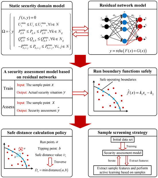
Figure 1.
Data-driven security operation assessment policy diagram.
Firstly, according to the concept of the safe operation boundary of the power system, combined with the characteristics of the residual network model, the mapping relationship between input and output characteristics is obtained, and the safety operation evaluation model based on the residual network is established. According to the safety operation evaluation model, the security boundary function of the large power grid based on the residual network is sorted out. A safety distance estimation strategy is constructed based on the safe operation boundary, and the actual operating status of the power system operation point is quantified to improve the mastery of power system operation status. At the same time, an active learning strategy is set for the model, enabling it to iteratively train on the sample set step by step, reducing the impact of errors in the sample set, and iteratively training the safety operation evaluation model based on the optimized training set to improve its accuracy.
2.1. Boundary Model of Safe Operation of Power System
For the power system under steady-state conditions, in order to ensure good power quality, the voltage magnitude at each node must be maintained within a certain range [20]. Assuming that the voltage magnitude at node is , the constraint on the voltage magnitudes of the power system can be expressed as Equation (1),
where and represent the upper and lower limits of the voltage amplitude of node , respectively. is the total number of nodes.
In order to avoid the problem of system instability caused by overload of equipment, line heating, and other reasons, the current of each branch of the power system is often required to be kept within a certain range, and the current constraint of the branch of the power system can be expressed as Equation (2),
where represents the current amplitude of branch ; represents the maximum constraint value of the current amplitude of branch .
As the equipment responsible for the injection of active and reactive power of the power system, the input capacity of the active and reactive power of the generator also needs to be limited due to the stability of the power grid and voltage, the overload protection of the generator itself, the reactive power compensation, and other reasons [21]; the active capacity constraint and reactive capacity constraint of the power system generator are shown in Equation (3),
where and represent the active and reactive power output of generator , respectively; and represent the lower limits of active and reactive power output of generator , respectively; and represent the upper limits of active and reactive power output of generator , respectively.
Combining the above constraints, assuming that the power grid has node and the set of generator working units is , the model of the safe operation boundary can be expressed as Equation (4), considering the constraints such as voltage limiting, generator set output constraint, and power flow balance in the node power injection space:
where is the voltage vector of the node, and is the injected power vector of the node; is the power flow equation of the AC system, and and represent the upper and lower limits of the voltage amplitude of node , respectively. and represent the upper and lower limits of the active output of generator , respectively; and represent the upper and lower limits of the reactive power output of generator , respectively; and are the bidirectional transmission limits of the active power for branch , respectively.
2.2. Residual Network Model
In view of the shortcomings of traditional neural network models, the residual network is optimized for its degradation problem, and a direct edge/short connection strategy is added, which effectively solves the problems of gradient disappearance and explosion. As a special form of neural network, it also includes an input layer, a hidden layer, and an output layer. The structure of residual blocks and jump connections is introduced, and each residual block contains a convolutional layer for feature extraction and a jump connection for residual learning. The jump connection in the residual network adds the input directly to the output to create a residual map, which can make the gradient propagate backwards, avoid network degradation through identity mapping, and alleviate the gradient disappearance and degradation problem of the neural network [22], as shown in Figure 2.
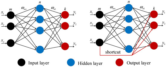
Figure 2.
Comparison of neural network and residual network principle model.
In the residual network, by setting the residual blocks and connecting them, the next layer can be made with more information, thereby improving the performance of the model, and its structure is shown in Figure 3. The whole residual block consists of two parts: the identity mapping part and the residual part. Among them, the identity mapping part is the most obvious distinguishing feature between the residual network and other neural networks, which directly adds the input to the output of the residual part, obtaining the final output result [23].
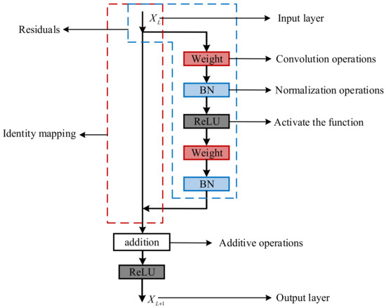
Figure 3.
Structure diagram of the residual block algorithm.
With the addition of identity mapping, the output changes from to , and the residual network can solve the phenomenon of gradient vanishing in the deep network, which can be explained by Equation (5),
This equation represents the identity mapping of the network from layer to layer , where is the input of layer in the network; is the input of layer in the network, and in the process of backpropagation, the derivative of the gradient formula can be obtained in the form of Equation (6),
From the above equation, it can be seen that the gradient of backpropagation in the residual network consists of two items, one of which is the identity mapping of , and its gradient is one after derivation. Due to the existence of this term, when the gradient of the multi-layer network degenerates to zero, there will be no gradient disappearance, and the idea diagram of the overall residual network model is shown in Figure 4. The overall model includes convolutional layers, pooling layers, residual modules, and fully connected layers. The classification results can be output as probabilities after processing by the fully connected layer.
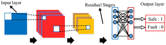
Figure 4.
Residual network model feature extraction diagram.
The structure of the residual block algorithm according to Figure 3: The convolutional layer can extract the local features of the input data information. The batch normalization layer can normalize the inputs of each layer to make the data distribution stable. Activating layers can increase the nonlinear representation of the model. The residual network can be modeled as follows in Equation (7),
where is the residual function; is the identity mapping function. After adding the two, the final output of the residual network model is obtained through the activation function.
In order to realize the combination of the residual network model and the boundary model of the safe operation of the power system, the inputs and outputs of the overall model are selected. The sample dataset is obtained under a fixed power system topology, and for the data of a certain operating point, it contains the information of the active power, reactive power, voltage, branch current, and power system safety of the nodes under the sample point. Therefore, this paper takes the active power of the node and the security information of the power system as the input of the training residual network model, and trains the residual network model. After obtaining the security operation evaluation model, the node active power is used as the input of the model and the security assessment result is used as the output to construct the security operation evaluation model framework based on the residual network, as shown in Figure 5.
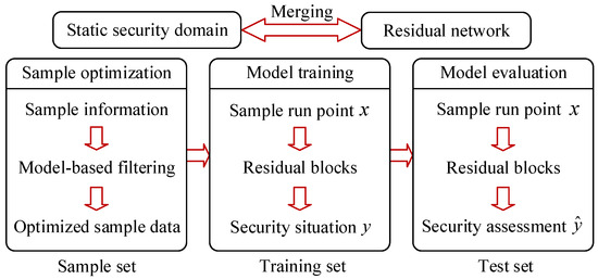
Figure 5.
Idea diagram of security operation evaluation based on residual network.
The sample set is divided into training set and validation set, and the model is trained through the training set to realize the active learning and iteration of the model to the sample set, so as to improve the accuracy of the model.
2.3. A Security Boundary Construction Method Based on Residual Network
According to the residual block structure, the basic mathematical expression of the residual block can be expressed as shown in Equation (8) below.
where is the input and output of the -layer residual block, respectively; is the influence coefficient of convolution and normalization in the residual block; is the activation function, which realizes the extraction of features and enhances the expression ability of features.
Let the initial sample training set be , where is the input of the model, which represents the operation of the power system, including the injected active power of each running node; is the actual operation of the power system. By setting the number of residual blocks to , all of which are fully connected in a single layer, the residual block model based on the residual network can be represented as shown in Equation (9),
where is the output of residual blocks; are the parameters of the first convolutional layer and batch normalization layer of the residual part of each residual block; are the parameters of the second convolutional layer and the batch normalization layer for the residual portion of each residual block [4].
In the field of machine learning, in order to make the classification independent of each other, the model output is generally set by one-hot encoding. Since the output is categorized as safe and unsafe, you can set them to and , respectively. Sorting out Equation (9) yields the classification information as shown in Equation (10),
where is the classification probability information after the output of the residual block processed by the fully connected layer, which contains the prediction probability of safety and insecurity. is the model parameter in the fully connected layer.
From Equations (9) and (10), it can be seen that the residual network model is trained with the power system operation point case as the input, the actual safety situation of the power system as the output, and and as the training set. Finally, the prediction of the safe operation of the power system is realized, which means the operation of the actual operation point of a power system can be input to obtain the prediction probability of safety and insecurity after the classification layer processing, and the two probabilities of safety and insecurity are included in the prediction probability , and the safety assessment results of the power system are obtained according to the size of the two. The boundary function for the safe operation of a large power grid based on the residual network can be expressed as follows in Equation (11),
where is the parameter after the dimensionality reduction in the parameters of the fully connected layer. Since the function is an implicit function, subsequent selection of support vector points is performed to represent the boundary function using the support vector machine algorithm [4].
3. Safety Margin Estimation Strategy Based on Safe Operating Boundary Function
3.1. Safe Distance Model
The safety distance refers to the Europa distance from the operating point to the safe operating boundary. Although the safety operation boundary may be a high-dimensional, nonlinear complex model, according to the definition of the safe operation boundary, it is a two-dimensional model and will not be affected by the increase in the dimensionality of the security domain [24]. Therefore, in the face of large-scale power systems with many nodes, the safety problems of operation analysis with safe distances are still applicable. According to its definition, the safe distance can be expressed as follows in Equation (12),
where is the point on the safe operating boundary; is the power situation of the running point; is a safe operating boundary. The safety distance can be described as the distance between the operating point and a certain point on the boundary, and its numerical magnitude indicates the safety situation of the operating point. The safety distance depicted in this paper can be expressed as Equation (13) in two-dimensional space; and the expression of Equation (12) can be expressed as follows:
where is the point on the safe operation boundary; is the power of the running point; the safe distance is the distance between two points.
3.2. Safety Margin Estimation Strategy
To facilitate visual analysis, a schematic diagram of the safe distance has been drawn, as shown in Figure 6. It can be seen that when determining the safe operating boundary of the large power grid, regardless of whether the shape of the safe operating boundary is regular, there is always a point on the boundary that has the shortest distance to a certain operating point within the safe operating boundary, and this distance is the estimated safety margin for that point.
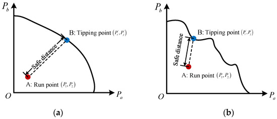
Figure 6.
Schematic diagram of the safety distance: (a) safe operating boundaries of the rules. (b) Irregular safety operation boundary.
The safe distance can be calculated according to Equation (13). For a safe operation point , the shortest distance from the boundary of the point is generally taken as the safety margin of the point, and the formula is shown in Equation (14),
where is the operation point where the safety margin is to be required; is the point on the safe operation boundary. The flow chart is shown in Figure 7.
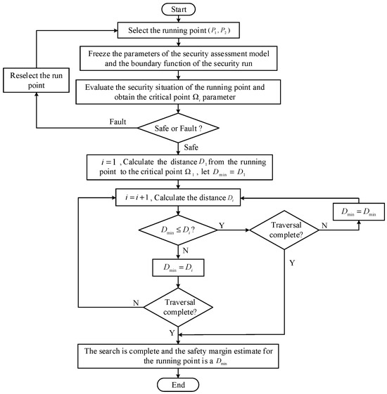
Figure 7.
Flow chart of the safety margin estimation strategy.
4. System Examples and Result Analysis
4.1. Overview of the Node System
In this paper, the three-machine nine-node system is used to verify the effectiveness of the proposed method, and the security operation evaluation model based on the residual network, the security boundary construction method based on the security evaluation model, and the security margin estimation strategy based on the security boundary are simulated and verified; and the three-machine nine-node system diagram is shown in Figure 8. The system consists of three generators and nine nodes, with each representing a busbar connected by transmission lines and transformers, forming a typical power system network structure [25,26,27].
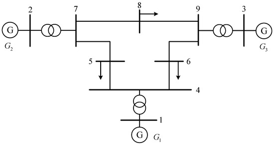
Figure 8.
IEEE9 node system diagram.
The system consists of PQ nodes, PV nodes, and balance nodes, of which PQ nodes occupy most of the nodes, and PV nodes occupy a small part of the nodes; there is only one balance node. In the system parameter setting in this paper, using the node system model in MATLAB/MATPOWER (7.1), the PQ node is node 4~9, which can consume a certain amount of active and reactive power. The PV nodes are nodes 2 and 3, which can control the active power and voltage amplitude output by the generator. The balance node is node 1, which can provide the overall reference voltage angle of the system and balance the active power, playing a role in maintaining the power balance of the system.
4.2. Sample Data Generation
In this paper, the sample training set data is generated by adjusting the power generation power of the generator node; that is, by changing the injection power of the generator node, the classification label of the system operation is either safe or unsafe, which is used to train the subsequent residual network model. Since the generator node 1 belongs to the balance node in the system, the active output of generator 2 and generator 3 is adjusted, and the active output of the balance node 1 is obtained through the power flow calculation, and a set of input vector can be obtained by adjusting the combined output multiple times. The flow chart of generating the sample training set is shown in Figure 9.
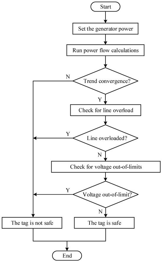
Figure 9.
Flow chart of sample training set generation.
To test the actual safety of the system for each combination of input vectors, this paper conducts safety verification of generator output constraints, node voltage constraints, and DC current constraints, respectively. First, check whether the actual output of each generator node exceeds the limits. As the output of the balancing node is obtained through power flow calculations, limit exceedance may occur. Next, check whether the voltage amplitude of each node is within the constraint range. Finally, check whether the branch current exceeds the limits. An operating point that meets all three conditions is a safe and stable operating point, formatted as ; if any of the conditions are not met, it is deemed an unsafe operating point, formatted as . According to the specified strategy from the above samples, output fluctuations are set for the generator nodes in a three-machine nine-node system to form generator combinations under different output conditions, thus generating a series of sample datasets.
A total of 1054 data samples were generated in this paper, and the data of the generated sample training set were visualized and plotted in Figure 10 and Figure 11 below. As shown in Figure 10a, the two-dimensional visualization map mapped to the P2 and P3 nodes, whereby the green dots represent the data points that can meet the safe operation conditions, and the red dots represent the data points that cannot meet the safe operation conditions. When the injection power of P2 and P3 is too large or too small, the safe and stable operation of the power system cannot be guaranteed. Only a combination of injected power in an area can achieve safe and stable operation of the system. Under the constraint of power flow equilibrium, considering the safe operating conditions of all aspects of the power system, the injection power of generator P2 and P3 can be adjusted to obtain the injection power of generator P1, so as to form the injection power vector of generator set. Under the injection power vector of each sample, the safety analysis of the power system can obtain the three-dimensional visualization of the sample training set in Figure 10b.
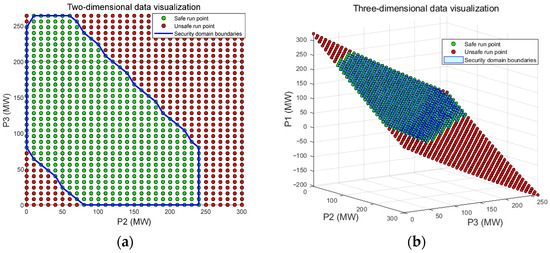
Figure 10.
Visualization of the sample training set: (a) two-dimensional sample data visualization diagram; (b) three-dimensional sample data visualization diagram.
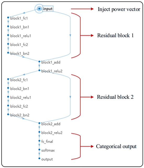
Figure 11.
Training diagram of the residual network model.
According to the output combination settings of the above generators, a sample dataset is generated, and the data of some sample training sets are shown in Table 1 below. For example, using samples 2 and 3, in sample 2, the output of generator p1 is 313.6 MW; the output of generator p2 is 10 MW; and the output of generator p3 is 0 MW. Under this generator set output combination, the power system is in an unsafe operating state, meaning the safety label is 0. In sample 3, the output of generator p1 is 243.5 MW; the output of generator p2 is 20 MW; and the output of generator p3 is 56 MW. Under this generator set output combination, the power system is in a safe operating state, meaning the safety label is 1.

Table 1.
Some sample training set data.
4.3. Simulation Analysis of the Case
4.3.1. A Security Operation Evaluation Model Based on Residual Networks
According to the sample training set data generated above, the residual network model proposed in this paper is trained, and the training diagram of the residual network model is shown in Figure 11.
According to the model framework defined for the model, when the model is trained, the two-dimensional injected power vector and safety label of the sample training set are , where means that the power system cannot achieve safe and stable operation under the power vector, and means that the power system can achieve safe and stable operation under the power vector. After the data processing and feature extraction of the two residual blocks, the mapping relationship between the two-dimensional injection power vector and the safety situation label can be obtained, and the mapping relationship can be realized: under a fixed power system topology, when a two-dimensional injection power vector is input, a system safety situation under the vector can be output, and the evaluation of the safe operation of the power system can be realized.
In this paper, the generated 1054 data samples are divided into 70% training set and 30% validation set; the model is trained through the training set and the accuracy of the model is verified through the validation set. The ResNet structure set in this paper has 21 layers; the optimizer chosen is the Adam optimizer, which is suitable for most deep learning tasks. The training is conducted for 100 epochs, with a mini-batch size of 64, a validation frequency of 30, an initial learning rate set to 0.001, and a learning rate decay factor of 0.5.
Through iterative training of the model, each model is based on the previous one, serving as the foundational model for the next model’s iterative training. The sample training set is gradually iterated and screened to extract the features of the sample set. The iterative effect of the security operation evaluation model shown in Figure 12 below can be obtained. Figure 12a is a rendering of the safety assessment model for one round of iteration of the assessment model, with 30 iterations in each round, for a total of 30 iterations; Figure 12b shows the effect diagram of the safety assessment model for five iterations of the assessment model. The model has 30 iterations in each round, with a total of 150 iterations. Figure 12c is a rendering of the safety assessment model for 10 iterations of the assessment model, with 30 iterations in each round, with a total of 300 iterations; Figure 12d shows the rendering of the security assessment model for 20 iterations of the assessment model, with 30 iterations in each round, for a total of 600 iterations. It can be seen that with the increase in the number of iterations, the model grasps more and more features of the training set data, and the security operation boundary depicted is more and more in line with the actual security boundary.
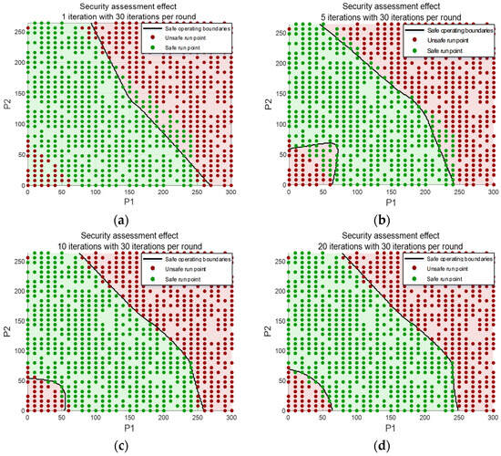
Figure 12.
Iterative rendering of the security assessment model: (a) a total of 30 iterations; (b) a total of 150 iterations; (c) a total of 300 iterations; (d) a total of 600 iterations.
The accuracy of the evaluation model is verified using the validation set. As the number of iterations increases, the iterative process is illustrated in Figure 13. During model training, the number of training epochs was set to 100, with 130 iterations per epoch. In Figure 13, the horizontal axis represents the number of iterations, and the vertical axis represents the accuracy. When the model goes through only one iteration on the training set data, the accuracy on the validation set is only 42.38%, indicating that the evaluation model cannot fully capture the characteristics of the training set. When the number of iterations reaches 90, the accuracy on the validation set reaches 90.00%. As the number of iterations increases, the overall validation accuracy shows an upward trend, but the rate of accuracy improvement slows down. When the number of iterations reaches 1300, the validation accuracy can reach 99.57%.
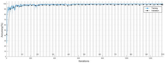
Figure 13.
Flow chart of iteration accuracy.
4.3.2. Security Boundary Construction Based on Security Assessment Model
When the number of iterations is 1300, the accuracy of the validation set reaches 98.57%, and the evaluation model is used as the benchmark for constructing the boundary function of the safe operation, and the evaluation effect of the security model is shown in Figure 14. It can be seen that the evaluation model can obtain the characteristics of the training set very accurately and can effectively depict the actual location of the security operation boundary.
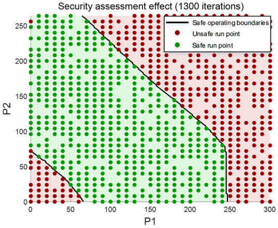
Figure 14.
Final rendering of the safety assessment model.
Since the residual network model is a black-box model, the boundary function represented by function expressions is fuzzy. In this paper, combined with the SVM support vector machine algorithm, the security operation boundary function based on the residual network model is expressed, and the residual network decision boundary is fitted. Use the prediction results of the residual network as new labels to train an SVM model to approximate the decision boundary of the residual network, extract the key points of the boundary as support vectors, and set the kernel function of the SVM to a polynomial kernel function, which is highly adaptable to safety boundaries in two-dimensional visualization. The safe operation boundary function based on the residual network model can be expressed as Equation (15).
In the equation, is the input parameter vector; is the support vector, which is the boundary key point; and are the importance weights of the support vectors; is the decision boundary offset. Expanding the equation yields the boundary function expression shown in Equation (16), and Figure 15 shows the security boundary diagram and key boundary points obtained through the SVM algorithm.
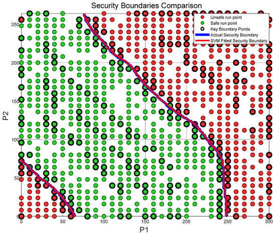
Figure 15.
Fitting effect diagram of safe operation boundary based on SVM algorithm.
4.3.3. Security Margin Estimation Based on Security Boundaries
Based on the above safety operation evaluation model and safety operation boundary, this paper estimates the safety margin of seven safety operation points of , calculates the Euclidean distance between each point and the critical operation point, and selects the minimum distance as the safety margin of the point, which can be represented by the safety margin estimation strategy of the seven safety operation instance points as shown in Figure 16 below.
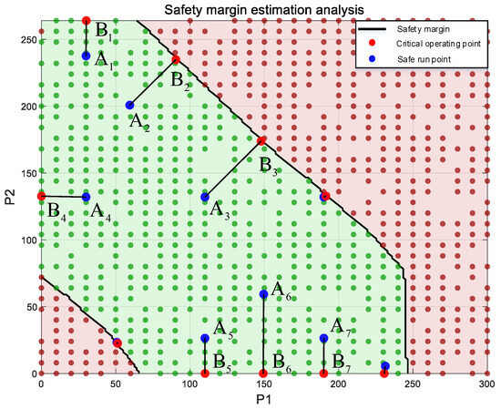
Figure 16.
Safety margin estimation diagram under different system operating points.
Through visual analysis, the larger the distance between the safe operation point and the critical operation point, the larger the estimated safety margin of the point, and the safer the safe operation point. The detailed coordinates and safety margin of each point are displayed in Table 2. For the safety margin, the estimated magnitude can be understood as the maximum injection power value that can be changed by the generator, and by quantifying the safety margin, the mastery of the operating point can be improved [28,29,30].
Table 2.
Estimation of safety margin at operating point.
5. Conclusions
This article, based on a machine learning model driven jointly by data and models, achieves accurate assessment of the safe operation of power systems, and to some extent enhances relevant personnel’s understanding of the safety and stability of power systems. This paper considers leveraging the data processing advantages of machine learning models in the assessment of power system safe operation, and establishes a safe operation evaluation model based on a residual network. On this basis, a method for constructing the safe operation boundary of a large power grid based on the residual network is proposed, and an estimation strategy for safety margins is suggested accordingly. Taking the IEEE nine-bus system as an example for case verification, simulation results show the following:
- (a)
- This paper uses the IEEE nine-bus system for simulation examples. The system has a simple yet complete structure and can clearly demonstrate the construction effects in the visualization of secure operation boundaries, showing strong adaptability in constructing secure operation boundaries.
- (b)
- The proposed residual network model can accurately capture the mapping relationship between generator injection power and power system security. By evaluating the model to select sample training sets, it can effectively improve the model’s training performance and enhance prediction accuracy for the safe operation of the power system. When determining secure operating boundaries, integrating it with the SVM model effectively addresses the black-box problem of the residual network, reduces model complexity, and improves adaptability across different scenarios.
- (c)
- The proposed safety margin estimation strategy can quantify the safety degree of the power system operation point and improve the operator’s grasp of power system operation.
The active learning strategy proposed in this paper has a strong dependence on the initial model, and the addition of a certain limitation strategy is considered for the subsequent model to reduce dependence on the initial evaluation model. This has led to more effective iterative strategies, which is an issue that needs further investigation.
Author Contributions
H.D.: responsible for resources, formal analysis, program compilation, and writing—original draft. C.X.: responsible for writing—review and editing. W.M.: responsible for methodology and project administration. N.Z.: responsible for obtaining the experimental data. X.W.: responsible for investigation and resources. F.X.: responsible for funding acquisition and resources. All authors have read and agreed to the published version of the manuscript.
Funding
This research work was supported by the Science and Technology Project of State Grid Corporation of China Headquarters titled “Research on Full-Cycle Analysis and Emergency Support Technology for Unconventional Events in Large Power Grids” (Topic 2: Research on Emergency Technology for Collaborative Dispatching of Source-Grid-Load Resources to Cope with Strong Impacts of Unconventional Events, Project No.: 5100-202416027A-1-1-ZN).
Data Availability Statement
Data is contained within the article.
Conflicts of Interest
Authors Hongxiang Dong and Chuanliang Xiao are employed by Shandong University of Technology. Author Weiwei Miao is employed by State Grid Shandong Electric Power Company. Authors Ning Zhou, Xinyu Wei, and Facai Xing are employed by Electric Power Research Institute of State Grid Shandong Electric Power Company. The remaining authors declare that no commercial or financial relationships that could be construed as a potential conflict of interest existed during the conduct of this research.
References
- Chen, X.; Zhang, G.; Zhang, C.; Chen, J.; Guan, J.; Liu, Z. Research on strategies for enhancing the security resilience of new power systems empowered by digital technology. China Eng. Sci. 2025, 27, 168–179. (In Chinese) [Google Scholar] [CrossRef]
- Fan, S.; Zhao, Z.; Guo, J.; Ma, S.; Wang, T.; Li, D. Overview of Data-Driven Assessment Methods for Transient Stability of Power Systems. Proc. CSEE 2024, 44, 3408–3429. (In Chinese) [Google Scholar] [CrossRef]
- Mu, T.; Liu, S.; Yang, Z.; Guo, Y.; Zhang, A.; Liu, Z. Rapid Calculation of Transient Voltage Safety Domain in Scenarios with Variable Topological Parameters. J. Electr. Power Syst. Autom. 2024, 36, 126–131. (In Chinese) [Google Scholar] [CrossRef]
- Chen, Y.; Lu, C.; Liu, D.; He, J. Safety assessment and safety margin estimation of transient voltage based on active learning in multi-fault scenarios. J. Wuhan Univ. 2023, 56, 1336–1346. (In Chinese) [Google Scholar] [CrossRef]
- Ji, K.; Qiao, J.; Zhao, Z.; Zhao, J.; Shi, M.; Yang, F. Adaptive Assessment of Transient Stability of Power Systems Considering Uneven Sample Distribution. Power Syst. Technol. 2025, 49, 1–13. (In Chinese) [Google Scholar] [CrossRef]
- Wang, B.; Pi, J.; Wang, X.; Qi, X.; Sun, W.; Huang, Q.; Wei, C.; Zhang, X.; Xu, X.; Wang, Z. A rapid assessment method for supply and demand imbalance risk in a new power system based on deep active learning driven by weather data. Power Syst. Technol. 2024, 48, 4050–4060. (In Chinese) [Google Scholar] [CrossRef]
- Cai, M.; Fan, R.; Wang, H.; Cui, M.; Li, Y.; Cheng, H. Research on a topology reconstruction method for three-phase unbalanced distribution systems based on data-driven recursive AdaBoost. Smart Power 2025, 53, 38–44. (In Chinese) [Google Scholar] [CrossRef]
- Lin, W.; Li, X.; Zhou, R.; Zhu, Y.; Peng, Y. Low-carbon optimization operation method of microgrid based on deep reinforcement learning. Mod. Electr. Power. Available online: https://kns.cnki.net/kcms2/article/abstract?v=ZHE1803t14uUeK-KZShPdidwIZ6V1FFVeE_XniEfOynxfGSA-QfNkqk3YwT36_U59McwuNiplVWLVI7R2fNCfwmeQ5v4dtK2Ib_CdmWCLlw7MKROGYvTsZK9IqU3W4JXKELQtybg_B5Wod0l-eK0FyPSC2AfTBqgM_3x6hAQ364=&uniplatform=NZKPT&language=CHS (accessed on 2 November 2025). (In Chinese).
- Duan, S.; Yu, J.; Yang, Z.; Chen, T.; Zhu, S. Intelligent adjustment method of power grid operation mode based on N/N-1 power flow embedded graph convolutional neural network. J. Electr. Eng. Technol. 2025, 40, 1–15. (In Chinese) [Google Scholar] [CrossRef]
- Wang, L.; Zhou, Y.; Zhang, Y.; Li, Y.; Ai, H. Fusion identification method of weak points in the power grid based on RMT. South. Power Grid Technol. Available online: http://kns.cnki.net/kcms/detail/44.1643.tk.20250422.1633.026.html (accessed on 2 November 2025). (In Chinese).
- Liu, S.; Dang, X.; Cui, Z.; Yang, C.; Yuan, Z.; Yuan, M. A method for transient stability assessment of power systems using deep residual networks for sample class imbalance. Smart Power 2024, 52, 116–123. (In Chinese) [Google Scholar] [CrossRef]
- Chen, K.; Wang, Z.; Guo, Y. Evaluation of Transient Voltage Stability of a Wind Power Grid-Connected System Based on the grcForest Model. Smart Power 2023, 51, 31–37. (In Chinese) [Google Scholar] [CrossRef]
- Wang, J.; Zheng, F.; Zhang, P.; Chen, L.; Gao, H.; Meng, J. Planning model of high-proportion renewable energy distribution network based on data-driven. Electr. Power 2025, 58, 175–182. (In Chinese) [Google Scholar] [CrossRef]
- Cui, X.; Zhao, J.; Zeng, Z. A data-driven prediction method for nodal frequency based on spatiotemporal distribution characteristics. J. Shanghai Electr. Power Univ. 2025, 41, 231–236. Available online: http://kns.cnki.net/kcms/detail/31.2175.TM.20250427.1354.004.html (accessed on 2 November 2025). (In Chinese).
- Xiang, D.; Wang, B.; Guo, W.; Chu, X.; Yu, Z. Refined Safety Operation Rules for Power Systems Based on Artificial Neural Networks. Power Syst. Prot. Control 2017, 45, 32–37. (In Chinese) [Google Scholar] [CrossRef]
- Zhu, P. Research on Static Safety Assessment Methods of Power Systems Based on CNN. Autom. Instrum. 2025, 46, 70–74. (In Chinese) [Google Scholar] [CrossRef]
- Teng, W.; Mei, Q.; Zhao, Y. Short-term power load prediction method based on improved residual network and BiGRU. Co. Eng. Available online: https://link.cnki.net/urlid/21.1476.tp.20241125.1354.004 (accessed on 2 November 2025). (In Chinese).
- Zhang, J.; Qiu, J.; Zhu, Y.; Zhu, Y.; Yang, H.; Xu, G.; Tu, L. Security and stability control method of new energy grid based on temporal convolutional residual network and pelican optimization algorithm. Renew. Energy 2024, 42, 845–852. (In Chinese) [Google Scholar] [CrossRef]
- Chen, S.; Liu, P.; Wang, P.; Ma, J. Load forecasting method for power systems based on LSTM artificial neural networks. J. Shenyang Univ. Technol. 2024, 46, 66–71. (In Chinese) [Google Scholar] [CrossRef]
- Li, L.; Wu, J.; Li, B.; Wang, Y.; Wang, C.; Dong, X. Two-stage multi-level early warning of frequency safety in power systems based on improved residual network. Autom. Electr. Power Syst. 2023, 47, 22–34. (In Chinese) [Google Scholar] [CrossRef]
- Zhao, J.; Qiu, L.; Huang, H.; Jia, H.; Li, P.; Li, Z. Boundary characteristics of thermal stability safety domains in multidimensional space fault surfaces. Power Syst. Autom. 2014, 38, 39–45. (In Chinese) [Google Scholar] [CrossRef]
- Xie, W.; Shen, J.; Zhang, Q.; Zhu, S.; Wang, N. Transient Voltage Stability Evaluation Algorithm for High Voltage DC Receiver Power Grid Based on FCM Clustering and Deep Residual Network. South China Electr. Power Technol. Available online: https://link.cnki.net/urlid/44.1643.TK.20250603.1534.008 (accessed on 2 November 2025). (In Chinese).
- Kuang, Q.; Li, J.; Bai, S. SSO Modal Parameter Identification Based on Deep Residual Network. Electron. Meas. Technol. 2022, 45, 57–63. (In Chinese) [Google Scholar] [CrossRef]
- Liu, Y.; Gu, X.; Wang, T. Optimal Dispatching of Wind Power Grid Safety Considering Static Safety Distance. Power Syst. Prot. Control 2021, 49, 93–99. (In Chinese) [Google Scholar] [CrossRef]
- Yang, Y.; Pan, F.; Zhong, L.; Zhang, J.; Zhao, J.M. Prediction Method of Carbon Emission Factors at Power System Nodes Based on Neural Network. Guangdong Electr. Power 2023, 36, 2–9. (In Chinese) [Google Scholar]
- Zhao, Z.; Peng, K.; Xian, R.; Zhang, X. Localization of Oscillation Source in DC Distribution Network Based on Power Spectral Density. J. Mod. Power Syst. Clean Energy 2023, 11, 156–167. [Google Scholar] [CrossRef]
- Wang, W.; Feng, C.; Guan, Y.; Ma, W.; Che, L. A Hybrid Modeling and Simulation Driven Method for Rapid Unit Commitment Solving Aimed at Reliability Improvement. Autom. Electr. Power Syst. Available online: https://link.cnki.net/urlid/32.1180.TP.20250929.2155.006 (accessed on 30 October 2025). (In Chinese).
- Fan, M.; Zhang, S.; Dai, F.; Zheng, H.; Zhang, X.; Liu, Z.; Jing, Z. A Rapid Multi-Value Assessment Method for Power Systems Based on VCG Mechanism and State Space Compression. China Electr. Power. Available online: https://link.cnki.net/urlid/11.3265.TM.20251029.1026.002 (accessed on 30 October 2025). (In Chinese).
- Liu, B.; Li, Z.; Hu, J.; Yu, S.; Li, W. Method to enhance the operational adequacy of the receiving-end power grid considering the relaxation of static voltage security boundaries. High Volt. Technol. Available online: https://link.cnki.net/urlid/42.1239.tm.20250919.1333.005 (accessed on 2 November 2025). (In Chinese).
- Zhai, S.; Zhang, Y.; Lu, X.; Huang, W.; Zheng, C.; Wei, S.; Yao, W. Intelligent Assessment of Power System Frequency Security Based on Global Feature Embedded Graph Attention Network under Anticipated Faults. South. Power Grid Technol. 1–12. Available online: https://link.cnki.net/urlid/44.1643.TK.20251009.0907.008 (accessed on 30 October 2025). (In Chinese).
Disclaimer/Publisher’s Note: The statements, opinions and data contained in all publications are solely those of the individual author(s) and contributor(s) and not of MDPI and/or the editor(s). MDPI and/or the editor(s) disclaim responsibility for any injury to people or property resulting from any ideas, methods, instructions or products referred to in the content. |
© 2025 by the authors. Licensee MDPI, Basel, Switzerland. This article is an open access article distributed under the terms and conditions of the Creative Commons Attribution (CC BY) license (https://creativecommons.org/licenses/by/4.0/).