Abstract
This study addresses developing systematic guidelines for the design of concentration control in the oxidation of benzene to maleic anhydride within a tubular reactor. The influence of step size selection and temperature sensor location on the tuning and performance of a PI/P cascade control system applied to the oxidation process was evaluated. The reactor’s dynamic behavior was analyzed using numerical simulations based on the solution of the Fortran mathematical model. Sensor positions and multiple step sizes (from +10% to −10%) were analyzed to characterize reactor dynamics and optimize control parameters. The results show that a controller design corresponding to a −9% step in the jacket temperature offered the best performance, ensuring process stability and selectivity. In contrast, step changes between +10% and −8% caused temperature deviations beyond safe limits. Since maleic anhydride is an essential precursor in the production of resins, plastics, lubricants, and pharmaceutical intermediates, optimizing the efficiency and safety of its production represents a significant benefit to the global chemical industry.
1. Introduction
Growing industrial demand has driven the continuous updating of processes in order to make them more efficient and at the same time, more sustainable. Technologies that are vital for complex processes today were considered an option in earlier decades, such as process control, which the Greeks had an idea of as early as 300 BC, when they began to design feedback systems to correct the water level, using a system similar to the float valve in today’s toilets. Later, around 1681, Denis Papin invented the safety valve in order to control steam pressure, creating what we know today as the pressure cooker. On the other hand, Cornelis Debbel in Holland invented a mechanical system to control the temperature when incubating eggs [1].
By the 20th century, discoveries in the control area, such as those made by Bode, Hazen, Nichols, Nyquist, among many other researchers, were able to establish key principles, tools and methods that are still valid today for process control [2]. Finally, the Internet of Things (IoT) presented a significant opportunity in the development of more efficient and adaptive control systems [3].
Advances in control engineering, from the first mechanical controllers to more sophisticated automatic controls, have culminated in modern control theory, which has simplified the design of control systems based on models of the real system consisting of the use of differential equations. In recent years, control research has moved towards adaptive and intelligent strategies capable of dealing with nonlinearity, uncertainty, and dynamic constraints of systems. For example, Cheng et al., 2025 [4] proposed a nonlinear adaptive control method with active disturbance rejection for distributed generation systems based on high-speed permanent magnet synchronous generators, achieving higher robustness and faster convergence. Similarly, Zhang et al., 2023 [5] developed an adaptive control scheme based on fuzzy logic and barrier-type Lyapunov functions (BLF) applied to intelligent actuators with hysteresis, managing to keep all system variables within established limits and guaranteeing stability. For their part, Li et al., 2025 [6] introduced an active disturbance rejection control method using Actor-Critic Enhanced Reinforcement Learning applied to electrohydrostatic actuators, demonstrating effective disturbance compensation, parameter self-tuning capability, and convergence without prior knowledge of the system. These studies reflect a growing trend toward the integration of artificial intelligence, adaptive algorithms, and nonlinear control theory with the aim of improving system robustness and performance in complex and time-varying environments.
While adaptive and intelligent control strategies dominate current research, cascade control remains a widely used structure in process industries due to its simplicity, robustness, and ability to efficiently handle disturbances. Recent studies demonstrate growing interest in cascade control applications across various industrial systems, including tubular reactors, oxidation processes, and thermal and electromechanical systems. However, most of these works focus mainly on control efficiency under external disturbances, generally employing a single step change for controller design and tuning. This conventional approach limits the understanding of dynamic behavior by neglecting how step magnitude or sensor location influences process characterization, controller design, thermal stability, selectivity, and overall process yield.
The oxidation reaction to obtain maleic anhydride has been produced for 150 years and is considered of great commercial importance; after acetic and phthalic anhydride, it is one of the most important commercial anhydrides in use [7].
The industrial production of maleic anhydride is a key precursor in the manufacture of many products. Maleic anhydride is used in the formulation of hair, skin, and oral care products [8]. On the other hand, it also forms part of pharmaceutical and biological components. The use of maleic anhydride in coating technology is also widespread. From the manufacture of automotive and architectural coatings to antimicrobial and antiadhesive coatings. Active compounds for the polymer industry, for the manufacture of resins, thermoplastics and films [9]. In this type of process, temperature and concentration control are essential to maintain the equipment in optimal operating conditions, thus minimizing the risk of producing unnecessary products due to the multiplicity of the reaction.
This study advances the understanding of nonlinear behavior in tubular reactors with multiple exothermic reactions by quantifying how step size characterization and sensor placement affect cascade control tuning and control performance. Unlike previous studies mentioned above, which primarily propose cascade control structures and focus on evaluating their effectiveness against disturbances, the present work addresses a critical gap: the influence of step characterization and sensor location on control performance has not been systematically analyzed for the partial oxidation of benzene carried out in a tubular reactor. Moreover, prior research has not explored how the choice of control structure can mediate the trade-off between selectivity and yield a key aspect for linking control theory with the chemical behavior of the process.
The developed methodology provides a systematic framework to identify control configurations that minimize deviations and enhance product selectivity. In doing so, it bridges the gap between theoretical modeling and practical control design, enabling adaptation to other highly exothermic processes. Therefore, this work contributes not only to improving the thermal safety and efficiency of the benzene-to-maleic anhydride process but also to establishing reproducible design guidelines for concentration control in nonlinear chemical systems, explicitly correlating control strategies with chemical performance metrics.
2. Materials and Methods
2.1. Process Simulation
The present study was conducted through a rigorous simulation of the benzene oxidation to maleic anhydride process, using the Force 2.0 compiler and a Fortran-based model of a tubular reactor.
In addition to its industrial relevance, this case was selected as the focus of this study due to its nature as a complex system for control design and analysis. The oxidation of benzene to maleic anhydride is a highly exothermic reaction system, sensitive to temperature changes, and with a multiple reaction mechanism, in which several parallel and consecutive reactions can occur, giving rise to both desired products (maleic anhydride) and undesired products. This reaction multiplicity makes the process extremely sensitive to temperature deviations. Inadequate control can easily divert the reaction towards undesired pathways, decreasing selectivity and promoting the formation of low-value byproducts for the process. Therefore, this process constitutes an ideal benchmark for evaluating cascade control strategies aimed at improving stability, selectivity, and overall process safety.
The oxidation of benzene to maleic anhydride consists of three exothermic, irreversible gas-phase reactions shown in Equations (1)–(3) that take place on solid V2O5-MoO3-P2O5 catalyst particles [10].
The molar flow mass balances for benzene and maleic anhydride are outlined by Equations (4) and (5) and the heat balance are shown in Equations (6) and (7) and as a partial differential equations are discretized using the finite difference method, the resulting ordinary differential equations, are integrated using the 4/5-order Runge–Kutta method, the process balance were taken from the works of Urrea et al., (2015) [11].
The developed model is based on material and energy balances that describe the dynamics of a tubular reactor for the oxidation of benzene to maleic anhydride. The simulations were performed considering the model and operating conditions reported in the literature [11,12], which contain all the details of the process modeling. Since the reactor model is not the main focus of this project, only the control application portion will be discussed.
With the following initial conditions,
Tc (t,0) = 697 K, Ts (t,0) = 760 K, Tf (t,0) = 709 K, FMA (t,0) = 0 mol s−1, FB (t,0) = 0.00927 mol s−1, v (t,0) = 2.48 m s−1.
The simulation was designed to realistically capture the dynamic characteristics of the reactor, including transport phenomena and measurement delays, ensuring that sensor dynamics were implicitly represented. From a modeling standpoint, the tubular reactor was described by partial differential equations for mass and energy balances, dependent on axial position and including convection and dispersion terms. These equations inherently reproduce transport delays and variations in time constants along the reactor. The model was discretized using the finite difference method, yielding a system of coupled ordinary differential equations that capture the distributed and delayed dynamics of the process.
2.2. Process Characterization and Tuning of the Control System
Once the dynamic behavior of the process was represented, we continued with its characterization in order to design the selected control system.
The configuration of the control structure to be used is a cascade type control consisting of the primary loop as proportional control and the secondary loop as proportiona–integral control, as shown in Figure 1.
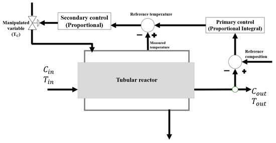
Figure 1.
Configuration of the Cascade Control Structure.
The proposed cascade control configuration is particularly suitable for scenarios in which the primary process variable cannot be measured directly or exhibits a significant time delay. In such cases, a secondary variable, readily measurable and dynamically correlated with the primary one, is employed as an intermediate control variable. By regulating this secondary signal, the system can exert an immediate and effective influence over the primary variable, enhancing overall control responsiveness.
In nonlinear and multi-reaction processes, where the dynamic behavior depends on several concurrent reactions, even small thermal disturbances can alter reaction rates, affect conversion levels, and modify product selectivity, ultimately leading to thermal instabilities or loss of process control. Under these conditions, the cascade control architecture provides a prompt corrective action to energy fluctuations before they propagate and adversely impact the main reaction, thus improving both process stability and operational safety.
In this process, cascade control provides precise and rapid compensation of disturbances affecting both reactor temperature and product concentration. The inner loop regulates the reactor temperature, while the outer loop maintains the desired product concentration, ensuring coordinated control of the system. This configuration mitigates the formation of hotspots and undesired by-products in highly exothermic, nonlinear reactions. Consequently, it enhances operational stability, selectivity, yield, and overall process safety.
The primary control will be responsible for regulating the output concentration of the reactor through which the maleic anhydride flows, the proportional part will adjust the variable to its required set point and the integral part will minimize the existing error while making the response faster, this external loop compares the concentration with the desired set point, generating a control signal based on the error in order to adjust the internal temperature of the reactor, formed a ratio of concentration over temperature.
On the other hand, the secondary control (proportional) will receive the signal from the primary control on the measurement of the internal temperature of the reactor and compare it with the desired value in order to adjust the jacket temperature to maintain the process at the proper temperature, relating the reactor temperature with the jacket temperature. The choice of proportional and proportional–integral (PI) controllers over more advanced strategies such as PID or model predictive control (MPC) was guided by practicality, reliability, and industrial applicability. Owing to their robustness, ease of tuning and maintenance, and long-standing validation in industry, PI controllers offer high operational confidence and adaptability without requiring complex models or computational tools.
The reference value of the reactor temperature is analyzed, considering different points along the reactor to take this measurement. Eleven temperature sensor locations were evaluated along the tubular reactor (5%, 10%, 20%, 30%, 40%, 40%, 50%, 60%, 70%, 80%, 90% and 95%), covering the inlet, outlet, hot spot, and several intermediate regions. This evaluation is essential because the tubular reactor exhibits significant temperature variations along its length due to the progress of the oxidation reactions, which modify the heat release and conversion profiles over time. Consequently, monitoring different axial positions allows capturing the thermal dynamics of the system more accurately and identifying the most representative point for feedback control. Furthermore, the inlet, outlet, and hot spot regions are often subject to higher instability, making sensor placement critical to ensure control robustness and process stability.
Once the sensor position has been defined, process characterization consists of implementing a pulse (step change) that allows measuring how the system variables (reactor temperature, jacket temperature, and concentrations) change over a period of time. Therefore, step sizes of (±10, 9, 8, 7, 6, 5, 4, 3, 2, and 1% in the jacket temperature) were implemented in the manipulated variable, the jacket temperature.
The step sizes were selected following the guidelines of Smith and Corripio (2014) [13], which ensures measurable responses and avoids nonlinear behavior that could distort the system dynamics. Excessively large step sizes can lead the system to unstable or highly nonlinear regions that are demonstrated in the process behavior, warranting that the choice of step size must be consistent with the model that represents the reality of the process, while excessively small steps produce imperceptible variations. Unlike most cascade control studies, which arbitrarily select step sizes to evaluate the response to perturbations, this work seeks to demonstrate that a carefully selected step size, combined with the strategic placement of sensors, can significantly improve the thermal stability and selectivity of the reaction.
To this end, the values of the response to the step change in the maleic anhydride composition and temperature are taken to calculate the gain (K), dead time (θ), and time constant (τ) parameters and build the approximation to a First-Order Plus Dead Time (FOPDTM) model. The proportional gains and the parameters mentioned above were determined using an empirical tuning procedure guided by the system’s dynamic response. Equation (8) is used for a step change in magnitude ∆m and a FOPDT model [13].
Since the concentration and temperature parameters are known, two functions are constructed for both parameters, where the gain (K) of the process is calculated as shown in Equation (9) [13]:
To obtain the values of dead time (θ) and time constant (τ), the response matching in the high rate of change region of the applied step change response is selected, and the values of θ and τ are obtained by solving Equations (10) and (11) [13]:
The design of the First-Order Plus Dead Time model considers the already calculated parameters of gain (K), dead time (θ), and the time constant (τ) for the composition and temperature at each of the 11 points selected along the reactor, whose transfer functions for composition and temperature are mentioned below [11].
For controller design, equivalent FOPDT models were fitted to the dynamic responses at each sensor location, effectively capturing transport and measurement delays through the parameters θ and τ. This modeling approach preserves a realistic representation of the reactor’s dynamic behavior while maintaining computational simplicity, thereby facilitating the development of practical and transferable control strategies for industrial applications.
The transfer function for composition is shown in Equation (12):
The transfer function for temperature is shown in Equation (13):
In the design of the primary loop, a relationship between the output composition transfer function and the temperature along each point of the reactor is established, as in Equation (14). Therefore, the resulting transfer function can be expressed as the quotient of the composition over temperature transfer functions, obtaining Equation (15):
where .
Performing the division of both transfer functions yields a positive time constant numerator (see Equation (16)) whose purpose is to cancel its terms () against a denominator () where both T0 and τ0 are positive and real, this cancellation is performed using the approximations of [14].
Through this process it is possible to determine the values of gain , dead time θ, and time constant τ. Using the previously calculated parameters, Equation (17) is used to determine the integral time of the primary loop, and Equation (18) can be implemented to calculate the gain of the proportional integral control [14].
As observed, the implementation of the step change in the manipulated variable, which for this case study will be the jacket temperature, is important in the characterization of the process since the cascade controller tuning is based on the FOPDT model parameters. In the following sections, it is analyzed how different sizes of step changes affect the performance of the control system.
2.3. Evaluation of the Control Structure
In order to determine which control structure designed from the different step changes applied is the one with the best performance, the control system was evaluated by implementing a series of disturbances in the feed composition and feed temperature, observing the responses of selectivity, yield, and the values of the Absolute Integral Error.
The three types of perturbations applied to the process to evaluate the control system were as follows:
Disturbance 1: 10% benzene composition at 50 s;
Disturbance 2: 10% feed temperature at 50 s;
Disturbance 3: 10% benzene composition at 50 s and −10% of the feed temperature at 100 s.
The composition and temperature disturbances were selected to represent typical process fluctuations. The chosen magnitudes (+10% in composition and +10 °C in temperature) correspond to common deviations reported in the literature [15,16].
The improvement in performance was evaluated using the Integral of Absolute Error (IAE), showing a consistent reduction across all test scenarios. In addition, the selectivity and yield parameters were monitored to determine which control strategy provided the best overall performance. The transient response of the controlled variables was also analyzed, confirming faster stabilization and reduced overshoot. These results collectively demonstrate the robustness and effectiveness of the proposed controller in mitigating process disturbances and enhancing overall process efficiency.
2.4. Fractal Analysis
To design the PI/P cascade control structure, three control parameters were required, as mentioned in the control system tuning section (proportional gain, integral gain, and integral time). To graphically visualize how the control parameters change depending on the selected step size and sensor position, three-dimensional surfaces (control parameter-step size-sensor position) were constructed. Fractal analysis of the graphs was then performed to quantify the geometric complexity of the control structure and identify the relationship between fractality and the control system performance achieved after implementing the disturbance sequences.
The fractal dimension was estimated using the 3D box counting method. To do this, the data were normalized to the range 0.01 and overlaid with cubic meshes of different sizes. At each scale, the number of occupied cubes was counted, constructing the relationship log(N(ϵ)) versus log(1/ϵ). The slope of this curve, obtained by linear regression, corresponds to the fractal dimension of the set.
3. Discussion and Results
3.1. Analysis of Control Design Parameters
In order to determine the optimal configuration, twenty types of step changes will be implemented: ±10, 9, 8, 7, 6, 5, 4, 3, 2, and 1% in the jacket temperature. This implies that a positive step of 10% results in a corresponding 10% increase in the jacket temperature, whereas a negative step, −10% for example, leads to a 10% decrease. For each step change, the response of the maleic anhydride composition and the reactor temperature (which is measured at 11 different positions) has been observed, and the control system has been designed according to the procedure mentioned in Section 2.2. The cascade control parameters have been calculated, requiring three inputs: proportional gain, integral gain, and integral time. Each of these parameters varies depending on the step change implemented and the chosen sensor position, as represented in the following images.
Figure 2 shows the behavior of the proportional gain as the step size and sensor position vary. Each image represents the 3D graph viewed from different perspectives, and it can be seen that the proportional gain changes depending on the sensor position. This indicates that the proportional control responds differently in different regions of the reactor. At certain positions, an increase in gain reveals that the system exhibits higher sensitivity to disturbances. In the early region of the reactor (0–0.64 m), the reaction is in its onset phase. Despite the high reactant concentration, the reaction rate remains low because thermal energy has not yet accumulated to a significant extent. As a result, heat release is minimal, given that product formation is still limited at this stage. As a result, temperature fluctuations are minor, and a strong correction of the control system is not required. This justifies the lower proportional gain, as there are no major disturbances to compensate for.
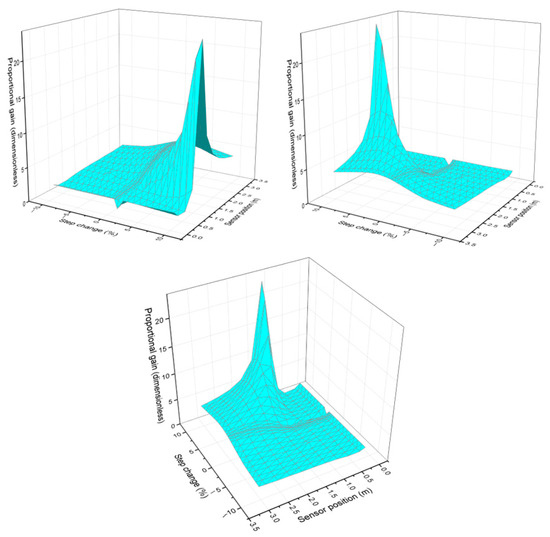
Figure 2.
Behavior of proportional gain as the step change and sensor position vary, seen from different perspectives.
For the final part of the reactor at this stage, most of the reactants have already been consumed, and the reaction is stopping. The amount of heat released is lower because less of the reaction is occurring. As a result, the system becomes more stable again, and temperature fluctuations are smaller; such a high proportional gain is not required because there is less to correct.
From the hot spot up to 2 m, the reaction is at its peak, meaning the reaction rate is maximum. Heat release is more intense, which can cause large temperature fluctuations. Because of this, the system becomes more unstable, as small changes can generate considerable temperature deviations. To mitigate these changes quickly, a higher proportional gain is needed. This means the controller must respond more quickly and more strongly to any temperature variation, preventing the system from spiraling out of control.
It was also observed that parameters such as gain change depending on the step size. For smaller steps (0.1 and 3%), the proportional gain is lower, and when larger steps are applied, such as 10%, the graph tends to distort and concentrate larger gain values. The deformation observed in the graph for large jumps can be interpreted as an indication that the system does not respond uniformly across the entire operating region. For small jumps, the graph shows a more uniform surface because the system maintains more predictable and stable behavior. For large step changes, the surface becomes more irregular and deformed, indicating that the system is in a region where the gain changes more drastically.
The response of the integral gain behavior as the step size and temperature sensor change (see Figure 3) is then analyzed. It is observed that the 3D graph exhibits greater deformation when large step sizes are implemented. As the step size increases, the variability in the PI gain intensifies, reflected in greater surface deformation on the graph. This suggests that characterizing the process with larger steps introduces more pronounced dynamic effects.
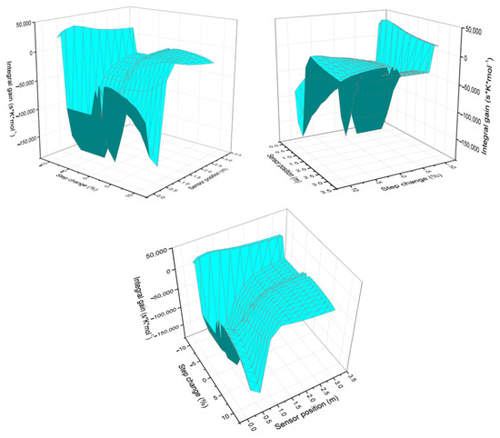
Figure 3.
Integral gain behavior as the step change and sensor position vary, viewed from different perspectives.
Regarding the influence of sensor position, the integral gain decreases in the region close to the hot spot (as reflected by the more negative values in the table and graph). Once the hot spot effect diminishes, the integral gain rises again, producing a canyon-like profile in the graph. This behavior highlights the strong dependence of the controller’s response on the sensor location.
Regarding the effects of sensor position, in the region near the hot spot, the integral gain tends to decrease (more negative values are observed in the table and graph). Subsequently, as the hot spot effect dissipates, the integral gain increases again, creating a canyon-like pattern on the graph. This indicates that the sensor location significantly influences the controller’s response.
The graph in Figure 3 shows that the effects of the hot spot are more noticeable when larger step sizes are applied. This suggests that the thermal impact on PI gain is amplified with larger changes in jacket temperature, which could be related to greater nonlinearity in the system dynamics.
Finally, Figure 4 analyzes the integral time response according to the variability of the sensor position and the chosen step size. It can be observed that the integral time decreases with increasing step size, indicating a general trend in which higher step sizes correspond to lower integral times. This may be because a larger input step results in a faster system response, reducing the need for lengthy integration.
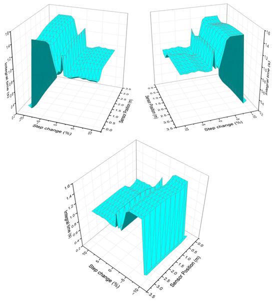
Figure 4.
Integral time behavior as the step change and sensor position vary from different perspectives.
The integral term in a PI controller accumulates the error over time and generates a corrective action based on the sum of past errors. If the error persists for a long time, the integral action continues to accumulate, resulting in a slower system response and a longer integral time. When the step size is small, the system response is slower, meaning the controller needs to accumulate more error over time before reaching the desired value. If the step size is large, the system’s response is faster, and less integral action is required to correct the error, which reduces the integral time. A larger deviation generates a stronger and faster response because the controller responds based on the error. If the error is larger, the controller generates a more intensive control action.
For small step changes, the integral time values are larger. On the other hand, it can be observed that when the step change size is smaller, the integral time is longer in several regions of the reactor. This may be because a small change in the input generates a slower system response, which prolongs the correction of the accumulated error.
The presence of the hot spot near 0.64 m is also a factor evident in the graph, since a band of low integral time values is observed in a region near 0.64 m. This suggests that the hot spot effect is influencing the dynamics of the control system, reducing the need for integral action in that area. This behavior may be related to greater sensitivity to heat transfer and chemical reaction in that part of the reactor.
3.2. Control System Evaluation
Twenty control strategies were designed using step changes in the jacket temperature ranging from −10% to +10% (−10, −9, …, −1, +1, …, +9, +10%). Each control was tested at four different sensor locations along the reactor length: near the inlet (5%), at the hot spot (20%), at 60%, and near the outlet (95%). Controls are evaluated with three types of disturbance sequences implemented:
Sequence 1: 10% benzene composition at 50 s;
Sequence 2: 10% feed temperature at 50 s;
Sequence 3: 10% benzene composition at 50 s and −10% of the feed temperature at 100 s.
To determine which position and step size provide the best control performance, the Absolute Error Integral is analyzed, as well as the selectivity and efficiency values obtained. Table A1, in Appendix A, presents the complete dataset, showing the reactor temperature (TR), jacket temperature (Tc), yield, selectivity, and Integral Absolute Error (IAE) values obtained after applying the corresponding feed disturbances and the control compensates them.
The results presented in Table A2 indicate that when the evaluation was carried out by applying a disturbance to the feed composition, for 17 of the 20 designed controllers, the best performance was obtained when the temperature sensor was placed at 95% of the reactor length.
When a 10% perturbation was applied to the feed temperature (see Table A2 in Appendix A), the location of the optimal sensor depended on the type of step used for controller design. Controllers designed with positive steps (+1% to +10%) achieved superior performance when the sensor was positioned at 60% of the reactor length. In contrast, controllers designed with negative steps (−1% to −10%) performed best with the sensor placed at 95% of the reactor length.
Finally, under combined disturbances (+10% in composition and +10% in feed temperature), 17 of the 20 controllers again showed the best performance when the sensor was located at 95% of the reactor length, as reported in Table A3. Overall, these results indicate that the most favorable control performance is consistently achieved when the temperature sensor is placed beyond the midpoint of the reactor, approaching the outlet, as confirmed by the Integral of Absolute Error (IAE) metric.
On the other hand, the reactor secondary controller with the lowest performance according to the IAE values is at the beginning of the reactor, at 5% of its length, and in some cases at the hot spot (20%). Near the reactor inlet, the reaction rate is high due to the high concentration of reactants introduced into the reactor. This can generate temperature increases, since the reaction rate and reactor temperature are directly related. The higher the reaction rate, the greater the heat release and the greater the sensitivity to external disturbances, which makes it difficult to control temperature and concentration.
In the intermediate zone of the reactor, concentrations have begun to decrease due to the consumption of reactants, so the reaction rate is moderate, reducing temperature fluctuations in the reactor. The zone after the hot spot exhibits smoother behavior because the reactant concentration there decreases, heat generation practically declines, and the disturbances that entered the system have already been mitigated throughout the reactor, significantly reducing the process sensitivity.
This same behavior has been reported by Van den Berg et al., (2000) [12], who developed robust selection criteria for the optimal location of concentration or temperature sensors and found that the optimal temperature sensor position for this same process is after the hot spot. Ramirez-Castelan et al., (2016) [17] performed a fractal analysis that allowed them to find the best temperature sensor position for a cascade control system in a tubular reactor, corroborating the results obtained in this research. Similarly, Urrea et al., (2008) [18] observed that the best place to position the sensor is after the hot spot, concluding that temperature measurements at the midpoint between the hot spot and the reactor outlet provide sensitive information to mitigate the adverse effects of the inlet conditions.
From Appendix A, mentioned above, the information for the best-performing control and the one with the least favorable performance was extracted. Table 1 shows the reactor temperature (TR), jacket temperature (Tc), efficiency, selectivity, and Integral Absolute Error (IAE) values for each of the three applied perturbation sequences. This selective representation aims to provide a concise and direct comparison between the extremes of our analysis: the control designed with a −9% step (which demonstrated the most favorable performance and is highlighted in blue) and the control designed with a 10% step (which showed the least favorable performance and is highlighted in gray). The results presented in this table serve to clearly and convincingly illustrate how the choice of step directly influences the operational stability and efficiency of the process, thus validating the main conclusions of this study. Some results from the table will be presented in the graphs below. The background color of the cells indicates control performance according to the Integral of Absolute Error (IAE): gray cells represent configurations with lower control performance, while blue cells correspond to configurations with higher control performance for each disturbance sequence applied.

Table 1.
Control system evaluation.
Comparing the transient response behavior of the maleic anhydride composition (product of interest), reactor temperature, jacket temperature, selectivity, and efficiency, the control designed with a 10% step exhibits a longer settling time compared to the performance of a tuned control system with a −9% step change.
Figure 5 shows the composition response when a 10% benzene feed disturbance occurs at 50 s for the two designed control systems.
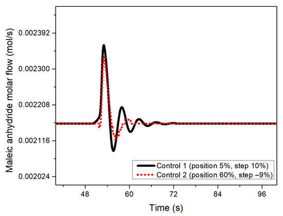
Figure 5.
Maleic anhydride flow behavior when a 10% disturbance at 50 s in the benzene feed was implemented for both designed controllers at 50 s.
Figure 6 shows the behavior of the jacket temperature and the reactor temperature when applying a 10% benzene feed disturbance.
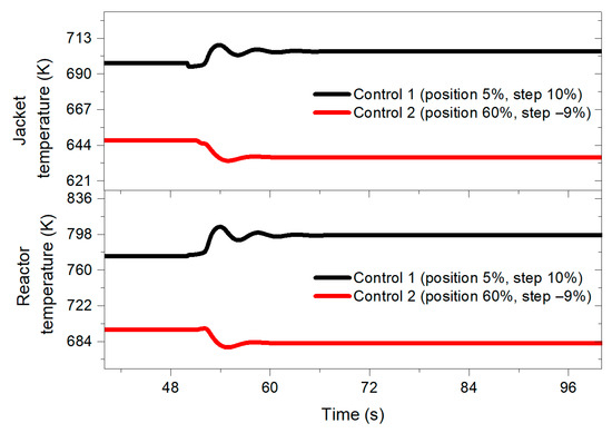
Figure 6.
Reactor and jacket temperature behavior when implementing a 10% perturbation in the benzene feed for both designed controllers at 50 s.
In both graphs (Figure 5 and Figure 6), it is possible to observe how the transient response of the control designed with the negative step is more mitigated by inducing the disturbance, presenting less pronounced oscillations. Similarly, the control structure designed with the 10% step shows a longer settling time compared to the performance of a control system tuned with a −9% step.
At the same time, it was noted that the selectivity values obtained increased (see Figure 7) with the control system designed with the aforementioned negative step, reaching percentages between 38 and 50% compared to controllers designed with the other step sizes (10% to −8%), which present values of 24 and 35%. On the other hand, the yield remained at the same values regardless of the step size chosen.
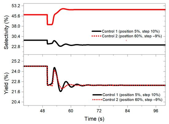
Figure 7.
Selectivity and yield behavior when implementing a 10% disturbance in the benzene feed for both controllers designed at 50 s.
Comparative analysis of the control system performance, based on the graphs and parameters in Table 1, revealed that the most effective tuning was performed with a −9% step in jacket temperature, significantly outperforming controls designed with a 10% step. This can be justified based on previous studies on the ideal operating conditions for the oxidation reaction of benzene to maleic anhydride.
These results are further supported by the study of Uraz and Atalay (2007) [19] showed that the oxidation of benzene, performed in a fluidized bed reactor using six different types of catalysts, was most effective in a temperature range of 325 to 400 °C (598.15 to 673.15 K). On the other hand, Phung Cuach et al., (1978) [20] noticed that benzene conversion increased with temperatures ranging from 280 °C to 430 °C (553.15 to 703.15 K), attributing it to the homogeneous thermal decomposition and oxidation of maleic anhydride at high temperatures. They mention that maleic anhydride selectivity increases with temperatures above 380 °C (653.15), while Dmuchovsky et al., (1965) [21] showed that using vanadia molybdenum increases selectivity up to 65% if the process is carried out at 377 °C (650.15 K). Uraz and Atalay (2012) [22] again studied the oxidation of benzene to maleic anhydride but this time comparing the performance in two types of reactor (fluidized bed reactor and a fixed bed reactor), using vanadium pentoxide as catalyst, considering the operating conditions of a temperature range between 300 and 400 °C.
Therefore, the literature supports that the oxidation reaction of benzene to maleic anhydride should be carried out in a range between 280 and 430 ° C (553.15 to 703.15 K) as previously mentioned, in the simulation carried out when a step change of −9% and −10% is used, a control system with a better performance is designed, in which the reactor temperature is maintained between a range of 375.074 to 412.62 ° C (648.224 to 685.77 K), on the other hand when a control is designed using step changes of 10% to −8% the reactor temperature is maintained at 465.35 ° C and 660.31 ° C (933.46 to 738.50 K), which exceeds the temperature ranges reported in the literature for the development of the reaction and, therefore, the selectivity of the process decreases drastically, adding to this that the process performance is lower compared to controls designed with a jump of −9 and −10%.
This may be due to the fact that, under the initial conditions, the process temperature (Tc = 697°K, equivalent to 423.85 °C, and the reactor temperature of 709°K, equivalent to 435.85 °C) is within the maximum limit suitable for the process to proceed, according to the literature. The exothermic nature of the reaction within the reactor, combined with a step change in the jacket temperature, can cause an increase in the internal temperature. If this temperature increase brings the system to the optimal operating range, secondary reactions are activated that decrease selectivity toward the desired product, maleic anhydride. The temperature increase has a direct effect on the catalyst’s efficiency, as excessive temperatures can cause its degradation or sintering, thus reducing its activity and leading to poor process performance. This confirms the importance of properly tuning a control system that maintains the temperature within safe limits.
Returning to the subject of the catalytic part, in this benzene oxidation process, vanadium pentoxide is used. In the work of Bielański et al., (1988) [23], it is mentioned that benzene oxidation is carried out in a temperature range of 300 to 400 ° C, observing that the stability of the catalyst, particularly of certain oxides such as V2O4 and V6O13, is greater in this temperature range, since they are the most resistant to chemical transformations during the reaction. They mention that these oxides showed the greatest stability at catalytic conditions at 350 ° C, evidencing that temperatures close to this parameter are optimal to continue working properly without the catalysts becoming less active.
Therefore, to operate the catalyst without compromising its effectiveness and avoiding its deactivation, it is located approximately at 350 ° C within the range of 300 to 400 ° C, as reported by the authors. This value appears to be the most appropriate to balance the activity and stability of the catalyst during the process. This finding is consistent with the research of Tufan & Akgerman (1981) [24], who performed reactions in a range of 344 to 393 °C and did not observe deactivation, since the temperature was kept below 400 °C, very far from the melting point of V2O5 (around 700 °C), again supporting that the appropriate temperature for the development of the reaction and taking care of the catalytic action is in ranges of 300 to 400 °C, which is achieved by tuning the control with jumps of −9%.
In order to describe the topography of 3D graphs regarding the behavior of control parameters, a fractality analysis is performed, verifying whether there is a relationship between the fractality index and the performance of the control system.
Fractal geometry is a way of describing the “texture” of a surface. There are four topological dimensions in traditional Euclidean geometry: 0-D for points, 1-D for straight lines, 2-D for planes, and 3-D for volumetric objects such as cubes and spheres. A “fractal” object has an intermediate dimensionality, such as 1.6 or 2.4. Generally, the higher the fractal dimension, the rougher the texture (Schowengerdt R. A. 2007) [25]. Fractal geometry provides a mathematical description of complex shapes not easily described by Euclidean geometry. It is consistent with the concept of spatial dimension, but is not limited to an integer. For example, a larger fractal dimension represents a more complex object or one that occupies the entire space (Yaffe, M. J., & Boyd, N. F. 2009) [26].
To perform the fractal analysis, each graph was analyzed individually by dividing it into four zones. The objective was to ensure an equitable distribution of the amount of data analyzed in each zone, in addition to having a large data population, since it was observed that a smaller data population can lead to ambiguous fractality indices.
The zones were considered as follows:
Zone 1: jump from 10% to 5%
Zone 2: jump from 5% to 0%
Zone 3: jump from 0% to −5%
Zone 4: jump from −5% to −10%
Figure 8 illustrates the divisions made to the graphs according to the aforementioned zones.
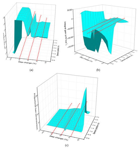
Figure 8.
Division of the 3D graphs of the control parameters into four zones. (a) Proportional gain graph, (b) the proportional–integral gain, and (c) integral time.
Once the control systems were evaluated and it was recognized that zone 4 provided the best performance (step increments of −5 to −10%, since the control systems designed with step increments of −9 and −10% performed better), the fractality index calculated for each zone was compared. The results are shown in Table 2.
Table 2.
Fractality index by zone.
The results in the table above show that the integral time graph presents the highest overall fractality index compared to the other two control parameters analyzed. This indicates that integral time is the parameter with the greatest changes in topography according to the variability of the step change and the sensor position.
On the other hand, the areas with positive step changes present a lower fractality index, especially for controls designed with steps of 10% to 5%; this fact is consistent with all three control parameters. Conversely, when negative steps are analyzed, the graph becomes more fractal, increasing the index value.
The fractality index indicates that the least fractal areas are those with positive steps (10% to 5%). Meanwhile, the control system performs better with negative steps (−9% and −10% located in zone 4). Therefore, there is an indirect relationship between fractality and control performance. The greater the fractality (a less predictable and more fluctuating topography), the better the control performance, and the lower the fractality (more predictable behavior), the worse the control system performance.
A higher fractality indicates a more complex topography, in which small changes can introduce less predictable behavior. A lower fractality indicates that the control parameters are more predictable and follow a more linear behavior, making it less difficult to find the parameter in the graph that falls within this zone of low fractality.
In contrast, control efficiency analysis (the evaluation of the control system after introducing disturbances) provides information on the control’s performance in handling disturbances. The control designed with negative steps, specifically −9% and −10%, performed better than the one designed with positive steps, as mentioned above. This is because with this step size, the process temperature is brought to the appropriate ranges within which the disturbance should occur, while the other steps tested lead to the reaction at unsuitable temperature limits.
The rough or fractal topography of control parameters should not be interpreted as an indication of instability, but rather as a manifestation of successful system adaptation to complex dynamics. The areas of the 3D graphs of control parameter behavior that exhibit the most irregular topography (highest fractality) are those that most effectively adjust to the nonlinear behavior of the process. This is because, rather than following a fixed pattern, the controller responds aggressively and variably to successfully address the complexity of the system, maintaining temperature and composition within optimal ranges.
The fractal analysis proposed in this study is not intended to replace conventional tuning methods, but rather to offer a complementary tool for characterizing the dynamic complexity and adaptability of the controller to the nonlinear nature of the process. The results obtained identify a correlation between a higher fractality index and better control performance, suggesting that fractal analysis could be used as an auxiliary criterion to guide the tuning of new systems exhibiting similar dynamic behaviors. However, we recognize that this potential predictive capability depends on certain assumptions, such as the structural similarity of the system and the type of step applied.
In summary, the superior performance of controllers designed with negative step sizes is attributed to their ability to adjust their parameters in a highly adaptive manner. This adaptability is crucial for countering process complexities in a demanding operating region. The fractal topography is, therefore, the visual representation of this adaptive capacity, demonstrating that successful control in a complex system often requires an equally complex and variable response. The strategy can be applied to a real reactor, as the proposed model was designed to reproduce the dynamic behavior of an industrial tubular reactor. While these findings highlight the potential applicability of the strategy to real industrial reactors since the proposed model reproduces the dynamic behavior of a tubular reactor, practical implementation involves certain limitations to be considered. In particular, industrial control systems typically perform measurements at discrete intervals (e.g., every 5 s) rather than continuously, creating brief gaps during which small variations in process variables may occur. Moreover, the resolution and sensitivity of industrial sensors may not be sufficient to detect minimal changes in temperature or composition, potentially reducing the controller’s responsiveness to subtle disturbances. Additional delays associated with the actuation of control elements, such as valves, can also affect the overall response time and accuracy of the system under real operating conditions.
4. Conclusions
This study demonstrated that the selection of the step size during controller design has a direct and decisive influence on the thermal stability and selectivity of the benzene oxidation process to maleic anhydride. The improved performance observed at the −9% step is primarily due to the genuine dynamics of the process, derived from the highly exothermic and multi-reactional nature of the benzene to maleic anhydride oxidation system. In this type of process, small temperature variations cause significant changes in reaction rates, which shift the equilibrium between desired and undesired reactions.
The shift in the operating point generated by the −9% step places the reactor within a temperature range (approximately 375 °C to 412 °C) where the primary reaction is more selective and thermally stable. In this range, heat generation decreases and secondary reactions are reduced, resulting in more favorable dynamics for cascade control: the inner temperature loop becomes faster, while the outer composition loop maintains a slower and more stable response. Therefore, the improved performance in this scenario reflects a real change in the system dynamics, not an artificial effect of the tuning method.
This finding highlights that a properly tuned step size not only prevents overheating but also significantly enhances process selectivity and operational safety.
Conversely, step changes between +10% and −8% led to reactor temperatures exceeding the safe operating range, resulting in catalyst deactivation and undesired by-product formation. These results emphasize that inappropriate controller tuning can critically compromise process efficiency. Regarding sensor position, the most favorable performance was obtained when the temperature sensor was located beyond the hot-spot zone (at 60% and 95% of reactor length), providing more representative temperature feedback and consistent control action.
Building upon these findings, sensor performance could be further improved by integrating advanced simulation tools and artificial intelligence techniques that allow their dynamics to be modeled and measurement errors to be compensated for in real time. This makes it possible to correct the limitations of the mathematical model, which sometimes cannot fully represent the complexity of the real process. The use of neural networks can also help estimate variables that are not directly measurable and predict them in real time, such as catalytic temperature. These strategies represent a promising avenue for future research, aimed at developing virtual and intelligent sensors capable of improving the stability and efficiency of nonlinear chemical processes.
Furthermore, the fractal analysis of the control surfaces further revealed an inverse relationship between fractality and control degradation: regions with higher fractal dimension—reflecting more complex and nonlinear dynamic behavior—corresponded to superior control performance, while low-fractal regions (particularly for positive step changes of +10% to +5%) exhibited poorer regulation. This confirms that fractal metrics can serve as a diagnostic and comparative tool for evaluating control performance in nonlinear systems.
In summary, this work provides practical design guidelines for cascade control systems applied to highly exothermic multi-reaction processes, demonstrating how controller tuning, step magnitude, and sensor placement influence process stability and selectivity. The findings have direct implications for the design and optimization of industrial reactors involving multiple exothermic reactions, particularly for improving control performance in processes such as the oxidation of aromatic hydrocarbons, polymerization, and catalytic oxidation in packed-bed and tubular configurations. By enhancing thermal stability and selectivity, the proposed approach supports safer and more energy-efficient operation, reducing the risk of runaway reactions and increasing product yield. Moreover, improved selectivity promotes a more effective conversion of reactants into the desired product, ensuring optimal utilization of raw materials, lower energy consumption, and a reduced environmental footprint. Overall, the proposed methodology offers a practical and scalable advantage for industrial applications involving strongly exothermic reaction systems.
Author Contributions
Conceptualization, M.M.J. and I.G.R.; Methodology, G.R.U.G.; Software, M.M.J. and I.G.R.; Validation, G.R.U.G.; Formal analysis, M.M.J. and I.G.R.; Investigation, M.M.J. and I.G.R.; Data curation, M.M.J. and I.G.R.; Writing—Original draft preparation, M.M.J.; Writing—Review and editing, G.L.S., C.S.R. and G.R.U.G.; Visualization, M.M.J.; Supervision, G.L.S., C.S.R. and G.R.U.G.; Project administration, G.R.U.G. All authors have read and agreed to the published version of the manuscript.
Funding
This research received no external funding.
Data Availability Statement
The original contributions of this study are included in the article. Further inquiries can be directed to the corresponding author.
Acknowledgments
The authors gratefully acknowledge the Tecnológico Nacional de México/Instituto Tecnológico de Orizaba for the institutional support provided during the development of this research. The authors also thank the reviewers for their valuable comments and constructive feedback, which greatly improved the quality of this work.
Conflicts of Interest
The authors declare no conflicts of interest. The research was conducted without any commercial or financial relationships that could be construed as a potential conflict of interest.
Abbreviations
The following abbreviations are used in this manuscript:
| Ai | Pre-exponential factor of the i-th simultaneous reaction |
| cs | Coefficient relating the molar flow to the heat capacity of the solid phase |
| Ei | Activation energy of the i-th simultaneous reaction |
| FMA | Molar flow of maleic anhydride |
| FB | Molar flow of benzene |
| IAE | Integral Absolute Error |
| ki | Reaction rate of the i-th simultaneous reaction |
| K | Gain |
| FOPDTM | First-Order Plus Dead Time Model |
| P | Proportional |
| PI | Proportional–Integral |
| R | Universal gas constant |
| t | Time |
| TC | Jacket temperature |
| TS | Solid phase temperature |
| TF | Fluid temperature |
| Us-f | Liquid film heat transfer coefficient for the jacket |
| Uf-c | Liquid film heat transfer coefficient for the jacket |
| z | Reactor length |
| ∆m | Step change magnitude |
| ∆Hi | Heat of the i-th reaction, i = 1, 2, 3 |
| θ | Time delay |
| τ | Integral time constant |
Appendix A
Table A1.
Control system response to a 10% disturbance in feed composition.
Table A1.
Control system response to a 10% disturbance in feed composition.
| Zone | Step | Parameter | 3.04 m (95%) | 1.92 m (60%) | 0.64 m (20%) | 0.16 m (5%) |
|---|---|---|---|---|---|---|
| Zone 1 | 10% | TR (K) | 738.50673 | 773.15722 | 933.46012 | 796.95867 |
| Tc (K) | 704.51586 | 704.51586 | 704.51586 | 704.51586 | ||
| Yield (%) | 22.37844 | 22.37844 | 22.37844 | 22.37844 | ||
| Selectivity (%) | 24.09332 | 24.09332 | 24.09332 | 24.09332 | ||
| IAE | 0.04689 | 0.04758 | 0.04999 | 0.05004 | ||
| 9% | TR (K) | 738.506731 | 773.157216 | 933.460125 | 796.958668 | |
| Tc (K) | 704.515859 | 704.515859 | 704.515859 | 704.515859 | ||
| Yield (%) | 22.378439 | 22.378439 | 22.378439 | 22.378439 | ||
| Selectivity (%) | 24.093324 | 24.093324 | 24.093324 | 24.093324 | ||
| IAE | 0.046667 | 0.047497 | 0.049225 | 0.048951 | ||
| 8% | TR (K) | 738.506731 | 773.157216 | 933.460125 | 796.958668 | |
| Tc (K) | 704.515859 | 704.515859 | 704.515859 | 704.515859 | ||
| Yield (%) | 22.378439 | 22.378439 | 22.378439 | 22.378439 | ||
| Selectivity (%) | 24.093324 | 24.093324 | 24.093324 | 24.093324 | ||
| IAE | 0.046527 | 0.047567 | 0.048579 | 0.048125 | ||
| 7% | TR (K) | 738.506731 | 773.157216 | 933.460125 | 796.958668 | |
| Tc (K) | 704.515859 | 704.515859 | 704.515859 | 704.515859 | ||
| Yield (%) | 22.378439 | 22.378439 | 22.378439 | 22.378439 | ||
| Selectivity (%) | 24.093324 | 24.093324 | 24.093324 | 24.093324 | ||
| IAE | 0.046438 | 0.047652 | 0.048250 | 0.047706 | ||
| 6% | TR (K) | 738.506731 | 773.157216 | 933.460125 | 796.958668 | |
| Tc (K) | 704.515859 | 704.515859 | 704.515859 | 704.515859 | ||
| Yield (%) | 22.378439 | 22.378439 | 22.378439 | 22.378439 | ||
| Selectivity (%) | 24.093324 | 24.093324 | 24.093324 | 24.093324 | ||
| IAE | 0.046411 | 0.047761 | 0.047920 | 0.047327 | ||
| Zone 2 | 5% | TR (K) | 738.506731 | 773.157216 | 933.460125 | 796.958668 |
| Tc (K) | 704.515859 | 704.515859 | 704.515859 | 704.515859 | ||
| Yield (%) | 22.378439 | 22.378439 | 22.378439 | 22.378439 | ||
| Selectivity (%) | 24.093324 | 24.093324 | 24.093324 | 24.093324 | ||
| IAE | 0.046383 | 0.047745 | 0.047722 | 0.047107 | ||
| 4% | TR (K) | 738.506731 | 773.157216 | 933.460125 | 796.958668 | |
| Tc (K) | 704.515859 | 704.515859 | 704.515859 | 704.515859 | ||
| Yield (%) | 22.378439 | 22.378439 | 22.378439 | 22.378439 | ||
| Selectivity (%) | 24.093324 | 24.093324 | 24.093324 | 24.093324 | ||
| IAE | 0.046409 | 0.047676 | 0.047535 | 0.046918 | ||
| 3% | TR (K) | 738.506731 | 773.157216 | 933.460125 | 796.958668 | |
| Tc (K) | 704.515859 | 704.515859 | 704.515859 | 704.515859 | ||
| Yield (%) | 22.378439 | 22.378439 | 22.378439 | 22.378439 | ||
| Selectivity (%) | 24.093324 | 24.093324 | 24.093324 | 24.093324 | ||
| IAE | 0.046443 | 0.047533 | 0.047410 | 0.046799 | ||
| 2% | TR (K) | 738.506731 | 773.157216 | 933.460125 | 796.958668 | |
| Tc (K) | 704.515859 | 704.515859 | 704.515859 | 704.515859 | ||
| Yield (%) | 22.378439 | 22.378439 | 22.378439 | 22.378439 | ||
| Selectivity (%) | 24.093324 | 24.093324 | 24.093324 | 24.093324 | ||
| IAE | 0.046447 | 0.047363 | 0.047330 | 0.046730 | ||
| 1% | TR (K) | 738.506731 | 773.157216 | 933.460125 | 796.958668 | |
| Tc (K) | 704.515859 | 704.515859 | 704.515859 | 704.515859 | ||
| Yield (%) | 22.378439 | 22.378439 | 22.378439 | 22.378439 | ||
| Selectivity (%) | 24.093324 | 24.093324 | 24.093324 | 24.093324 | ||
| IAE | 0.046421 | 0.047226 | 0.047238 | 0.046219 | ||
| Zone 3 | −1% | TR (K) | 738.506731 | 773.157216 | 933.460125 | 796.958668 |
| Tc (K) | 704.515859 | 704.515859 | 704.515859 | 704.515859 | ||
| Yield (%) | 22.378439 | 22.378439 | 22.378439 | 22.378439 | ||
| Selectivity (%) | 24.093324 | 24.093324 | 24.093324 | 24.093324 | ||
| IAE | 0.046477 | 0.047720 | 0.047749 | 0. 047288 | ||
| −2% | TR (K) | 738.506731 | 773.157216 | 933.460125 | 796.958668 | |
| Tc (K) | 704.515859 | 704.515859 | 704.515859 | 704.515859 | ||
| Yield (%) | 22.378439 | 22.378439 | 22.378439 | 22.378439 | ||
| Selectivity (%) | 24.093324 | 24.093324 | 24.093324 | 24. 093324 | ||
| IAE | 0.046590 | 0.050018 | 0.049949 | 0.049854 | ||
| −3% | TR (K) | 738.506731 | 773.157216 | 933.460125 | 796.958668 | |
| Tc (K) | 704.515859 | 704.515859 | 704.515859 | 704.515859 | ||
| Yield (%) | 22.378439 | 22.378439 | 22.378439 | 22.378439 | ||
| Selectivity (%) | 24.093324 | 24.093324 | 24.093324 | 24.093324 | ||
| IAE | 0.046018 | 0.048373 | 0.049113 | 0.048980 | ||
| −4% | TR (K) | 738.506731 | 773.157216 | 933.460125 | 796.958668 | |
| Tc (K) | 704.515859 | 704.515859 | 704.515859 | 704.515859 | ||
| Yield (%) | 22.378439 | 22.378439 | 22.378439 | 22.378439 | ||
| Selectivity (%) | 24.093324 | 24.093324 | 24.093324 | 24.093324 | ||
| IAE | 0.045904 | 0.048060 | 0.049026 | 0.048871 | ||
| −5% | TR (K) | 738.506731 | 773.157216 | 933.460125 | 796.958668 | |
| Tc (K) | 704.515859 | 704.515859 | 704.515859 | 704.515859 | ||
| Yield (%) | 22.378439 | 22.378439 | 22.378439 | 22.378439 | ||
| Selectivity (%) | 24.093324 | 24.093324 | 24.093324 | 24.093324 | ||
| IAE | 0.045871 | 0.047967 | 0.049026 | 0.048865 | ||
| Zone 4 | −6% | TR (K) | 738.506731 | 773.157216 | 933.460125 | 796.958668 |
| Tc (K) | 704.515859 | 704.515859 | 704.515859 | 704.515859 | ||
| Yield (%) | 22.378439 | 22.378439 | 22.378439 | 22.378439 | ||
| Selectivity (%) | 24.093324 | 24.093324 | 24.093324 | 24.093324 | ||
| IAE | 0. 045848 | 0.047941 | 0.049010 | 0.048864 | ||
| −7% | TR (K) | 738.506731 | 773.157216 | 933.460125 | 796.958668 | |
| Tc (K) | 704.515859 | 704.515859 | 704.515859 | 704.515859 | ||
| Yield (%) | 22.378439 | 22.378439 | 22.378439 | 22.378439 | ||
| Selectivity (%) | 24.093324 | 24.093324 | 24.093324 | 24.093324 | ||
| IAE | 0.045833 | 0.047920 | 0.049003 | 0.048875 | ||
| −8% | TR (K) | 738.506731 | 773.157216 | 933.460125 | 796.958668 | |
| Tc (K) | 704.515859 | 704.515859 | 704.515859 | 704.515859 | ||
| Yield (%) | 22.378439 | 22.378439 | 22.378439 | 22.378439 | ||
| Selectivity (%) | 24.093324 | 24.093324 | 24.093324 | 24.093324 | ||
| IAE | 0.045815 | 0.047903 | 0.04898 | 0.048881 | ||
| −9% | TR (K) | 675.204051 | 682.115014 | 690.653198 | 648.224513 | |
| Tc (K) | 636.196168 | 636.196168 | 636.196168 | 636.595215 | ||
| Yield (%) | 22.378439 | 22.378439 | 22.378439 | 22.378439 | ||
| Selectivity (%) | 50.426878 | 50.426878 | 50.426878 | 50.692474 | ||
| IAE | 0.044199 | 0.044151 | 0.044283 | 0.044622 | ||
| −10% | TR (K) | 675.204051 | 682.115014 | 690.653198 | 668.830166 | |
| Tc (K) | 636.196168 | 636.196168 | 636.196168 | 636.196168 | ||
| Yield (%) | 22.378439 | 22.378439 | 22.378439 | 22.378439 | ||
| Selectivity (%) | 50.426878 | 50.426878 | 50.426878 | 50.426878 | ||
| IAE | 0.044761 | 0.044721 | 0.045071 | 0.045130 |
Table A2.
Control system response to a 10% disturbance in feed temperature.
Table A2.
Control system response to a 10% disturbance in feed temperature.
| Zone | Step | Parameter | 3.04 m (95%) | 1.92 m (60%) | 0.64 m (20%) | 0.16 m (5%) |
|---|---|---|---|---|---|---|
| Zone 1 | 10% | TR (K) | 731.209117 | 761.123611 | 865.91278 | 810.3801 |
| Tc (K) | 695.358144 | 695.358144 | 695.35814 | 695.35814 | ||
| Yield (%) | 24.616283 | 24.616283 | 24.61628 | 24.61628 | ||
| Selectivity (%) | 27.743812 | 27.743812 | 27.74381 | 27.74381 | ||
| IAE | 0.046085 | 0.045471 | 0.04922 | 0.04992 | ||
| 9% | TR (K) | 731.209117 | 761.123611 | 865.912781 | 810.380104 | |
| Tc (K) | 695.358144 | 695.358144 | 695.358144 | 695.358144 | ||
| Yield (%) | 24.616283 | 24.616283 | 24.616283 | 24.616283 | ||
| Selectivity (%) | 27.743812 | 27.743812 | 27.743812 | 27.743812 | ||
| IAE | 0.045799 | 0.045160 | 0.048421 | 0.048870 | ||
| 8% | TR (K) | 731.209117 | 761.123611 | 865.912781 | 810.380104 | |
| Tc (K) | 695.358144 | 695.358144 | 695.358144 | 695.358144 | ||
| Yield (%) | 24.616283 | 24.616283 | 24.616283 | 24.616283 | ||
| Selectivity (%) | 27.743812 | 27.743812 | 27.743812 | 27.743812 | ||
| IAE | 0.045574 | 0.044951 | 0.047723 | 0.048071 | ||
| 7% | TR (K) | 731.209117 | 761.123611 | 865.912781 | 810.380104 | |
| Tc (K) | 695.358144 | 695.358144 | 695.358144 | 695.358144 | ||
| Yield (%) | 24.616283 | 24.616283 | 24.616283 | 24.616283 | ||
| Selectivity (%) | 27.743812 | 27.743812 | 27.743812 | 27.743812 | ||
| IAE | 0.045420 | 0.044846 | 0.047355 | 0.047666 | ||
| 6% | TR (K) | 731.209117 | 761.123611 | 865.912781 | 810.380104 | |
| Tc (K) | 695.358144 | 695.358144 | 695.358144 | 695.358144 | ||
| Yield (%) | 24.616283 | 24.616283 | 24.616283 | 24.616283 | ||
| Selectivity (%) | 27.743812 | 27.743812 | 27.743812 | 27.743812 | ||
| IAE | 0.045306 | 0.044784 | 0.046966 | 0.047301 | ||
| Zone 2 | 5% | TR (K) | 731.209117 | 761.123611 | 865.912781 | 810.380104 |
| Tc (K) | 695.358144 | 695.358144 | 695.358144 | 695.358144 | ||
| Yield (%) | 24.616283 | 24.616283 | 24.616283 | 24.616283 | ||
| Selectivity (%) | 27.743812 | 27.743812 | 27.743812 | 27.743812 | ||
| IAE | 0.045213 | 0.044764 | 0.046724 | 0.047090 | ||
| 4% | TR (K) | 731.209117 | 761.123611 | 865.912781 | 810.380104 | |
| Tc (K) | 695.358144 | 695.358144 | 695.358144 | 695.358144 | ||
| Yield (%) | 24.616283 | 24.616283 | 24.616283 | 24.616283 | ||
| Selectivity (%) | 27.743812 | 27.743812 | 27.743812 | 27.743812 | ||
| IAE | 0.045163 | 0.044778 | 0.046476 | 0.046908 | ||
| 3% | TR (K) | 731.209117 | 761.123611 | 865.912781 | 810.380104 | |
| Tc (K) | 695.358144 | 695.358144 | 695.358144 | 695.358144 | ||
| Yield (%) | 24.616283 | 24.616283 | 24.616283 | 24.616283 | ||
| Selectivity (%) | 27.743812 | 27.743812 | 27.743812 | 27.743812 | ||
| IAE | 0.045143 | 0.044835 | 0.046296 | 0.046795 | ||
| 2% | TR (K) | 731.209117 | 761.123611 | 865.912781 | 810.380104 | |
| Tc (K) | 695.358144 | 695.358144 | 695.358144 | 695.358144 | ||
| Yield (%) | 24.616283 | 24.616283 | 24.616283 | 24.616283 | ||
| Selectivity (%) | 27.743812 | 27.743812 | 27.743812 | 27.743812 | ||
| IAE | 0.045132 | 0.044934 | 0.046176 | 0.046731 | ||
| 1% | TR (K) | 731.209117 | 761.123611 | 865.912781 | 810.380104 | |
| Tc (K) | 695.358144 | 695.358144 | 695.358144 | 695.358144 | ||
| Yield (%) | 24.616283 | 24.616283 | 24.616283 | 24.616283 | ||
| Selectivity (%) | 27.743812 | 27.743812 | 27.743812 | 27.743812 | ||
| IAE | 0.045148 | 0.045106 | 0.046072 | 0.045868 | ||
| Zone 3 | −1% | TR (K) | 731.209117 | 761.123611 | 865.912781 | 810.380104 |
| Tc (K) | 695.358144 | 695.358144 | 695.358144 | 695.358144 | ||
| Yield (%) | 24.616283 | 24.616283 | 24. 616283 | 24.616283 | ||
| Selectivity (%) | 27.743812 | 27.743812 | 27.743812 | 27.743812 | ||
| IAE | 0.045463 | 0.046151 | 0.046731 | 0.047264 | ||
| −2% | TR (K) | 731.209117 | 761.123611 | 865.912781 | 810.380104 | |
| Tc (K) | 695.358144 | 695.358144 | 695.358144 | 695.358144 | ||
| Yield (%) | 24.616283 | 24.616283 | 24.616283 | 24.616283 | ||
| Selectivity (%) | 27.743812 | 27.743812 | 27.743812 | 27.743812 | ||
| IAE | 0.045904 | 0.048750 | 0.049197 | 0.049762 | ||
| −3% | TR (K) | 731.209117 | 761.123611 | 865.912781 | 810.380104 | |
| Tc (K) | 695.358144 | 695.358144 | 695.358144 | 695.358144 | ||
| Yield (%) | 24.616283 | 24.616283 | 24.616283 | 24.616283 | ||
| Selectivity (%) | 27.743812 | 27.743812 | 27.743812 | 27.743812 | ||
| IAE | 0.045348 | 0.047385 | 0.048338 | 0.048932 | ||
| −4% | TR (K) | 731.209117 | 761.123611 | 865.912781 | 810.380104 | |
| Tc (K) | 695.358144 | 695.358144 | 695.358144 | 695.358144 | ||
| Yield (%) | 24.616283 | 24.616283 | 24.616283 | 24.616283 | ||
| Selectivity (%) | 27.743812 | 27.743812 | 27.743812 | 27.743812 | ||
| IAE | 0.045232 | 0.047109 | 0.048246 | 0.048829 | ||
| −5% | TR (K) | 731.209117 | 761.123611 | 865.912781 | 810.380104 | |
| Tc (K) | 695.358144 | 695.358144 | 695.358144 | 695.358144 | ||
| Yield (%) | 24.616283 | 24.616283 | 24.616283 | 24.616283 | ||
| Selectivity (%) | 27.743812 | 27.743812 | 27.743812 | 27.743812 | ||
| IAE | 0.045197 | 0.047027 | 0.048245 | 0.048822 | ||
| Zone 4 | −6% | TR (K) | 731.209117 | 761.123611 | 865.912781 | 810.380104 |
| Tc (K) | 695.358144 | 695.358144 | 695.358144 | 695.358144 | ||
| Yield (%) | 24.616283 | 24.616283 | 24.616283 | 24.616283 | ||
| Selectivity (%) | 27.743812 | 27.743812 | 27.743812 | 27.743812 | ||
| IAE | 0.045172 | 0.047004 | 0.048229 | 0.048820 | ||
| −7% | TR (K) | 731.209117 | 761.123611 | 865.912781 | 810.380104 | |
| Tc (K) | 695.358144 | 695.358144 | 695.358144 | 695.358144 | ||
| Yield (%) | 24.616283 | 24.616283 | 24.616283 | 24.616283 | ||
| Selectivity (%) | 27.743812 | 27.743812 | 27.743812 | 27.743812 | ||
| IAE | 0.045155 | 0.046985 | 0.048222 | 0.048833 | ||
| −8% | TR (K) | 731.209117 | 761.123611 | 865.912781 | 810.380104 | |
| Tc (K) | 695.358144 | 695.358144 | 695.358144 | 695.358144 | ||
| Yield (%) | 24.616283 | 24.616283 | 24.616283 | 24.616283 | ||
| Selectivity (%) | 27.743812 | 27.743812 | 27.743812 | 27.743812 | ||
| IAE | 0.045136 | 0.046970 | 0.048208 | 0.048839 | ||
| −9% | TR (K) | 685.777153 | 695.131626 | 708.726068 | 710.565877 | |
| Tc (K) | 646.698892 | 646.698892 | 646.698892 | 646.698892 | ||
| Yield (%) | 24.616283 | 24.616283 | 24.616283 | 24.616283 | ||
| Selectivity (%) | 46.191636 | 46.191636 | 46.191636 | 46.191636 | ||
| IAE | 0.043709 | 0.043781 | 0.043908 | 0.044211 | ||
| −10% | TR (K) | 685.777153 | 695.131626 | 708.726068 | 710.565877 | |
| Tc (K) | 646.698892 | 646.698892 | 646.698892 | 646.698892 | ||
| Yield (%) | 24.616283 | 24.616283 | 24.616283 | 24.616283 | ||
| Selectivity (%) | 46.191636 | 46.191636 | 46.191636 | 46.191636 | ||
| IAE | 0.044223 | 0.044306 | 0.044697 | 0.045049 |
Table A3.
Control system response to a 10% disturbance in benzene feed composition and −10% disturbance in feed temperature.
Table A3.
Control system response to a 10% disturbance in benzene feed composition and −10% disturbance in feed temperature.
| Zone | Step | Parameter | 3.04 m (95%) | 1.92 m (60%) | 0.64 m (20%) | 0.16 m (5%) |
|---|---|---|---|---|---|---|
| Zone 1 | 10% | TR (K) | 736.90046 | 769.99242 | 928.02369 | 836.19874 |
| Tc (K) | 703.1152 | 703.1152 | 703.1152 | 703.1152 | ||
| Yield (%) | 22.37844 | 22.37844 | 22.37844 | 22.37844 | ||
| Selectivity (%) | 24.15366 | 24.15366 | 24.15366 | 24.15366 | ||
| IAE | 0.04657 | 0.04641 | 0.04983 | 0.05181 | ||
| 9% | TR (K) | 739.695790 | 775.555659 | 937.242681 | 763.897356 | |
| Tc (K) | 705.571136 | 705.571136 | 705.571136 | 705.571136 | ||
| Yield (%) | 22.378439 | 22.378439 | 22.378439 | 22.378439 | ||
| Selectivity (%) | 24.047055 | 24.047055 | 24.047055 | 24.047055 | ||
| IAE | 0.046693 | 0.047702 | 0.049231 | 0.049816 | ||
| 8% | TR (K) | 739.695790 | 775.555659 | 937.242681 | 763.897356 | |
| Tc (K) | 705.571136 | 705.571136 | 705.571136 | 705.571136 | ||
| Yield (%) | 22.378439 | 22.378439 | 22.378439 | 22.378439 | ||
| Selectivity (%) | 24.047055 | 24.047055 | 24.047055 | 24.047055 | ||
| IAE | 0.046557 | 0.047812 | 0.048586 | 0.049073 | ||
| 7% | TR (K) | 739.695790 | 775.555659 | 937.242681 | 763.897356 | |
| Tc (K) | 705.571136 | 705.571136 | 705.571136 | 705.571136 | ||
| Yield (%) | 22.378439 | 22.378439 | 22.378439 | 22.378439 | ||
| Selectivity (%) | 24.047055 | 24.047055 | 24.047055 | 24.047055 | ||
| IAE | 0.046471 | 0.047917 | 0.048257 | 0.048714 | ||
| 6% | TR (K) | 739.695790 | 775.55565 | 937.242681 | 763.897356 | |
| Tc (K) | 705.571136 | 705.571136 | 705.571136 | 705.571136 | ||
| Yield (%) | 22.378439 | 22.378439 | 22.378439 | 22.378439 | ||
| Selectivity (%) | 24.047055 | 24.047055 | 24.047055 | 24.047055 | ||
| IAE | 0.046449 | 0.048045 | 0.047927 | 0.048424 | ||
| Zone 2 | 5% | TR (K) | 739.695790 | 775.555659 | 937.242681 | 763.897356 |
| Tc (K) | 705.571136 | 705.571136 | 705.571136 | 705.571136 | ||
| Yield (%) | 22.378439 | 22.378439 | 22.378439 | 22.378439 | ||
| Selectivity (%) | 24.047055 | 24.047055 | 24.047055 | 24.047055 | ||
| IAE | 0.046424 | 0.048027 | 0.047729 | 0.048264 | ||
| 4% | TR (K) | 739.695790 | 775.555659 | 937.242681 | 763.897356 | |
| Tc (K) | 705.571136 | 705.571136 | 705.571136 | 705.571136 | ||
| Yield (%) | 22.378439 | 22.378439 | 22.378439 | 22.378439 | ||
| Selectivity (%) | 24.047055 | 24.047055 | 24.047055 | 24.047055 | ||
| IAE | 0.046454 | 0.047946 | 0.047542 | 0.048158 | ||
| 3% | TR (K) | 739.695790 | 775.555659 | 937.242681 | 763.897356 | |
| Tc (K) | 705.571136 | 705.571136 | 705.571136 | 705.571136 | ||
| Yield (%) | 22.378439 | 22.378439 | 22.378439 | 22.378439 | ||
| Selectivity (%) | 24.047055 | 24.047055 | 24.047055 | 24.047055 | ||
| IAE | 0.046491 | 0.047777 | 0.047418 | 0.048109 | ||
| 2% | TR (K) | 739.695790 | 775.555659 | 937.242681 | 763.897356 | |
| Tc (K) | 705.571136 | 705.571136 | 705.571136 | 705.571136 | ||
| Yield (%) | 22.378439 | 22.378439 | 22.378439 | 22.378439 | ||
| Selectivity (%) | 24.047055 | 24.047055 | 24.047055 | 24.047055 | ||
| IAE | 0.046495 | 0.047575 | 0.047338 | 0.048084 | ||
| 1% | TR (K) | 739.695790 | 775.555659 | 937.242681 | 763.897356 | |
| Tc (K) | 705.571136 | 705.571136 | 705.571136 | 705.571136 | ||
| Yield (%) | 22.378439 | 22.378439 | 22.378439 | 22.378439 | ||
| Selectivity (%) | 24.047055 | 24.047055 | 24.047055 | 24.047055 | ||
| IAE | 0.046467 | 0.047397 | 0.047245 | 0.047133 | ||
| Zone 3 | −1% | TR (K) | 739.695790 | 775.555659 | 937.242681 | 763.897356 |
| Tc (K) | 705.571136 | 705.571136 | 705.571136 | 705.571136 | ||
| Yield (%) | 22.378439 | 22.378439 | 22.378439 | 22.378439 | ||
| Selectivity (%) | 24.047055 | 24.047055 | 24.047055 | 24.047055 | ||
| IAE | 0.046511 | 0.047823 | 0.047755 | 0.048404 | ||
| −2% | TR (K) | 739.695790 | 775.555659 | 937.242681 | 763.897356 | |
| Tc (K) | 705.571136 | 705.571136 | 705.571136 | 705.571136 | ||
| Yield (%) | 22.378439 | 22.378439 | 22.378439 | 22.378439 | ||
| Selectivity (%) | 24.047055 | 24.047055 | 24.047055 | 24.047055 | ||
| IAE | 0.046609 | 0.050083 | 0.049954 | 0.050615 | ||
| −3% | TR (K) | 739.695790 | 775.555659 | 937.242681 | 763.897356 | |
| Tc (K) | 705.571136 | 705.571136 | 705.571136 | 705.571136 | ||
| Yield (%) | 22.378439 | 22.378439 | 22.378439 | 22.378439 | ||
| Selectivity (%) | 24.047055 | 24.047055 | 24.047055 | 24.047055 | ||
| IAE | 0.046038 | 0.048426 | 0.049118 | 0.049752 | ||
| −4% | TR (K) | 739.695790 | 775.555659 | 937.242681 | 763.897356 | |
| Tc (K) | 705.571136 | 705.571136 | 705.571136 | 705.571136 | ||
| Yield (%) | 22.378439 | 22.378439 | 22.378439 | 22.378439 | ||
| Selectivity (%) | 24.047055 | 24.047055 | 24.047055 | 24.047055 | ||
| IAE | 0.045924 | 0.048111 | 0.049032 | 0.049648 | ||
| −5% | TR (K) | 739.695790 | 775.555659 | 937.242681 | 763.897356 | |
| Tc (K) | 705.571136 | 705.571136 | 705.571136 | 705.571136 | ||
| Yield (%) | 22.378439 | 22.378439 | 22.378439 | 22.378439 | ||
| Selectivity (%) | 24.047055 | 24.047055 | 24.047055 | 24.047055 | ||
| IAE | 0.045891 | 0.048017 | 0.049031 | 0.049640 | ||
| Zone 4 | −6% | TR (K) | 739.695790 | 775.555659 | 937.242681 | 763.897356 |
| Tc (K) | 705.571136 | 705.571136 | 705.571136 | 705.571136 | ||
| Yield (%) | 22.378439 | 22.378439 | 22.378439 | 22.378439 | ||
| Selectivity (%) | 24.047055 | 24.047055 | 24.047055 | 24.047055 | ||
| IAE | 0.045868 | 0.047991 | 0.049016 | 0.049639 | ||
| −7% | TR (K) | 739.695790 | 775.555659 | 937.242681 | 763.897356 | |
| Tc (K) | 705.571136 | 705.571136 | 705.571136 | 705.571136 | ||
| Yield (%) | 22.378439 | 22.378439 | 22.378439 | 22.378439 | ||
| Selectivity (%) | 24.047055 | 24.047055 | 24.047055 | 24.047055 | ||
| IAE | 0.045853 | 0.047970 | 0.049008 | 0.049653 | ||
| −8% | TR (K) | 739.695790 | 775.555659 | 937.242681 | 763.897356 | |
| Tc (K) | 705.571136 | 705.571136 | 705.571136 | 705.571136 | ||
| Yield (%) | 22.378439 | 22.378439 | 22.378439 | 22.378439 | ||
| Selectivity (%) | 24.047055 | 24.047055 | 24.047055 | 24.047055 | ||
| IAE | 0.045835 | 0.047953 | 0.048994 | 0.049659 | ||
| −9% | TR (K) | 676.109678 | 683.196717 | 691.465401 | 648.224513 | |
| Tc (K) | 636.595215 | 636.595215 | 636.595215 | 636.595215 | ||
| Yield (%) | 22.378439 | 22.378439 | 22.378439 | 22.378439 | ||
| Selectivity (%) | 50.692474 | 50.692474 | 50.692474 | 50.692474 | ||
| IAE | 0.044200 | 0.044153 | 0.044283 | 0.044622 | ||
| −10% | TR (K) | 676.109678 | 683.196717 | 691.465401 | 648.224513 | |
| Tc (K) | 636.595215 | 636.595215 | 636.595215 | 636.595215 | ||
| Yield (%) | 22.378439 | 22.378439 | 22.378439 | 22.378439 | ||
| Selectivity (%) | 50.692474 | 50.692474 | 50.692474 | 50.692474 | ||
| IAE | 0.044763 | 0.044722 | 0.045071 | 0.045458 |
References
- Nise, N.S. Control Systems Engineering, 8th ed.; Wiley: Hoboken, NJ, USA, 2019; pp. 4–6. [Google Scholar]
- Burns, R. Advanced Control Engineering; Elsevier Science: Oxford, UK, 2001; pp. 1–3. [Google Scholar]
- Dorf, R.C.; Bishop, R.H. Modern Control Systems, 13th ed.; Pearson: Hoboken, NJ, USA, 2016. [Google Scholar]
- Cheng, Z.; Li, L.; Zhong, C.; Wang, J.; Bai, X.; Liu, J. Adaptive Nonlinear Active Disturbance Rejection Current Controller for Distributed Generation System Considering Uncertain Ripples. IEEE Trans. Power Electron. 2025, 40, 4984–4996. [Google Scholar] [CrossRef]
- Zhang, X.; Liu, Y.; Chen, X.; Li, Z.; Su, C.-Y. Adaptive Pseudoinverse Control for Constrained Hysteretic Nonlinear Systems and Its Application on Dielectric Elastomer Actuator. IEEE/ASME Trans. Mechatron. 2023, 28, 2142–2154. [Google Scholar] [CrossRef]
- Li, Y.; Jiang, Y.; Lu, J.; Tan, C. Improved Active Disturbance Rejection Control for Electro-Hydrostatic Actuators via Actor–Critic Reinforcement Learning. Eng. Appl. Artif. Intell. 2025, 158, 111485. [Google Scholar] [CrossRef]
- Trivedi, B.C.; Culbertson, B.M. Maleic Anhydride; Plenum Press: New York, NY, USA, 1982; pp. 1–40. [Google Scholar]
- McMullen, R.L. Maleic Anhydride Applications in Personal Care. In Handbook of Maleic Anhydride Based Materials; Musa, O., Ed.; Springer: Cham, Switzerland, 2016; pp. 441–507. [Google Scholar] [CrossRef]
- Hood, D.K.; Musa, O.M. Application of Maleic Anhydride in Coatings, Adhesives and Printing. In Handbook of Maleic Anhydride Based Materials; Musa, O., Ed.; Springer: Cham, Switzerland, 2016; pp. 509–575. [Google Scholar] [CrossRef]
- Cortes-Barreda, J.; Hernandez-Espinosa, J.; Urrea-García, G.R.; Luna-Solano, G.; Cantu-Lozano, D. Implementation of Software for the Determination of Modeling Error in a Tubular Reactor. In New Perspectives in Software Engineering. CIMPS 2020; Mejia, J., Muñoz, M., Rocha, Á., Quiñonez, Y., Eds.; Advances in Intelligent Systems and Computing; Springer: Cham, Switzerland, 2021; Volume 1297. [Google Scholar] [CrossRef]
- Urrea-García, G.R.; Reséndiz-Camacho, S.; Álvarez-Ramírez, J.; Luna-Solano, G. Variable Cascade Control Structure for Tubular Reactors. Chem. Eng. Technol. 2015, 38, 521–529. [Google Scholar] [CrossRef]
- Van den Berg, F.W.J.; Hoefsloot, H.C.J.; Boelens, H.F.M.; Smilde, A.K. Selection of optimal sensor position in a tubular reactor using robust degree of observability criteria. Chem. Eng. Sci. 2000, 55, 827–837. [Google Scholar] [CrossRef]
- Smith, C.A.; Corripio, A.B. Control Automático de Procesos, Teoría y Práctica, 2nd ed.; Limusa/Wiley: Mexico City, Mexico, 2014. [Google Scholar]
- Skogestad, S.; Grimholt, C. The SIMC Method for Smooth PID Controller Tuning. In PID Control in the Third Millennium; Vilanova, R., Visioli, A., Eds.; Springer: London, UK, 2012; pp. 147–174. [Google Scholar] [CrossRef]
- Hernández-Espinosa, J.; Urrea-García, G.R.; Luna-Solano, G. Estructura de Control Variable en Cascada para Compensar Variaciones en Parámetros en un Reactor Tubular. In Proceedings of the Congreso Nacional de Control Automático 2017, Monterrey, Nuevo León, México, 4–6 October 2017; Tecnológico Nacional de México, Instituto Tecnológico de Orizaba: Orizaba, Mexico, 2018. [Google Scholar]
- Wu, W.; Huang, M.-Y. Nonlinear Inferential Control for an Exothermic Packed-Bed Reactor: Geometric Approaches. Chem. Eng. Sci. 2003, 58, 2023–2034. [Google Scholar] [CrossRef]
- Ramirez-Castelan, C.E.; Moguel-Castañeda, J.; Puebla, H.; Hernandez-Martinez, E. A study of temperature sensor location based on fractal analysis for cascade control schemes in tubular reactors. Chem. Eng. Sci. 2016, 141, 195–204. [Google Scholar] [CrossRef][Green Version]
- Urrea, R.; Alvarez, J.; Alvarez-Ramirez, J. Linear PI Temperature-Concentration Cascade Control for Tubular Reactors. Chem. Eng. Commun. 2008, 195, 803–820. [Google Scholar] [CrossRef]
- Uraz, C.; Atalay, S. Oxidation of Benzene to Maleic Anhydride in a Fluidized Bed Reactor. Chem. Eng. Technol. 2007, 30, 1708–1715. [Google Scholar] [CrossRef]
- Phung Quach, T.Q.; Rouleau, D.; Chavarze, C.; Laguerze, C. Catalytic Oxidation of Benzene to Maleic Anhydride in a Continuous Stirred Tank Reactor. Can. J. Chem. Eng. 1978, 56, 72–78. [Google Scholar] [CrossRef]
- Dmuchovsky, B.; Freerks, M.C.; Pierron, E.D.; Munch, R.H.; Zienty, F.B. A study of the catalytic oxidation of benzene to maleic anhydride. J. Catal. 1965, 4, 291–300. [Google Scholar] [CrossRef]
- Uraz, C.; Atalay, S. Comparison between the performances of a fluidized-bed reactor and a fixed-bed reactor for the oxidation of benzene to maleic anhydride. Turk. J. Eng. Env. Sci. 2012, 36, 59–71. [Google Scholar] [CrossRef]
- Bielański, A.; Piwowarczyk, J.; Poźniczek, J. Catalytic Activity of Vanadium Oxides in the Oxidation of Benzene. J. Catal. 1988, 113, 334–340. [Google Scholar] [CrossRef]
- Tufan, G.; Akgerman, A. Kinetics of benzene oxidation over a vanadium oxide (V2O5) catalyst. Ind. Eng. Chem. Proc. Des. Dev. 1981, 20, 604–608. [Google Scholar] [CrossRef]
- Schowengerdt, R.A. Data Models. In Remote Sensing: Models and Methods for Image Processing, 3rd ed.; Schowengerdt, R.A., Ed.; Academic Press: Cambridge, MA, USA, 2007; pp. 127–182. [Google Scholar] [CrossRef]
- Yaffe, M.J.; Boyd, N.F. Quantitative Image Analysis for Estimation of Breast Cancer Risk. In Handbook of Medical Image Processing and Analysis, 2nd ed.; Bankman, I.N., Ed.; Academic Press: Cambridge, MA, USA, 2009; pp. 381–398. [Google Scholar] [CrossRef]


Disclaimer/Publisher’s Note: The statements, opinions and data contained in all publications are solely those of the individual author(s) and contributor(s) and not of MDPI and/or the editor(s). MDPI and/or the editor(s) disclaim responsibility for any injury to people or property resulting from any ideas, methods, instructions or products referred to in the content. |
© 2025 by the authors. Licensee MDPI, Basel, Switzerland. This article is an open access article distributed under the terms and conditions of the Creative Commons Attribution (CC BY) license (https://creativecommons.org/licenses/by/4.0/).