Attention-Enhanced Conditional Wasserstein GAN with Wavelet–ResNet for Fault Diagnosis Under Imbalanced Data

Abstract

Rolling bearings are critical components in mechanical systems, and their health directly affects operational reliability and safety. However, their exposure to harsh conditions makes accurate fault diagnosis essential. Conventional methods relying on expert knowledge and handcrafted features are inefficient, while deep learning still suffers from data imbalance, which limits generalization. To address this challenge, an Attention-Enhanced Conditional Wasserstein GAN (ACWGAN) is proposed, in which the attention mechanism is incorporated into both the generator and discriminator to capture global dependencies and enhance feature diversity. By combining attention guidance with the Wasserstein distance, the framework achieves more stable training, alleviates mode collapse, and generates high-fidelity fault samples to balance imbalanced datasets. Compared with existing GAN-based methods, this method, combined with wavelet-based ResNet, significantly improves the accuracy of diagnosis, achieving 100% accuracy in the generated dataset.

1. Introduction

With the continuous growth of modern industry, rotating machinery, including pumps, engines, and conveyor systems, has become widely employed in diverse applications [1]. Among their key components, rolling bearings are indispensable for reducing friction and ensuring smooth operation [2]. However, under extreme conditions such as high temperature, heavy load, and high speed, bearings are prone to wear and degradation. It is estimated that nearly $41\%$ of machinery failures are attributable to bearing faults [3], highlighting the importance of accurate fault diagnosis for ensuring operational safety and system reliability [4].

Traditionally, fault diagnosis relies on vibration signals obtained from sensors [5]. These signals are typically non-stationary and complex in nature, making feature extraction particularly challenging [6]. In addition, traditional diagnostic methods rely heavily on expert knowledge and manual features, resulting in low efficiency and high labor costs [7] With the development of machine learning, methods such as Support Vector Machines (SVMs) [8,9,10] and Artificial Neural Networks (ANNs) [11,12] have been explored. Recently, deep learning has become a powerful tool that can automatically extract [13] discriminative representations from raw vibration data, thereby minimizing the need for manual feature design. Several studies have reported promising progress in this area. For example, Mi et al. [14] proposed an anomaly diagnosis scheme that combines an extended isolated forest with non-parametric cumulative sum to achieve early fault diagnosis of rolling bearings. Zhang et al. [15] introduced a lifelong learning-based deep adaptive sparse residual network, which dynamically assigns greater importance to difficult samples to improve learning efficiency. In another study, Da et al. [16] developed a hybrid model that integrates convolutional neural networks with bidirectional gated recurrent units, effectively capturing deep features from long sequential data for the classification of abnormal operating conditions. However, intelligent methods still face serious challenges under complex working conditions, particularly the issue of imbalanced data between normal and faulty states. Because fault periods are typically short, far fewer fault samples are available compared with healthy ones, leading to model overfitting and degraded diagnosis performance. Enhancing prediction accuracy under imbalanced conditions, especially for minority fault classes, is therefore of great importance.

Existing approaches for addressing imbalance can be broadly categorized into sampling strategies [17,18], transfer learning [19], and Generative Adversarial Networks (GANs) [20,21]. Sampling methods include oversampling [22,23] and undersampling [24,25]. Oversampling replicates minority class samples to mitigate imbalance, while undersampling randomly removes majority class samples. However, the high dimensionality and complex structure of vibration signals often hinder traditional resampling algorithms from accurately capturing feature distributions [26]. GANs have become an excellent technique for data generation in recent years. First proposed by Goodfellow [27], they consist of two competing models, a generator and a discriminator, that are trained in opposition to each other. Through this adversarial learning process, GANs are able to capture underlying data distributions and synthesize realistic samples. Building on this foundation, numerous enhancements have been introduced, particularly focusing on refining the loss functions [28]. A noteworthy variant is Wasserstein GAN (WGAN) [29], which uses Wasserstein distance instead of traditional Jensen Shannon divergence to improve training stability. Later extensions introduced gradient penalties to further enhance robustness [30]. Despite these improvements, WGANs generally demand extensive datasets and offer limited flexibility in controlling the characteristics of generated samples. To address these limitations, Conditional GANs (CGAN) [31] have been developed, which integrate label information and direct the generation process towards specific categories.

In addition to theoretical advancements, GANs have also discovered a wide range of applications, including image synthesis [32], computer vision tasks [33], speech processing [34], and natural language applications [35]. In the field of fault diagnosis, GAN-based methods are increasingly used for data augmentation, especially for solving the problem of imbalance in vibration signal datasets. For example, Liu et al. [36] introduced a combination of multi-scale residual GAN and capsule networks to generate diverse and high-quality synthetic fault samples. In related work, Fu et al. [37] proposed an auxiliary classifier GAN (ACGAN) enhanced with transformers, which improves the authenticity and stability of generated data while alleviating the challenges of traditional training. Zheng et al. [38] proposed a novel and efficient oversampling method for imbalanced datasets, in which auxiliary conditional information was incorporated into the WGAN-GP framework to generate more realistic synthetic data. Yu et al. [39] employed a CWGAN to learn the time–frequency spectral features of rolling bearing faults and generated corresponding fault spectra according to the input class. Overall, these efforts highlight the value of GAN-based augmentation as a practical and effective solution for imbalanced fault diagnosis scenarios. However, traditional GAN-based methods are prone to vanishing gradients and mode collapse during training, which not only cause unstable model convergence but also limit the quality and diversity of generated samples. In addition, these methods lack effective control over sample categories, making it difficult to ensure both the authenticity and distribution diversity of generated data. As a result, they often fail to meet the practical requirements of fault sample enhancement in complex industrial environments.

In order to address the diversity and imbalance of fault diagnosis, this paper proposes an attention-based conditional WGAN (ACWGAN) combined with a wavelet-based residual network (ResNet) classifier diagnosis framework. An attention mechanism has been introduced to overcome the local receptive field limitation of convolution, enabling the network to capture global dependencies in long sequence vibration signals. Subsequently, the generated samples are combined with ResNet enhanced by wavelet transform for fault diagnosis. This design not only alleviates the problem of gradient vanishing but also combines time-domain and frequency-domain features for more effective diagnosis:

• A condition WGAN framework, termed CWGAN, is proposed to generate labeled fault samples, where the Wasserstein distance replaces the Jensen–Shannon (JS) divergence to enhance training stability.
• An attention mechanism is incorporated into CWGAN, called ACW-GAN, to capture both local and global signal characteristics, while a gradient penalty further improves training stability, resulting in synthetic vibration signals that more closely match the true distribution.
• A ResNet combined with wavelet transform is designed for fault diagnosis, enabling joint analysis of time- and frequency-domain features and achieving more reliable and accurate diagnostic results.

The organization of this paper is as follows. Section 2 introduces the theoretical foundations related to GANs and ResNet. Section 3 presents the proposed framework for data augmentation and fault diagnosis. Section 4 reports the experimental setup along with validation procedures. Finally, Section 5 concludes the study by highlighting the main results and suggesting potential avenues for future work.

2. An Improved CGAN-Based Data Augmentation for Data Imbalance

Traditional CGAN is prone to vanishing gradients and mode collapse during training. In addition, it lacks effective control over sample categories, which limits the diversity and authenticity of generated samples and makes it difficult to meet the practical needs of fault sample augmentation in complex industrial environments. As a result, model training often becomes unstable, and the quality and diversity of generated samples remain limited, restricting their ability to fully support practical fault diagnosis tasks. To address these issues, this section proposes an advanced CGAN-based data augmentation framework designed to mitigate data imbalance.

2.1. Improved CGAN Framework

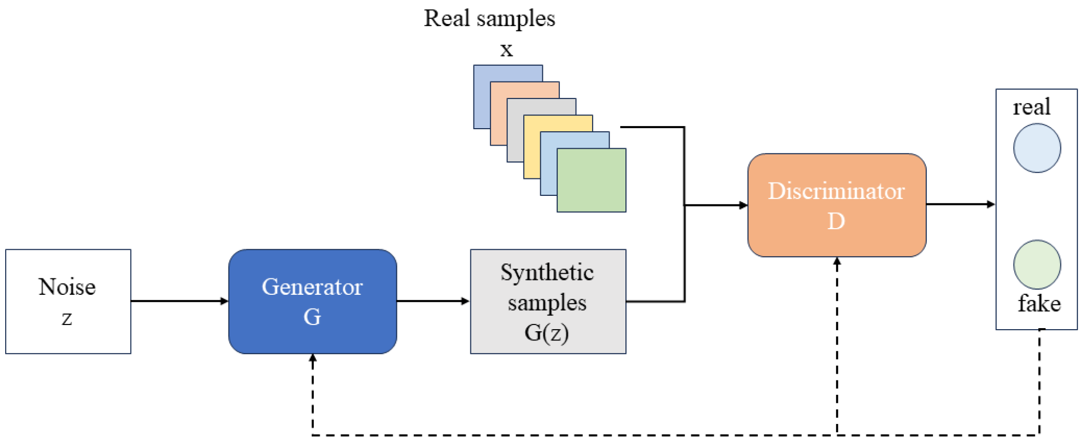
CGANs build upon the original GAN design by incorporating both a generator (G) and a discriminator (D) that compete during training. In the standard GAN setting, illustrated in Figure 1, the generator transforms random noise z through nonlinear mappings to create artificial samples, whereas the discriminator judges each input as real or synthetic and outputs a likelihood score between 0 and 1. This competition forces the generator to improve until the produced data approximate the underlying distribution of real observations.

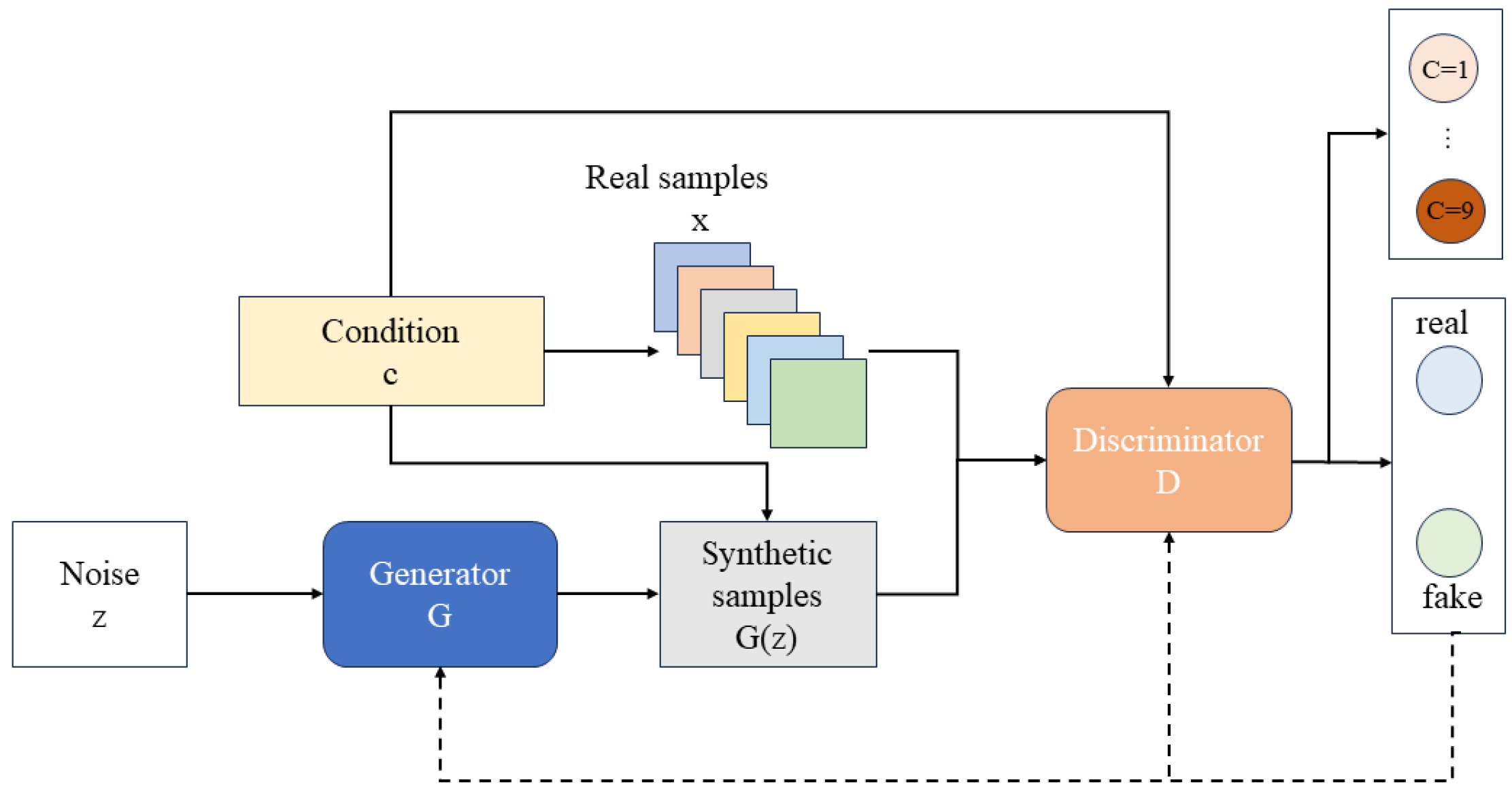
In contrast, CGANs extend this process by adding condition information c into the training pipeline, as shown in Figure 2. The generator receives both the noise vector z and the condition c to produce samples aligned with the specified label, while the discriminator evaluates pairs of samples and conditions together. This additional guidance steers the adversarial learning toward category-consistent outputs. Then, the mathematical form of the CGAN objective function is given below:

$$V(D,G)=\underset{G}{min}\underset{D}{max}({\mathbb{E}}_{x\sim P_{\mathrm{data}}}\left[logD\left(x\right|c)\right]+{\mathbb{E}}_{z\sim P\left(z\right)}\left[log\left(1-D\left(G\right(z\left|c\right))\right)\right])$$

(1)

where $x\sim P_{\mathrm{data}}$ denotes the real samples x following the data distribution, $z\sim P\left(z\right)$ presents the random noise z following the noise distribution input into the generator, E denotes the expected value with respect to the distribution specified in the subscript, and $G\left(z\right)$ denotes the generated samples.

The improved CGAN is constructed using a one-dimensional convolutional neural network based on the traditional CGAN, and its optimization is carried out with the Wasserstein distance. In contrast, the traditional CGAN employs a loss function based on the JS divergence to measure the difference between generated and real samples.

However, the JS divergence presents several limitations during training. First, it provides a weak gradient signal between the generator and discriminator, particularly when the distribution of generated samples differs significantly from that of the true data, which can lead to vanishing gradients. As a result, the generator struggles to learn the underlying data distribution and often suffers from mode collapse, producing only a limited set of samples without capturing the true diversity. Moreover, the JS divergence exhibits instability in high-dimensional settings, which may cause training to become unstable or even fail to converge. Due to these issues and the lack of an effective optimization signal, traditional GANs often perform poorly on complex tasks.

To address these problems, the Wasserstein distance was introduced, leading to the conditional Wasserstein GAN (CWGAN). The Wasserstein distance, derived from optimal transport theory, measures the minimal transport cost between two probability distributions. Compared with the JS divergence, it provides smoother and more informative gradients, stabilizes training, and alleviates the vanishing gradient problem even when the generator–discriminator gap is large. The Wasserstein distance is defined as:

$$W(P_r,P_g)=\underset{\gamma \sim \prod (P_r,P_g)}{inf}{\mathbb{E}}_{(x,y)\sim \gamma }\left[\parallel x-y\parallel \right]$$

(2)

where $P_r,P_g$ represent the distributions of real samples and generated samples, respectively; ${inf}_{\gamma \sim \prod (P_r,P_g)}$ represents the lower bound of the joint probability distribution of real and generated samples. ${\mathbb{E}}_{(x,y)\sim \gamma }[\parallel x-y\parallel ]$ denotes the expected distance between real samples and generated samples.

To address the limitations of JS divergence, this paper employ the CWGAN-GP. The objective function of CWGAN-GP is formulated as the following minimax game:

$$V(G,D)=\underset{G}{min}\underset{D}{max}\{{\mathbb{E}}_{x\sim P_r}\left[D\left(x\right|c)\right]-{\mathbb{E}}_{\tilde{x}\sim P_g}\left[D\left(\tilde{x}\right|c)\right]-\lambda ·{\mathbb{E}}_{\tilde{x}\sim P_g}\left[{\left(\parallel {\nabla }_{\tilde{x}}D\left(\tilde{x}\right|c){\parallel }_2-1\right)}^2\right]\}$$

(3)

where ${\mathbb{E}}_{x\sim P_r}\left[D\left(x\right|c)\right]$ denotes the expected score of real samples conditioned on c. The discriminator aims to maximize this term by assigning higher scores to real samples x. ${\mathbb{E}}_{\tilde{x}\sim P_g}\left[D\left(\tilde{x}\right|c)\right]$ is the expected score of generated samples conditioned on c. The discriminator aims to minimize this term by assigning lower scores to generated samples $\tilde{x}$. $\lambda ·{\mathbb{E}}_{\widehat{x}\sim P_{\widehat{x}}}\left[{\left(\parallel {\nabla }_{\widehat{x}}D\left(\widehat{x}\right|c){\parallel }_2-1\right)}^2\right]$ represents the gradient penalty term, where $\widehat{x}$ is sampled along straight lines between real and generated data points, and $\lambda$ controls the penalty strength. This term enforces the 1-Lipschitz constraint for stable training.

Here, the discriminator D is trained to maximize the value function V by assigning higher scores to real samples and lower scores to generated ones, while simultaneously satisfying the 1-Lipschitz constraint via the gradient penalty. The generator G is trained to minimize V by fooling the discriminator, i.e., by generating samples that receive high scores. The interpolated sample $\widehat{x}$ is defined as $\widehat{x}=ϵx+(1-ϵ)\tilde{x}$, with $ϵ\sim U[0,1]$.

2.2. A Data Augmentation Framework for Data Imbalance

In fault datasets, data imbalance often causes models to favor majority classes and overlook minority features. To mitigate this and address the limitation of convolutional networks applying the same kernel weights to all features, we introduce an attention mechanism into both the generator and discriminator of CWGAN. After noise and label features are concatenated, the attention module adaptively assigns weights to different features, enhancing minority-class representation, improving sample authenticity and diversity, and forming the attention-based conditional Wasserstein GAN (ACW-GAN).

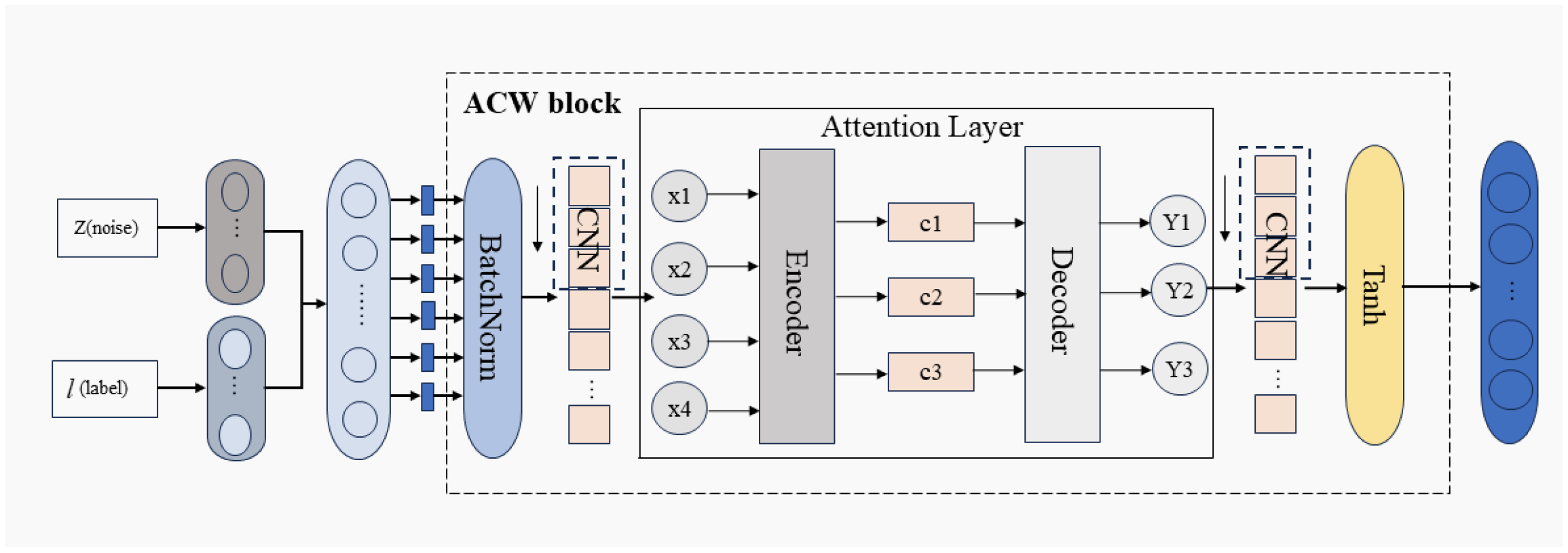
To address the imbalance in one-dimensional fault samples, a generative network is proposed to produce additional fault samples. The overall structure is shown in Figure 3. As illustrated, a random noise z and a class label l are first input into the generator and passed through the attention–convolution–weighting (ACW) module, which mainly consists of one-dimensional convolution and an attention mechanism. Specifically, z and l are concatenated into a long sequence, which is then segmented and normalized using a BatchNorm layer. Local features are extracted through one-dimensional convolution, while global features are captured by the attention mechanism, and the combination of both ultimately produces the generated samples.

The introduction of the attention mechanism enables the network to concentrate on informative feature regions during feature extraction, thereby improving both the quality and the diversity of the generated samples. In the generation process, the random noise vector z and the class label l are concatenated into a long sequence X, which serves as the input data. This sequence is normalized by a BatchNorm layer and subsequently passed through a one-dimensional convolutional layer to extract local patterns, yielding convolutional features

$$C=\mathrm{Conv}1\mathrm{D}\left(X\right).$$

(4)

Since convolution primarily emphasizes local dependencies, an additional attention layer is incorporated to capture global correlations, ensuring that both local and global characteristics are effectively represented. Specifically, the convolutional features C are linearly projected to obtain the query Q, key K, and value V,

$$Q=W_{Q}C,K=W_{K}C,V=W_{V}C,$$

(5)

where $W_Q,W_K,W_V$ denote trainable weight matrices. The attention output is then calculated as

$$\mathrm{Attention}(Q,K,V)=\mathrm{softmax}\left({\displaystyle \frac{Q{K}^T}{\sqrt{d_k}}}\right)V,$$

(6)

and fused with the original convolutional representation to obtain the final feature embedding

$$F=C+\mathrm{Attention}(Q,K,V).$$

(7)

Finally, the fused features F are processed through a fully connected layer to generate synthetic vibration signals $\widehat{x}$. These generated samples, together with authentic fault signals and their category labels, are subsequently passed into the discriminator, which also employs the ACW module. Within this module, one-dimensional convolutional layers are utilized to extract discriminative representations, allowing the discriminator to evaluate whether each input instance corresponds to genuine or artificially generated data.

As shown in Figure 4, the discriminator receives three types of inputs: the synthetic samples $\widehat{x}$, the real signals x, and the associated labels l. These inputs are first passed through an ACW module, which is structurally similar to the generator and composed of one-dimensional convolution and an attention mechanism. The convolutional layers capture local signal characteristics, while the attention mechanism emphasizes global dependencies, yielding the feature representations

$$F_{\widehat{x}}=ACW(\widehat{x},l),F_x=ACW(x,l).$$

(8)

Subsequently, the extracted features are further processed through one-dimensional convolutional layers to obtain compact representations,

$$C_{\widehat{x}}=Conv1D\left(F_{\widehat{x}}\right),C_x=Conv1D\left(F_x\right),$$

(9)

which are then mapped to probability estimates via fully connected layers:

$$p_{real}=FC\left(C_x\right),p_{synthetic}=FC\left(C_{\widehat{x}}\right).$$

(10)

Figure 4. The discriminator for stable adversarial training.

Figure 4. The discriminator for stable adversarial training.

In this manner, the discriminator learns to distinguish authentic signals from synthetic outputs, maximizing the confidence score for real data while minimizing it for generated data. Once the adversarial training converges to a Nash equilibrium, only synthetic signals of sufficient quality are retained and combined with real measurements, thereby enriching the dataset. On this basis, the loss function of the discriminator, denoted as $L_D$, can be formulated as:

$$L_D={\mathbb{E}}_{\tilde{x}\sim P_g}\left[D\left(\tilde{x}\right|l)\right]-{\mathbb{E}}_{x\sim P_r}\left[D\left(x\right|l)\right]+\lambda ·{\mathbb{E}}_{\widehat{x}\sim P_{\widehat{x}}}\left[{\left(\parallel {\nabla }_{\widehat{x}}D\left(\widehat{x}\right|l){\parallel }_2-1\right)}^2\right]$$

(11)

where ${\mathbb{E}}_{\tilde{x}\sim P_g}\left[D\left(\tilde{x}\right|c)\right]$ denotes the expected score of generated samples conditioned on c. The discriminator aims to minimize this term by assigning lower scores to generated samples $\tilde{x}$. ${\mathbb{E}}_{x\sim P_r}\left[D\left(x\right|c)\right]$ is the expected score of real samples conditioned on c. The discriminator aims to maximize this term (by minimizing its negative) by assigning higher scores to real samples x. $\lambda ·{\mathbb{E}}_{\widehat{x}\sim P_{\widehat{x}}}\left[{\left(\parallel {\nabla }_{\widehat{x}}D\left(\widehat{x}\right|c){\parallel }_2-1\right)}^2\right]$ represents the gradient penalty term that ensures the discriminator satisfies the 1-Lipschitz continuity condition, where $\widehat{x}=ϵx+(1-ϵ)\tilde{x}$ with $ϵ\sim \mathrm{Uniform}[0,1]$ is a randomly interpolated sample between real and generated data.

The generator is designed to create synthetic data that closely resemble real samples, thereby reducing the ability of the discriminator to tell them apart. The corresponding loss function of the generator, denoted as LG, is expressed as:

$$L_G=-{\mathbb{E}}_{\tilde{x}\sim P_g}\left[D\left(\tilde{x}\right|l)\right]$$

(12)

where $-{\mathbb{E}}_{\tilde{x}\sim P_g}\left[D\left(\tilde{x}\right|c)\right]$ denotes the negative expected score of generated samples conditioned on c. The generator aims to minimize this loss by producing samples $\tilde{x}$ that receive high scores from the discriminator, thereby fooling the discriminator into classifying generated samples as real.

During the training process, both the generator and discriminator are updated in opposition to each other. The generator focuses on producing highly realistic data, whereas the discriminator enhances its capability to correctly identify authenticity. Once the two networks reach a state of Nash equilibrium, the generator is able to synthesize data whose distribution is nearly indistinguishable from that of the real samples, which lays the foundation for the subsequent fault diagnosis framework.

3. Enhanced Fault Diagnosis via Augmentation and Wavelet–ResNet

In actual industrial processes, mechanical equipment generally operates under normal conditions, and fault data are often scarce. This scarcity leads to an imbalance in the training dataset and limits the effectiveness of fault diagnosis models. To address this issue, we propose a fault diagnosis learning framework under data imbalance conditions, which integrates the ACW-GAN–based data augmentation approach developed in Section 2 with a wavelet–ResNet classifier. The ACW-GAN enhances the quality and diversity of synthetic samples, thereby expanding the original imbalanced dataset, while wavelet transform and ResNet improve feature extraction and classification performance.

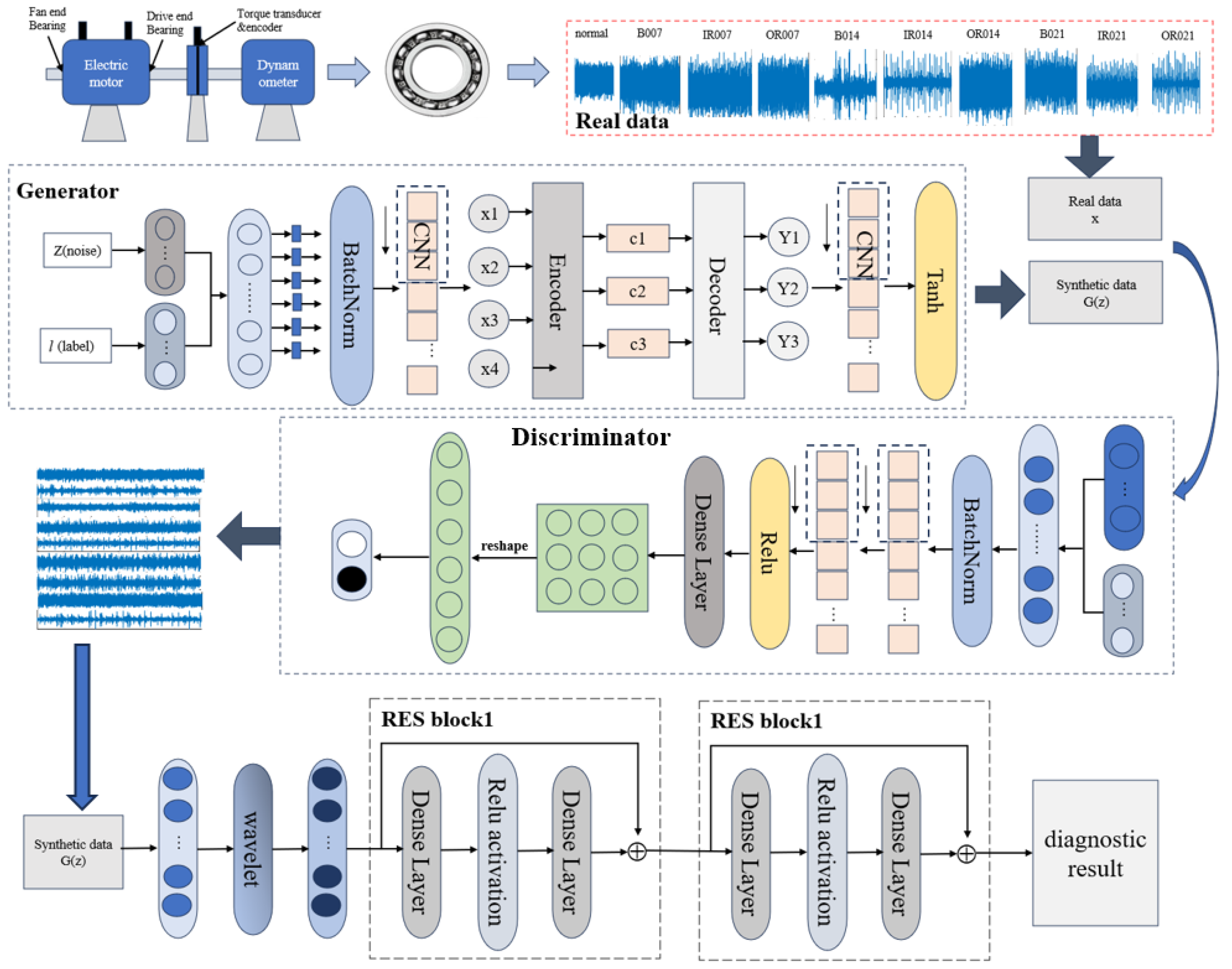
As illustrated in Figure 5, the overall framework consists of four components: (1) Data acquisition: one-dimensional vibration signals under different fault conditions are collected by accelerometers as real samples; (2) Data augmentation: limited fault samples are normalized and fed into the ACW-GAN to generate high-quality synthetic data; (3) Synthetic sample quality assessment: o evaluate the quality of generated samples in the frequency domain, Fast Fourier Transform (FFT) is applied to obtain their frequency spectra. For the fault diagnosis model, however, wavelet transform is employed to extract time-frequency representations from the vibration signals, providing joint time and frequency information crucial for identifying non-stationary fault characteristics; (4) Fault diagnosis model training: synthetic and real data are used to train the wavelet–ResNet model, where wavelet transform extracts time–frequency fault features and ResNet mitigates gradient vanishing issues, leading to reliable fault diagnosis.

Since the first two steps were addressed in Section 2, this section focuses on the latter two components, beginning with an introduction to the ResNet framework.

3.1. Residual Network Architecture

Deep Convolutional Neural Networks (CNNs) have demonstrated strong feature learning capabilities, but as network depth increases, they encounter serious challenges such as gradient vanishing, gradient explosion, high computational cost, and overfitting. These issues hinder effective parameter optimization and limit the performance of very deep models in practice.

To address these difficulties, He et al. [40] proposed the ResNet, which introduces the concept of residual learning. The key idea is to reformulate the mapping to be learned as a residual function, where identity mappings (skip connections) are added to traditional convolutional layers. This simple yet powerful design facilitates error backpropagation, stabilizes gradient flow, and significantly improves the optimization of deep neural networks.

Structurally, ResNet consists of an input stage, a series of convolutional layers with batch normalization (BN), residual blocks with shortcut connections, a global average pooling layer, and a final fully connected output stage. The core component is the residual block, in which the output of a sequence of operations (BN → ReLU → Conv → BN → ReLU → Conv) along the main path is added element-wise to the shortcut (identity mapping). This additive fusion enables the network to directly propagate information across layers, effectively mitigating the degradation problem in deep CNNs. As illustrated in Figure 6, this residual learning mechanism allows ResNet to maintain accuracy even as depth increases.

By integrating identity mappings into convolutional architectures, ResNet not only alleviates gradient degradation but also enhances training stability and convergence efficiency. These properties have contributed to its wide adoption in computer vision tasks and, in this study, make it a suitable backbone for fault diagnosis, where robust feature extraction and stable optimization are essential.

3.2. Wavelet-Enhanced ResNet for Fault Diagnosis

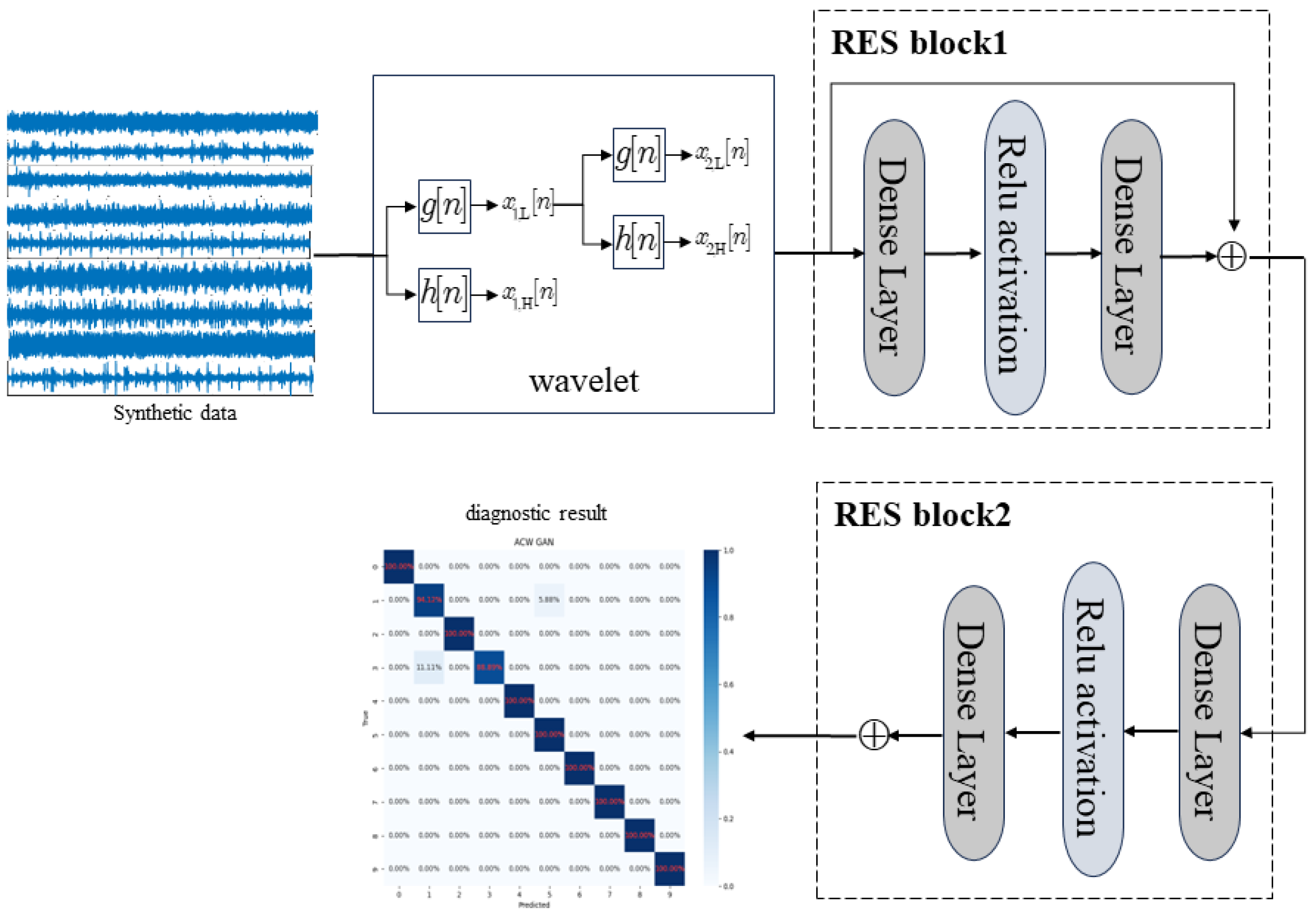
Building on this backbone, we further integrate wavelet transform with ResNet to construct the fault diagnosis model. Wavelet transform provides complementary time–frequency information, which enhances the feature extraction capability of ResNet and enables more accurate recognition of non-stationary fault signals. The overall ResNet-based fault diagnosis framework is illustrated in Figure 7.

To achieve a more comprehensive signal analysis in both the time and frequency domains, this study employs wavelet transform. Purely temporal analysis considers only variations along the time axis and fails to capture fault characteristics concentrated in specific frequency bands. Moreover, fault signals are typically non-stationary, making time-domain methods alone insufficient. Wavelet transform addresses these issues by decomposing signals into a linear combination of wavelet basis functions, which effectively describe local features. By adjusting scale and position, the transform can capture frequency components and locate their evolution across multiple time scales.

Within the proposed diagnostic framework, the synthesized fault data generated by ACW-GAN is first subjected to wavelet decomposition to obtain detailed time–frequency representations. These feature maps are then fed into a multi-layer ResNet to perform deep representation learning and accurate fault recognition. Through adversarial training, the quality of generated samples is progressively enhanced until Nash equilibrium is reached, ensuring reliable synthetic data for training. The final augmented dataset undergoes wavelet transformation to provide the time–frequency representations required for effective fault diagnosis.

$$W_{\psi }\left(x\right)(a,b)={\int }_{-\infty }^{+\infty }x\left(t\right){\displaystyle \frac{1}{\sqrt{a}}}\psi \left({\displaystyle \frac{t-b}{a}}\right)dt$$

(13)

where $\psi$ represents the mother wavelet function, a and b denote the scale and translation parameters, respectively. Subsequently, a residual network with multiple layers is employed, into which the wavelet-derived features are introduced for advanced representation learning and fault classification. By incorporating shortcut connections, ResNet effectively mitigates the gradient vanishing issue that often arises in very deep architectures. Each residual block includes a skip connection, allowing the direct passage of input to the output, which facilitates better training and optimization of the network.

4. Case Study Analysis of the Bearing Experiment

4.1. Experimental Setup and Data Preprocessing

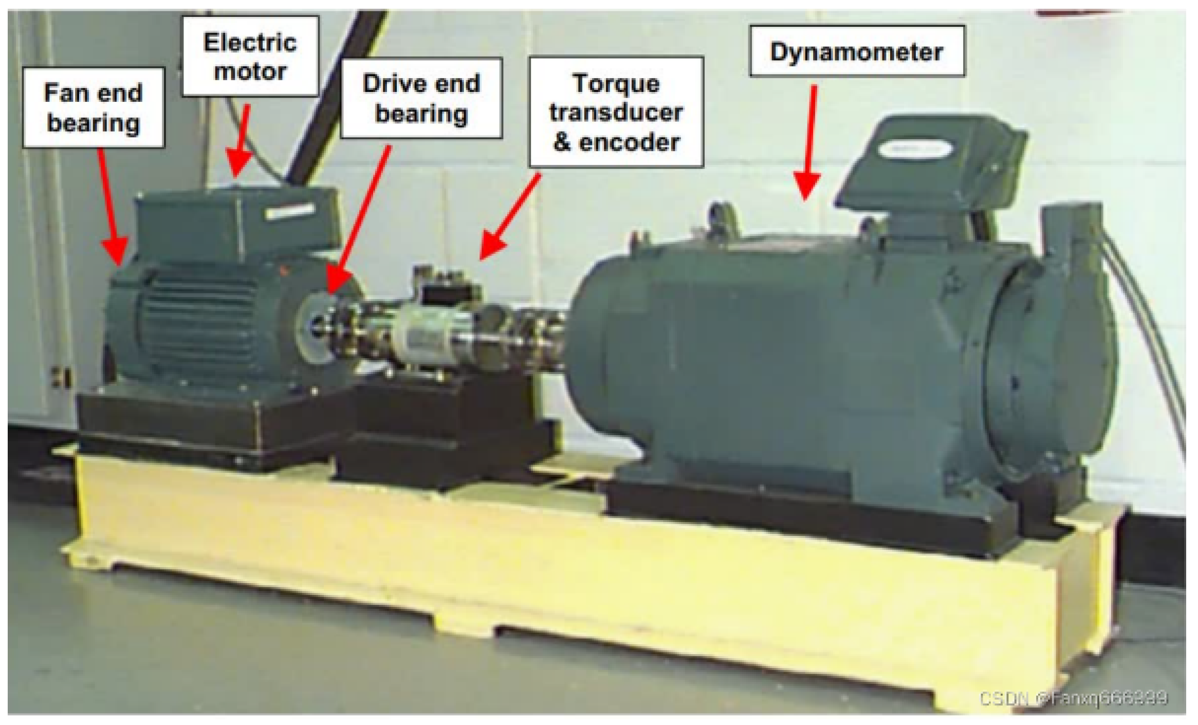
To validate the effectiveness and superiority of the ACW-based enhanced diagnostic method proposed in this study, experimental verification is conducted using the CWRU bearing dataset [41]. The experimental platform for the CWRU bearing dataset, as shown in Figure 8, primarily consists of a motor, torque sensor, dynamometer, and electronic controller. This bearing dataset includes data from actual damaged bearings, which realistically reflects the complexity of real-world bearing data and effectively verifies the applicability of the proposed method in practical industrial scenarios.

In the experiments, vibration signals were recorded from the drive end of an induction motor running at 1797 rpm with no external load. Data acquisition was performed at a sampling rate of 12 kHz, and each individual record contained 1200 consecutive points without overlap. To create a training set suitable for evaluation, the dataset was deliberately constructed with a 75% imbalance ratio.

The test bench was capable of replicating both healthy and defective bearing conditions. Accelerometers were mounted on the bearing housing to capture the corresponding vibration responses. Four operating states were investigated: a normal condition (NOR), inner race damage (IF), outer race damage (OF), and ball defects (BF). Artificial faults with diameters of 0.007, 0.014, and 0.021 inches were introduced, producing one healthy category and nine distinct fault categories in total, as summarized in

Table 1. Fault Categories.

Fault State	Size (in)	Training Set		Test Set	Class Label
		Original	Generated
Normal	0	100	0	20	0
Inner fault	0.007	40	60	20	1
	0.014	40	60	20	2
	0.021	40	60	20	3
Outer fault	0.007	40	60	20	4
	0.014	40	60	20	5
	0.021	40	60	20	6
Ball fault	0.007	40	60	20	7
	0.014	40	60	20	8
	0.021	40	60	20	9

.

4.2. Quality Assessment of the Generated Samples

Before assessing the quality of the generated samples, it is essential to first evaluate their diversity. To this end, the original one-dimensional vibration signals are transformed into two-dimensional grayscale images, which provide a more intuitive visualization of time-domain characteristics such as waveform shape, periodicity, and randomness. Grayscale representations also highlight the frequency and amplitude distributions of the signals, where variations in brightness and density reflect differences in these characteristics.

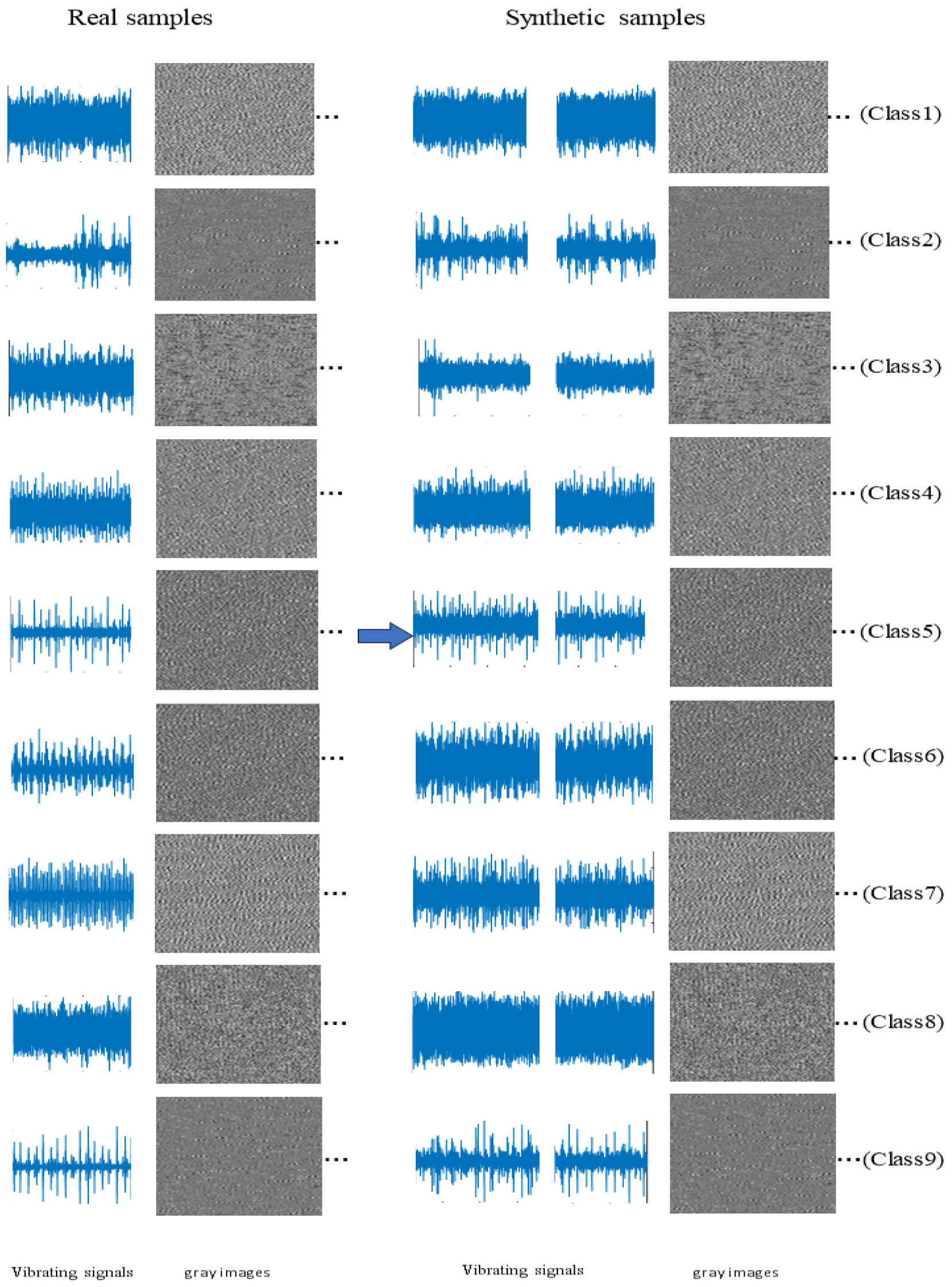
A generative model with good diversity produces signals exhibiting varied waveform patterns, frequencies, and amplitudes, which are clearly distinguishable in the corresponding grayscale images. As shown in Figure 9, the generated fault signals across different categories display distinct image patterns compared with the original samples, demonstrating that the proposed GAN-based method successfully captures category-specific diversity.

To demonstrate the advantages of the proposed approach, this section presents a qualitative evaluation of the generated samples along with a comparative study against alternative models.

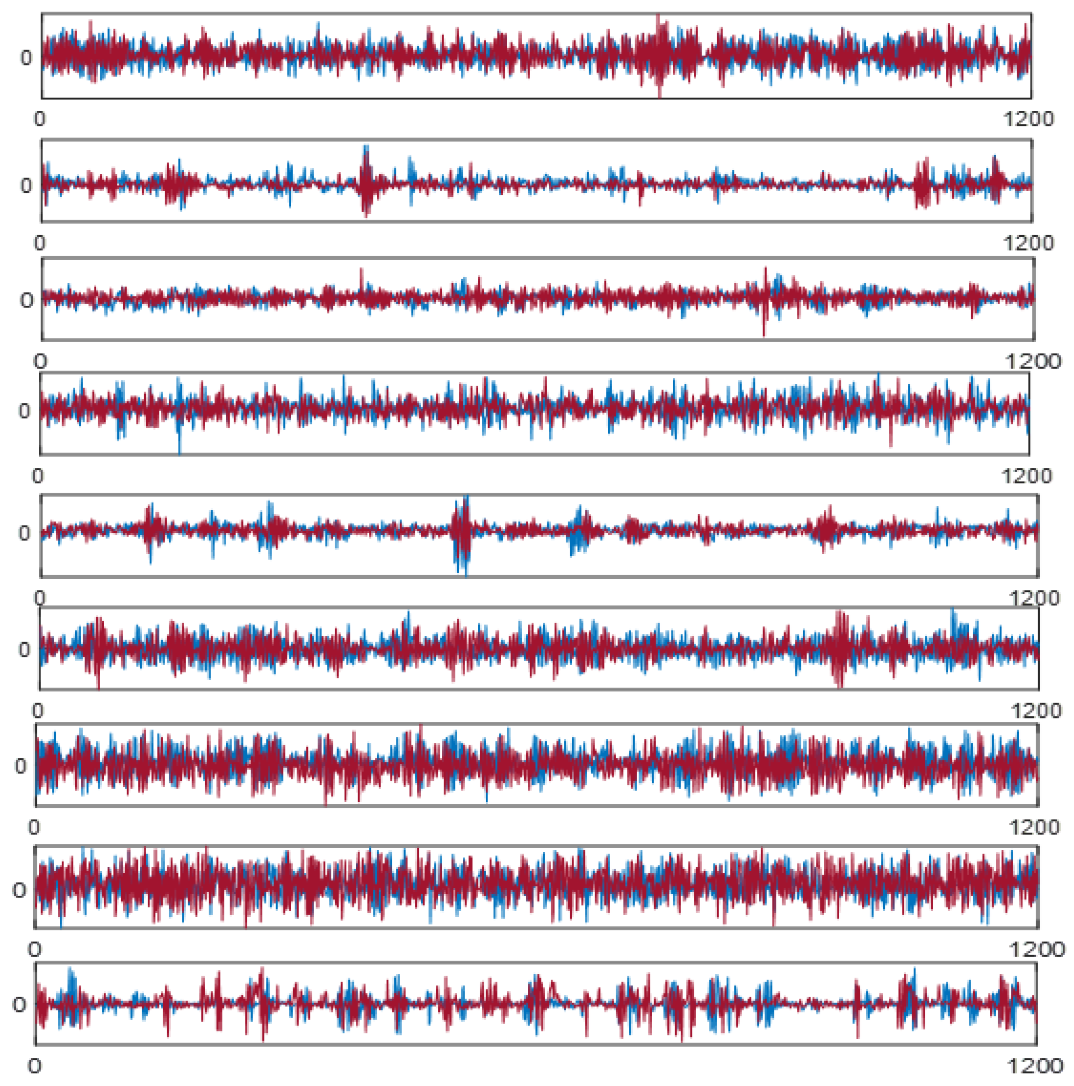
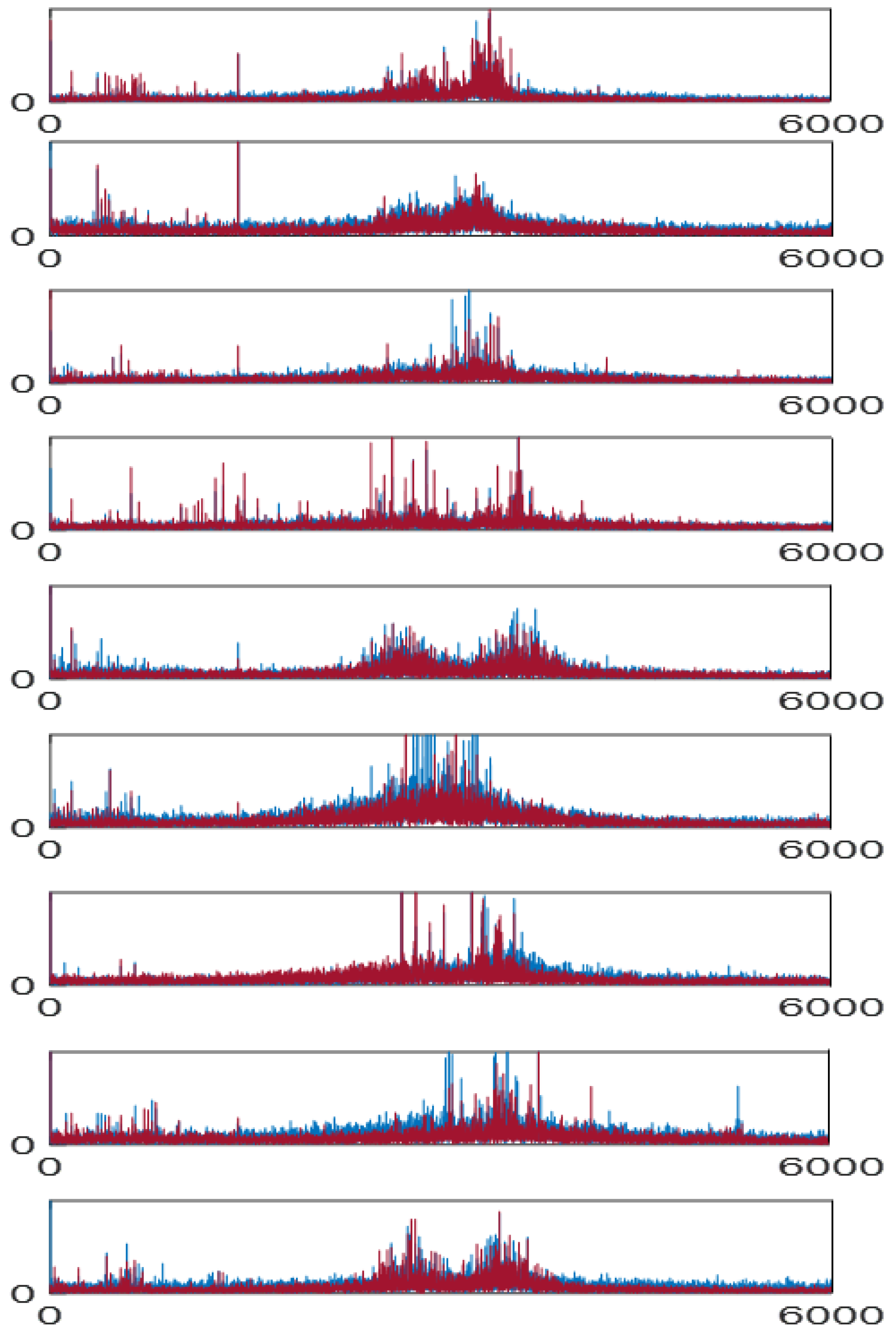
Evaluating the quality of the generated data is essential for assessing its consistency with the original dataset. To this end, signals are examined in both the time and frequency domains to identify potential discrepancies. Nine categories of experimental data were selected, with their time-domain and frequency-domain representations shown in Figure 10 (where the x-axis represents sampling points and the y-axis represents normalized amplitude) and Figure 11 (where, the x-axis is now marked as frequency (Hz), and the y-axis is marked as amplitude), respectively. In these figures, the generated data are plotted in red and the original data in blue.

In the time-domain representation, each curve consists of 1200 sampled points, with the horizontal axis denoting the sequence index and the vertical axis showing the normalized amplitude. For spectral analysis, the signals are transformed using FFT at a sampling rate of 12 kHz, where the abscissa corresponds to frequency and the ordinate to relative amplitude. Every subplot in Figure 10 and Figure 11 is associated with one of the bearing conditions summarized in Table 1. Figure 10 illustrates that the generated samples exhibit temporal patterns that are highly consistent with those of the original signals. Likewise, Figure 11 reveals that the frequency characteristics are faithfully reproduced. The frequency range is limited to 6000 Hz according to the Nyquist theorem, given the 12 kHz sampling rate. demonstrating that the model is capable of producing synthetic signals that retain both temporal and spectral integrity.

These observations verify that the method successfully models the true data distribution and produces realistic fault examples. Such synthetic data can be effectively integrated into the training set to enhance classification performance. Taken together, the visual comparisons confirm the close correspondence between generated and actual signals across different fault categories, underscoring the reliability and high quality of the generated dataset.

4.3. Fault Diagnosis Analysis Based on the Proposed Method

The proposed fault diagnosis approach consists of three main parts: generator, discriminator, and residual network. The specific model details are listed in

Table 2. Network Model Structure and Parameters.

Module	Network Structure	Network Parameters
Generator	Dense_1	Output units = 256, activation = ReLU
	Conv1D_1	Channels = 128, kernel size = 3, stride = 1, activation = ReLU
	Dense_2	Output units = 256, activation = ReLU
	Concatenate	Output shape = (1, 512)
	Attention	Activation = Sigmoid
	Conv1D_2	Channels = 64, kernel size = 3, stride = 1, activation = ReLU
Discriminator	Conv1D_1	Channels = 64, kernel size = 3, stride = 1, activation = ReLU
	Conv1D_2	Channels = 128, kernel size = 3, stride = 1, activation = ReLU
	Dense	Output units = 1, activation = Sigmoid
ResNet	Conv1D_1	Channels = 64, kernel size = 3, stride = 1, activation = ReLU
	Conv1D_1-1	Channels = 64, activation = ReLU
	Conv1D_2	Channels = 64, kernel size = 3, stride = 1, activation = ReLU
	Conv1D_2-1	Channels = 64, activation = ReLU
	Conv1D_3	Channels = 64, kernel size = 3, stride = 1, activation = ReLU
	Conv1D_3-1	Channels = 64, activation = ReLU
	Dense	Output units = 128, activation = ReLU

.

To verify the capability of ACWGAN in mitigating class imbalance for fault diagnosis, experiments were carried out using ten different datasets. In addition, ablation analyses were designed to investigate the role of specific modules in the framework. The study focused on two main aspects: the effect of embedding an attention mechanism into the CGAN to enhance the fidelity of generated samples, and the replacement of the traditional JS divergence with the Wasserstein distance to achieve a more accurate distinction between real and artificial data. A summary of the ablation variants and their corresponding diagnosis outcomes is provided in

Table 3. Ablation experiments.

Model	Attention Mech	CGAN	Wasserstein	ResNet	Result
ACWGAN	✓	✓	✓	✓	100%
CWGAN		✓	✓	✓	94%
ACGAN	✓	✓		✓	92%
GAN				✓	86%

. Three variants were considered: (i) removing the attention mechanism, (ii) removing the Wasserstein distance, and (iii) removing the GAN-based data augmentation component.

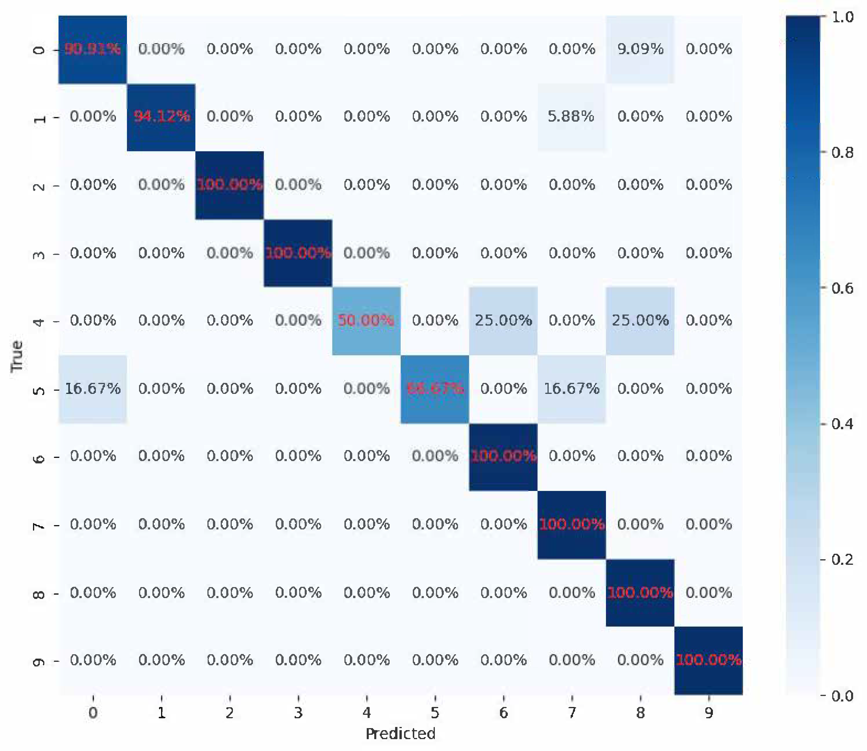
From the table above, one can see that the fault diagnosis accuracy of the proposed ACWGAN method is 100%, higher than the other ablation experiments. This proves the superiority of ACWGAN in fault diagnosis when combined with the attention mechanism and Wasserstein distance. To further illustrate the differences of the models, a confusion matrix is constructed in Figure 12.

As shown in Figure 12a, the proposed ACWGAN achieves a fault diagnosis accuracy of 100%, demonstrating the superiority of the method. The ablation studies in Figure 12b–d further highlight the contributions of individual components. Figure 12b illustrates that the attention mechanism improves the ability of the model to capture global features of vibration signals. Without attention, only local features are emphasized, resulting in less detailed synthetic data that cannot adequately represent real fault characteristics. Figure 12c confirms that replacing JS divergence with Wasserstein distance enhances the ability of the discriminator to measure distribution differences between real and generated data, thereby improving the fidelity of synthetic samples. In contrast, the JS-based approach reduces distribution matching and leads to lower diagnosis accuracy. Figure 12d shows that introducing conditional information into the GAN enables the generation of category-specific fault samples, improving both diversity and quality. Without conditioning, the generated data fail to capture label information effectively, decreasing diagnostic performance.

To further demonstrated the proposed fault diagnosis method, a comparative experiment is conducted using traditional CNNs and ResNets for fault diagnosis. Both models were trained with high-quality synthetic samples generated by ACWGAN, and their classification performance was evaluated on the same dataset. The confusion matrix of the CNN-based fault diagnosis results is presented in Figure 13.

Experimental results demonstrated that the ResNet model outperformed conventional CNN models in fault diagnosis tasks. Specifically, by introducing residual blocks, ResNet was able to capture deeper hierarchical features from the input data. Compared with traditional CNNs, ResNet exhibited a stronger capability in extracting features from complex fault signals, making it more effective in identifying fault patterns. Deep neural networks were prone to gradient vanishing problems, which made training difficult. ResNet alleviated this issue through skip connections, enabling more effective training and optimization of deep networks and thereby improving overall model performance. The comparative experiments indicated that the ResNet model achieved higher detection accuracy and stronger feature extraction capability in fault diagnosis, validating the effectiveness and superiority of employing ResNet in this study. When combined with high-quality samples generated by the ACWGAN, the ResNet model provided more reliable and accurate detection results for fault diagnosis.

5. Conclusions

This paper proposes a fault sample enhancement method based on ACWGAN and a fault diagnosis framework that combines wavelet decomposition with ResNet, aiming to improve diagnostic accuracy and alleviate data imbalance. This method first adopts a generative adversarial network constructed by one-dimensional convolution and attention mechanism. We evaluated the quality of generated data by comparing time and frequency domains and trained diagnosis models using only high-quality synthesized samples. For fault diagnosis, wavelet decomposition extracts time-frequency features from vibration signals, while ResNet performs deep feature learning and classification.

The proposed method has been validated using the CWRU bearing dataset, which contains real fault data representing actual operating conditions. The experiment involves evaluating the diversity and quality of generated data. In order to conduct diversity assessment, one-dimensional vibration signals are converted into two-dimensional grayscale images, where changes in shape and density indicate satisfactory diversity. To conduct quality assessment, FFT is applied to compare the spectral characteristics of the generated and original samples. The results indicate that the distribution of synthesized data and real data in both domains is very close, confirming their high fidelity. In order to verify the robustness of the proposed method, ablation and comparative experiments were conducted. The ablation study, in turn, eliminated attention mechanisms, Wasserstein distance, and GAN components, each of which resulted in a decrease in diagnosis accuracy, highlighting the importance of these elements. The comparative experiment with traditional CNN proves the superior performance of ResNet combined with wavelet decomposition.

Although the proposed ACWGAN–Wavelet–ResNet framework demonstrates excellent performance in bearing fault diagnosis, certain limitations remain. First, the model was validated primarily on the CWRU bearing dataset, and its generalization capability to other types of mechanical systems requires further investigation. Second, the attention-enhanced GAN and wavelet–ResNet structures increase model complexity, which can limit real-time applicability in large-scale industrial monitoring. Additionally, the framework relies on a sufficient amount of labeled fault data to guide conditional generation, which may be challenging to obtain in some industrial scenarios. In future work, we will explore lightweight network architectures and transfer learning techniques to improve computational efficiency and cross-domain adaptability. Moreover, the extension of the proposed framework to multimodal signals and real-time monitoring environments will be a key focus to further enhance its industrial scalability.