Abstract
The surface transportation of heavy crude oil remains an operational challenge due to its high viscosity and rapid heat loss when exposed to ambient conditions, which significantly increases the energy required for pumping. Although previous studies have estimated thermal losses using average convective coefficients, they have not characterized the internal development of the thermal and velocity boundary layers, nor their direct influence on viscosity and flow regime. The objective of this study is to develop a predictive model based on computational fluid dynamics with temperature-dependent properties, enabling the analysis of the interaction between heat transfer phenomena and flow dynamics along a 50 m SCH-80 pipeline segment under real conditions of the Ecuadorian Oriente and to propose a mathematical tool capable of accurately predicting temperature loss over long pipeline sections. The results show a temperature decrease from 346.5 K to 342.5 K, accompanied by the formation of a thermal boundary layer that reaches 87% of the pipe radius and a reduction in the Reynolds number to approximately 5 due to the increase in viscosity. Furthermore, an effective external convective heat transfer coefficient of 5 W·m−2·K was determined, and the developed polynomial model achieved a coefficient of determination R2 of 0.998, confirming its predictive capability for optimizing the transportation of heavy crude oils.
1. Introduction
The exploitation and transportation of heavy crude oil pose significant challenges for the petroleum industry due to its high density and viscosity, which are characteristic of low-API gravity crudes [1,2]. These properties hinder flow through pipelines and require a higher energy input for pumping, thereby increasing operational costs and reducing process efficiency [3]. Several studies have proposed crude oil heating techniques to reduce its viscosity through the application of thermal or electromagnetic methods [4,5], demonstrating that the increase in temperature substantially enhances fluid mobility. However, most of these studies have focused on downhole or reservoir heating processes, while the phenomenon of heat loss during surface transportation has received less attention, despite being a determining factor in the increase in viscosity and the reduction in the hydraulic performance of the system [6,7]. Moreover, recent studies have demonstrated that the use of viscoelastic polymers and the control of reservoir wettability can significantly enhance heavy crude oil recovery by improving its mobility and reducing residual capillary trapping [8]. These advancements confirm that the thermo-hydraulic analysis developed in this study constitutes a fundamental step toward integrating transportation and enhanced oil recovery strategies, strengthening operational efficiency from the surface flow phase to the displacement stage within the reservoir.
The decrease in temperature during the surface transport of crude oil represents a critical technical challenge due to the significant increase in crude viscosity as its temperature drops [9]. This increase in viscosity causes greater resistance to flow within the pipelines, which requires higher pressure and pumping power to maintain an adequate flow rate. This condition increases the workload on pumping equipment and can lead to reduced transport efficiency, raising the risk of deposit formation and blockages that may obstruct the pipelines. In addition, the higher viscosity of the crude can cause accelerated wear on the components of the transport system, increasing operating and maintenance costs. To mitigate these problems, it is essential to implement thermal control strategies, such as the use of effective thermal insulation and heating systems, to maintain the crude oil temperature within an optimal range that promotes smoother and more efficient flow along the transport infrastructure.
To understand the behavior of heavy crude oil under various operating conditions, multiple studies have been conducted using computational fluid dynamics. These investigations are crucial for optimizing extraction and transport processes, as well as for predicting the operational challenges associated with this type of crude. One such study is that of Cazorla and J. (2013) [10]; they evaluated the impact of applying electromagnetic waves in extra-heavy crude oil reservoirs through horizontal wells. Their objective was to increase production and the recovery factor using an electromagnetic heating system, which allows for the reduction in the high viscosity of extra-heavy crude. To achieve this, numerical simulations were carried out by coupling an electromagnetic model with a reservoir model, using the CERES and STARS programs.
Tolentino et al. (2016) [11] proposed a new alternative for heating heavy and extra-heavy crude oil reservoirs in Venezuela through nuclear reaction capsules that generate heat, with a conceptual design of 152.4 mm in diameter and 3.048 m in length, installed vertically in the porous medium of the reservoir. Their objective was to reduce crude viscosity and improve its mobility to facilitate extraction. Computational simulations were carried out using COMSOL Multiphysics (https://ve.scielo.org/scielo.php?script=sci_arttext&pid=S1316-48212016000200001&lng=es&nrm=iso&tlng=es, accessed on 15 August 2025) under steady-state conditions, without considering the movement of crude oil or trapped fluid, and the results showed the temperature gradient distribution around the capsules in different arrangements.
On the other hand, Saleh et al. (2021) [12] developed a Computational Fluid Dynamics model based on rheology to predict the flow characteristics of Iraqi heavy crude oil through a horizontal pipeline. A power-law rheological model was used to describe the dilatant non-Newtonian behavior of heavy crude oil. Their study focused on predicting velocity profiles, friction factor, wall shear stress, and entry length of heavy crude oil flow through the horizontal pipeline.
Zhang et al. (2022) [13] focused on the three-dimensional numerical simulation of heat transfer and paraffinic crude oil flow in inclined pipelines using CFD software (https://www.sciencedirect.com/science/article/pii/S2214157X2200483X?via%3Dihub, accessed on 15 August 2025). pipelines with inclination angles of 0°, 25°, and 45° were examined, analyzing the temperature and velocity fields of the paraffinic crude, as well as the gelling behavior during crude cooling. Their study identified that natural convection influenced by gravity plays a crucial role in the decrease in temperature along the pipeline inclination. The results showed that increasing the inclination angle causes a greater temperature difference between the highest and lowest points of the pipeline and increases the liquid volume fraction, with the lower sections of the pipeline being more prone to blockages due to crude gelling.
Ramírez et al. (2023) [6] carried out a prediction of temperature and viscosity profiles in heavy oil production wells using a downhole induction heater, with the aim of improving crude mobility by reducing its viscosity through electrical heating. Using a simplified CFD model, validated with experimental data from, an agreement of 0.8% for temperature and 15.69% for viscosity was achieved. The results showed an effective reduction of 46.1% in the dynamic viscosity of heavy crude with heating, although thermal effects in the reservoir were insignificant. This confirms the effectiveness of the enhanced oil recovery (EOR) thermal technique in heavy crude wells, suggesting the need for further studies to explore improvements in energy efficiency and the impact of heating on well productivity.
Kumar R et al. (2023) [14] focused on analyzing heat transfer and flow characteristics in an annular pipeline system transporting crude oil and water, using CFD simulation. A 3D model with high-quality meshes was developed, and boundary conditions were established to study fluid interaction and pressure gradients. The results showed a significant improvement in heat transfer efficiency and a reduction in energy consumption when using nanocomposite heat exchangers. An effective mixing of hot crude and cold water was observed, which optimized the thermal control of the system, with future research proposed on the mixing of bio-nanoparticles with crude and the use of sensors to enhance results.
Although computational fluid dynamics has been widely used to explore the behavior of heavy crude oil under various conditions, there is a notable gap in the scientific literature regarding heat losses at the surface. Existing research has provided a detailed understanding of aspects such as viscosity and crude flow pressure; however, the phenomenon of thermal dissipation during surface transport has been left relatively unexplored. This aspect is crucial for the design of more efficient pumping and pipeline systems, where temperature management can significantly influence the energy efficiency and operational integrity of the system.
Cabrera J et al. (2024) [15] evaluated the temperature loss during the surface pumping of heavy crude oil with an API gravity of 17.5 in the Ecuadorian Oriente, using CFD simulation to analyze a 50 m section of SCH-80 pipeline with a 4-inch diameter. A convective coefficient of 52 W/m2·K and a temperature loss of 3.2 K were determined, providing key information to optimize the transport of heavy crude and explore heating technologies that help maintain its proper viscosity during transportation.
Although the study by Cabrera J et al. (2024) [15] examined crude oil temperature loss in a pipeline section, it is necessary to conduct new research due to the denser and more viscous nature of crude with an API gravity of 11.2, compared to the API 17.5 crude in the aforementioned investigation. Heavier crude presents greater challenges for transportation because of its high viscosity, which further increases with heat loss during surface flow. This type of crude requires deeper analysis to understand how variable viscosity affects flow dynamics and heat transfer in the pipeline—critical factors for designing more efficient transport strategies. This research addresses a critical gap in the state of the art by quantifying, for the first time under real operational conditions in the Ecuadorian Oriente, the development of the thermal and velocity boundary layers in the surface transportation of heavy crude oil—phenomena that govern the progressive loss of temperature, the significant increase in viscosity, and, consequently, the rise in the pumping energy required. Unlike previous studies that are limited to estimating average convective coefficients or bulk thermal losses, this work introduces an innovative approach based on CFD modeling with temperature-dependent properties, enabling axial-resolution characterization of how the expansion of the thermal boundary layer reduces the heat transfer rate and how the thickening of the velocity boundary layer slows down the flow. Additionally, a second-degree predictive polynomial model is developed to capture the nonlinear cooling behavior of the crude along the pipeline, constituting a high-value scientific tool for anticipating critical transport lengths and designing thermal and hydraulic maintenance strategies tailored to low-API crudes, thus providing an unprecedented foundation to optimize operational efficiency and reduce energy costs in the petroleum industry.
2. Materials and Methods
CFD simulation is extensively used in the industry, standing out for its numerous advantages. Among these, the low cost compared to experimental techniques and the ability to model complex physical phenomena are particularly noteworthy [16]. However, it is crucial to experimentally validate the CFD simulation to ensure that the model setup and the selected parameters are appropriate for the specific case study. This validation is essential to confirm the accuracy of the results obtained [17]. Computational fluid dynamics has been widely used in the study of processes in which mass and heat transfer occur in air [18,19].
CFD simulation has become an essential tool in the industry due to its multiple advantages. One of its main strengths is the relatively low cost compared to traditional experimental techniques, which allows for detailed analyses without the need to invest in expensive physical equipment or face the risks associated with field testing [16]. In addition, CFD has the ability to model complex physical phenomena, such as heat transfer, the behavior of non-Newtonian fluids, and the interaction between multiple phases, which would be difficult to accurately replicate through experimental methods. However, to ensure that simulations are reliable and representative of reality, it is essential to perform experimental validation. This involves comparing the simulation results with data obtained from physical tests, which ensures that the chosen models and parameters are appropriate for the specific case study. Validation not only confirms the accuracy of the model, but also allows for adjustments and optimization of the simulation to improve the fidelity of the results [17]. CFD has proven to be especially valuable in the study of processes involving mass and heat transfer, standing out as a versatile tool for optimizing complex industrial operations [18,19].
2.1. Geometry Modelling and Mesh Generation
In the current research, the model used in the simulation maintains the same dimensions as the real pipeline employed in the case study, in Figure 1, the model used can be observed, while the properties of the pipeline and the heavy crude oil can be seen in Table 1.

Figure 1.
Model used in the simulation.

Table 1.
Thermal properties of the pipe and heavy crude.
The CFD simulation model was designed to faithfully reflect the dimensions of the pipeline used in the case study, ensuring that the results obtained are as close as possible to the actual behavior of the system. This geometric accuracy is crucial for properly capturing the physical phenomena involved, such as temperature distribution, velocity profiles, and the interactions between the crude oil and the pipeline walls. It also enables an accurate evaluation of heat transfer and the development of the thermal and velocity boundary layers, which are fundamental factors in the analysis of heavy crude transport.
The viscosity of heavy crude oil can be characterized in two ways: dynamic viscosity and kinematic viscosity, both fundamental for flow modeling in transport systems. dynamic viscosity, as shown in Figure 2, represents the internal resistance of the fluid to displacement when a shear force is applied, being critical for calculating pressure drop and the pumping power required. Furthermore, in Figure 2, a comparison can be observed between the data obtained experimentally and the model from Equation (9).
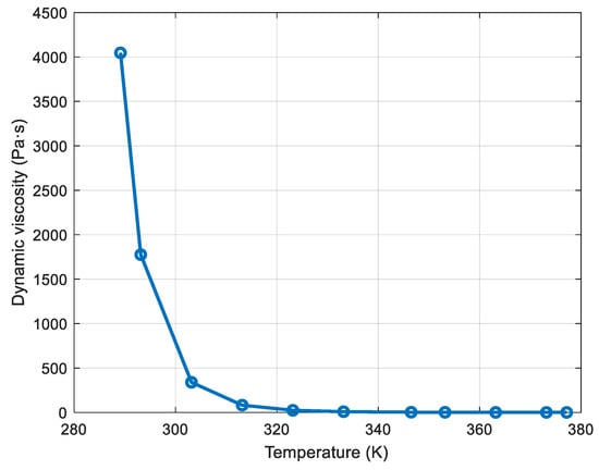
Figure 2.
Heavy crude oil viscosity API 11.2.
In CFD simulations, meshing plays a crucial role in determining the accuracy, convergence, and computational efficiency of the results. A well-designed mesh captures the critical details of the flow, such as temperatures and pressure gradients, thus ensuring the accuracy of the results [20,21]. For the meshing in this simulation, tetrahedral elements were used, as shown in Figure 3. The models employed in the mesh generation are: Edge Sizing, Volume Sizing, Face Meshing, and Smoothing (Medium).
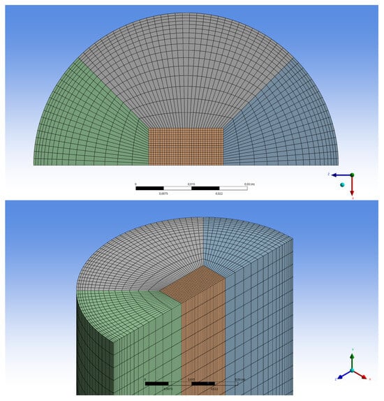
Figure 3.
Meshed model.
The minimum cell size in the radial direction is 0.001 m, while in the axial direction it is 0.005 m, to adequately capture the effects associated with the development of the thermal and velocity boundary layers. An inflation strategy was applied with a growth rate of 1.1, meaning that each successive layer increases its thickness by 10% relative to the previous one. A total of 10 inflation layers were generated, starting with the first layer adjacent to the wall at 0.001 m thick.
Radial meshing is critical to properly capturing the development of the boundary layer. Since heavy crude has high viscosity, the thermal and velocity boundary layers could be relatively thick. A higher node density was used near the wall, where the boundary layer forms. The meshing in the flow direction is uniform throughout all sections. The mesh quality was evaluated using the Skewness metric, which is recommended for CFD simulations; it measures the distortion of the cells by evaluating the difference between the actual shape of the cell and the ideal cell. The ideal value is 0, indicating a well-shaped cell, while a value close to one indicates that the mesh is deformed [22]. A total of 1,633,000 elements were used in the simulation, and Figure 3 shows the meshing applied in the simulation.
Figure 4 shows the variation in the fluid outlet temperature as a function of the mesh size used in the CFD simulation. It can be observed that as the number of elements increases, the outlet temperature converges toward a stable value. From approximately 1.6 million cells onward, the temperature variation is less than 1%, indicating that the model reaches mesh independence. Therefore, this mesh size was selected as the optimum to ensure a balance between numerical accuracy and computational cost.
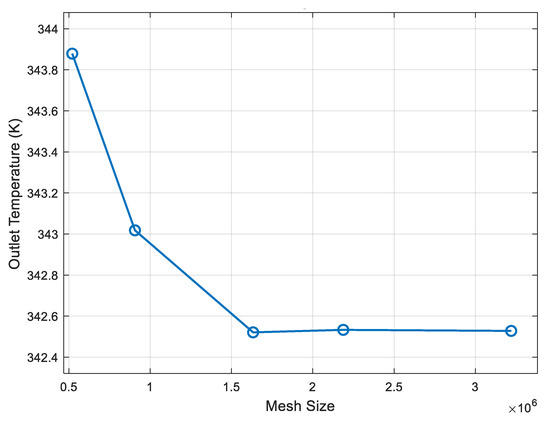
Figure 4.
Mesh independence.
2.2. Physical Models Specification
For the CFD simulation of heavy crude oil through the pipeline, with heat loss to the surroundings, several fundamental equations of fluid mechanics and heat transfer are involved. the equations governing this process are: the Navier–Stokes equations (Conservation of momentum) (1). These equations govern the behavior of fluid flow and are a specific form of the conservation laws of momentum in viscous fluids [23].
where is the density of the heavy crude oil, V is the velocity field of the fluid, p is the pressure, t is the time, and µ is the dynamic viscosity of the heavy crude oil.
Since heavy crude oil can be considered incompressible in most applications, the continuity Equation (2) is used to ensure that the fluid mass is conserved throughout the simulation domain [24,25].
This equation ensures that the amount of fluid entering any control volume is equal to the amount of fluid leaving that volume, which is important for correctly modeling the flow in the pipeline.
The energy conservation Equation (3), since heavy crude oil loses heat to the surroundings, is crucial for modeling thermal transport within the fluid and toward the pipeline walls [26].
where is the specific heat of the heavy crude oil at constant pressure, T is the temperature of the heavy crude oil, k is the thermal conductivity of the heavy crude oil, and represents the heat sources or sinks.
This equation describes the change in temperature within the crude flow due to advection (fluid motion) and heat diffusion, and how the heavy crude transfers heat to the pipeline walls and, eventually, to the external environment. To properly model the heat loss of heavy crude oil to the surroundings, it is necessary to apply heat transfer boundary conditions on the outer surface of the pipeline, these conditions are based on Newton’s law of cooling (4):
where q is the heat flux, h is the convective heat transfer coefficient on the outer surface of the pipeline, is the temperature at the inner surface of the pipeline, and is the external ambient temperature.
The flow of heavy crude oil through the pipeline is considered laminar since the Reynolds number is less than 2000, and the equation used is (5).
where V is the velocity and D is the pipeline diameter.
Another dimensionless number useful in this study is the Prandtl number, which relates the diffusion of momentum to the diffusion of heat in a fluid. In the case of heavy crude oil, this number can reach high values due to its high viscosity and low thermal conductivity. The equation used for its calculation is (6).
The exposure of the pipeline to the environment generates a significant heat exchange between the heavy crude inside and the external surroundings, making it imperative to determine the convective heat transfer coefficient. This coefficient is fundamental for understanding the efficiency of heat transport from the crude to the pipeline surface and, ultimately, to the environment. to quantify this convection process, the Nusselt number is used, a dimensionless quantity that describes the relationship between heat transfer by convection and heat transfer by conduction in the fluid’s thermal boundary layer. The Nusselt number allows for the evaluation of convection intensity and becomes a key parameter for the thermal characterization of the system. for the calculation of the Nusselt number, the Sieder and Tate correlation is used, as shown in Equation (7) [27].
where D is the pipeline diameter and L is the pipeline length.
The friction coefficient is another important dimensionless parameter in fluid mechanics, as it quantifies the resistance the fluid exerts to motion due to friction with the pipeline walls. In laminar flow, this coefficient is calculated using Equation (8).
The thermal boundary layer in a circular pipe is the region near the pipe wall where a significant temperature gradient occurs between the fluid and the pipe wall, which is why its study is important. In this region, the effects of heat conduction are more prominent than those of convection [28].
For the simulation, the SIMPLE algorithm is used because the analysis is in steady state, the flow is relatively stable, and the regime is laminar [29]. Since the heavy crude oil flow inside the pipeline involves heat transfer to the outside, the recommended spatial discretization is Second Order Upwind [30].
To facilitate the simulation of surface pumping of heavy crude oil and ensure that the model is computationally feasible, the following fundamental assumptions were made.
Steady State: The study focuses on constant operating conditions, assuming that there are no significant temporal variations in the crude oil flow [29].
Incompressible Flow: Heavy crude oil is considered an incompressible fluid, which is appropriate given that density variations are minimal and do not significantly affect the simulation results under the expected operating conditions.
Temperature-Dependent Properties: The physical properties of heavy crude oil, such as density and especially viscosity, are considered variable as a function of temperature. Since the viscosity of heavy crude changes significantly with temperature, its proper modeling is crucial to accurately reflect flow behavior. As the crude cools during transport, its viscosity increases, which affects flow dynamics and requires greater pumping power. Therefore, the simulation includes the variation in these properties throughout the domain, using appropriate rheological relationships to capture these thermal effects. To determine the dynamic viscosity as a function of temperature, Equation (9) is used [31].
where T is the crude oil temperature, and A and B are empirical constants that depend on the type of crude oil; for this case, we have that A = 8.385 × 10⁻¹⁵ y, B = 11,634.50.
For the simulation, the SIMPLE algorithm is used because the analysis is in steady state, the flow is relatively stable, and the regime is laminar [32], since the heavy crude oil flow inside the pipeline involves heat transfer to the outside, the recommended spatial discretization is Second Order Upwind [33].
To facilitate the simulation of surface pumping of heavy crude oil and ensure that the model is computationally feasible, the following fundamental assumptions were made. Steady State: The study focuses on constant operating conditions, assuming that there are no significant temporal variations in the crude oil flow [29].
Incompressible Flow: Heavy crude oil is considered an incompressible fluid, which is appropriate since density variations are minimal and do not significantly affect the simulation results under the expected operating conditions.
Temperature-Dependent Properties: The physical properties of heavy crude oil, such as density and especially viscosity, are considered variable as a function of temperature. Because the viscosity of heavy crude changes significantly with temperature, proper modeling is crucial to accurately reflect flow behavior. As the crude cools during transport, its viscosity increases, affecting flow dynamics and requiring greater pumping power. Therefore, the simulation includes the variation in these properties throughout the domain, using appropriate rheological relationships to capture these thermal effects.
Smooth Pipe Walls: To reduce the complexity of the model, the internal surfaces of the pipeline are assumed to be completely smooth. This eliminates the need to model the effects of surface roughness.
For the simulation of heavy crude oil flow under specific conditions, the following boundary conditions were defined, based on real data and operating parameters:
Fluid Velocity: 0.15758 m/s, this value was calculated based on a well production of 480 barrels per day and a pipeline inner diameter of 0.0848 m.
Fluid Temperature: 346.483 K this initial temperature was recorded in the field, reflecting the thermal conditions of the fluid as it enters the pumping system.
Atmospheric Pressure: It is assumed that the fluid outlet is exposed to atmospheric pressure. This assumption is practical to simplify the simulation, focusing on the evaluation of the fluid temperature at the end of the process.
Ambient Temperature: 292.15 K the external temperature of the pipeline is considered constant and represents the typical environmental conditions of the operating area.
These boundary conditions are designed to effectively model the behavior of heavy crude oil under a set of realistic operating assumptions, enabling an accurate simulation of the thermal and flow phenomena within the system.
2.3. Discretization of the Governing Equations
In the discretization of the governing equations for the CFD simulation in Ansys Fluent, the continuous partial differential equations are transformed into discrete algebraic equations by dividing the domain into a finite element mesh. Then, a discretization method finite volume in this case was applied to approximate the terms of the equations with suitable numerical schemes. These discretized equations were organized into a system of equations that is solved iteratively, controlling stability and convergence through adjustments in convergence criteria and relaxation factors, ensuring an accurate and stable solution of the fluid behavior [34].
2.4. Validation
The validation of the numerical model in this research was a critical step to ensure that the CFD simulation could accurately represent the behavior of the real system. This process involved a direct comparison of the results obtained through simulation with the experimental data collected, allowing for the evaluation of the model’s fidelity. The outlet temperature of the heavy crude oil was used as the reference variable, with an experimental value of 343.706 K recorded, while the simulation produced a result of 342.521 K. The minimal difference between both results translates into an absolute mean percentage error of only 0.345%, which is well below the 2% threshold considered acceptable for an accurate simulation [35,36].
3. Results
In Figure 5, the residuals are presented, which play a fundamental role in evaluating the convergence of numerical simulations. The residuals represent the difference between the values calculated by the model and the expected values of the flow variables, such as temperature, velocity, and pressure. Monitoring the residuals makes it possible to determine whether the simulation is stabilizing correctly or if significant discrepancies still exist that could indicate the need to adjust the model or improve mesh accuracy. In this study, an absolute convergence criterion of 1 × 10⁻⁹ was established [37], which implies that the differences between the simulated results and the reference values must be extremely small for the simulation to be considered to have reached a stable and accurate solution.
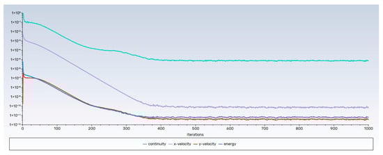
Figure 5.
Residual curves of the simulation.
In Figure 6, the temperature at the pipeline inlet can be observed, which is where the temperature is at its maximum for this simulation. The crude oil temperature at the inlet of the analyzed surface section is 346.483 K.
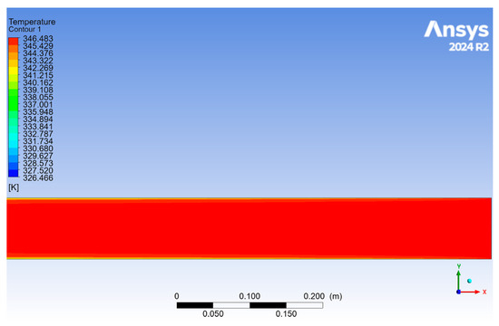
Figure 6.
Temperature at the pipeline inlet.
In Figure 7, the temperature at the pipeline outlet can be observed, which is where the temperature would be at its minimum for this simulation. The heavy crude oil temperature at the outlet of the analyzed surface section is 342.521 K.
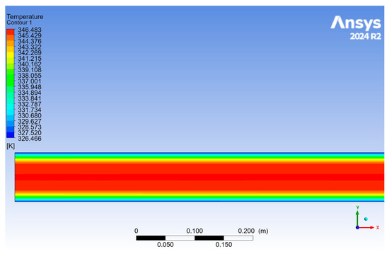
Figure 7.
Temperature at the pipeline outlet.
In Figure 8, the velocity profiles of heavy crude oil are shown at different axial positions (0, 10, 20, 30, 40, and 50 m) along a pipeline. It can be observed that as the fluid advances from 0 to 50 m, the profiles change, shifting from a wider and more distributed shape to a narrower and more centered one. This behavior is directly related to the temperature loss of the crude along the path, which causes a progressive increase in viscosity. An increase in viscosity generates greater resistance to flow, reducing velocity near the walls and concentrating the flow in the center of the conduit.
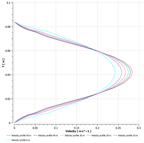
Figure 8.
Velocity profiles.
The temperature profiles shown in Figure 9 indicate that, along the pipeline, the fluid loses heat, which is reflected in a decrease in temperature near the walls, while the core maintains a higher temperature. This behavior is typical of a system where heat transfer occurs both toward the walls and to the external environment.
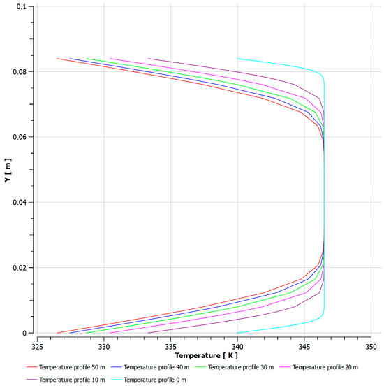
Figure 9.
Temperature profiles.
In Figure 10, the relationship between the thermal boundary layer thickness and the pipeline length transporting the heavy crude oil, which is losing heat to the environment, can be observed. A second-degree polynomial fit is shown along with the coefficient of determination.
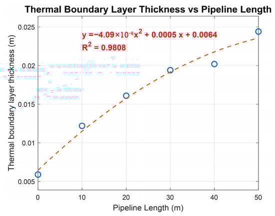
Figure 10.
Thermal boundary layer as a function of pipeline length.
The thickness of the thermal boundary layer increases along the pipeline. This behavior is typical since the fluid loses heat to the environment as it flows through the pipe. At the beginning, the thermal boundary layer is relatively small, 0.0059 m, allowing for greater heat exchange. As the crude advances through the pipeline, the thermal boundary layer grows, reaching approximately 0.0244 m at the end of the section.
In Figure 11, the variation in heavy crude oil temperatures along the 50 m pipeline can be observed. A progressive cooling is evident as the crude advances, a behavior typical of systems with heat loss to the environment, where the initial thermal gradient is greater and decreases as the crude temperature drops. The second-degree polynomial fit presents a coefficient of determination R2 = 0.9982, indicating a strong correlation between the model and the obtained data. This model is useful for estimating crude temperature in longer pipelines or segments.
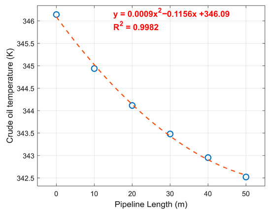
Figure 11.
Crude oil temperature as a function of pipeline length.
In Table 2, the calculated values of the Reynolds number, Prandtl number, Nusselt number, and friction coefficient are presented in 10 m intervals along the 50 m pipeline under study. It can be observed that the crude temperature decreases slightly from 346.142 K to 342.521 K, reflecting a progressive heat loss to the environment. This cooling has a direct effect on crude viscosity, increasing its value, which in turn produces a continuous decrease in the Reynolds number, from 4.851 to 4.222. Since these values are well below 2300, it confirms that the flow remains laminar along the entire section.
Table 2.
Calculation of dimensionless numbers in the pipeline section under study.
The Prandtl number increases from 43,457 to 49,952 as the crude temperature decreases. This increase is due to the rise in the crude’s dynamic viscosity at lower temperatures. Since the Prandtl number represents the ratio between momentum diffusion and heat diffusion, a higher value indicates that the fluid diffuses heat more slowly than momentum, resulting in a thinner thermal boundary layer compared to the velocity boundary layer.
Despite these changes in Reynolds and Prandtl numbers, the Nusselt number remains practically constant, suggesting that the heat transfer regime is fully developed, with conduction dominating over convection. Finally, the friction coefficient progressively increases from 13.19 to 15.16, indicating that the flow requires greater pumping effort as it advances, due to the increase in viscosity caused by thermal loss.
In Table 3, the variation in the Reynolds number, Prandtl number, Nusselt number, and friction coefficient is shown over a range of crude oil temperatures, from 289.15 K to 377.15 K, which is the operating range for its transportation.
Table 3.
Analysis of the dimensionless numbers within the crude oil temperature range.
This analysis shows that the Reynolds number increases exponentially with temperature, from 0.003 to 42.236. This is due to the drastic reduction in dynamic viscosity as the crude oil heats up. Throughout the entire working range, the flow remains laminar (Re < 2300), with easier transport at higher temperatures. The Prandtl number decreases from very high values (>67 million) to values close to 4888. This behavior is characteristic of highly viscous fluids with low thermal conductivity, such as heavy crude oil. At low temperatures, the thermal boundary layer is very thin compared to the velocity boundary layer, which hinders heat transfer. The Nusselt number remains practically constant throughout the range, confirming that heat transfer in this regime is governed by conduction and that the flow is thermally developed even with abrupt changes in viscosity. The friction coefficient decreases from 19,716 to 1.51 as the temperature increases. This decline confirms that the pumping effort required under cold conditions is very high, which can pose a serious problem for pump operation if the crude oil is not kept warm.
The results obtained, both from experimental measurements and from the CFD simulation, show a decrease in crude oil temperature from 346.483 K at the inlet point to 342.521 K at the end of a 50 m pipeline section. This temperature reduction is due to thermal interaction with the environment, whose temperature is 292.15 K, with convection being the main mechanism of heat loss. The convective coefficient determined through the simulation is 5 W/m2·K, which provides a quantitative measure of the heat transfer from the crude oil to the surroundings. This coefficient value is crucial for the analysis of longer pipeline sections, as it allows for more accurate calculation of the amount of heat lost during transport and, therefore, the amount of thermal energy that must be added to keep the crude viscosity at optimal operating levels. The temperature loss not only increases crude viscosity, making its flow more difficult, but also raises the energy requirements for pumping, affecting transport efficiency and increasing operating costs.
The fact that the velocity boundary layer is relatively large compared to the pipeline diameter (0.038 m boundary layer versus 0.084 m diameter) is due to several factors related to the properties of heavy crude oil and the flow conditions, which are detailed below:
High viscosity of heavy crude oil: due to the high viscosity of heavy crude oil (2.4606 kg/m·s), the velocity boundary layer is thick, because viscosity resists flow and delays the development of higher velocities as one move away from the pipe wall. In heavy crude, momentum transfer occurs more slowly, leading to a smoother transition from zero velocity at the wall to the main flow velocity.
Laminar flow: due to the low flow velocity of the crude (0.15758 m/s) and its high viscosity (2.4606 kg/m·s), the flow in the pipeline is laminar instead of turbulent. As a result, the boundary layer tends to be thicker. In laminar flows, the fluid moves in parallel layers and mixing between them is minimal. This means that the fluid near the pipe wall moves more slowly, and the boundary layer grows more.
Low flow velocity: the flow velocity is low (0.15758 m/s), which favors a slower development of velocity across the pipe radius. Because of the low speed, the boundary layer tends to expand since viscous forces dominate over inertial forces, delaying the establishment of a high-velocity flow.
Relationship between diameter and fluid characteristics: in pipelines of relatively small diameter, such as 0.084 m, with heavy crude oil, the boundary layer can occupy a significant portion of the velocity profile. This occurs because the space available for the flow to reach its maximum velocity is limited.
The thermal boundary layer has a particular behavior. In the first meters of the pipeline, the fluid transfers a significant amount of heat to the environment, causing a rapid increase in the thermal boundary layer. This is reflected in the almost linear behavior of Figure 8 up to the first 30 m. After 30 m, the growth of the thermal boundary layer slows down, suggesting that the fluid has lost much of its heat and the rate of heat transfer to the environment has decreased. This is typical behavior in flows with significant heat loss: as the fluid cools, the temperature gradient between the fluid and the environment decreases, reducing the rate of heat transfer. The negative quadratic term obtained in the second-degree polynomial suggests that the growth of the thermal boundary layer slows down with distance, which coincides with the trend observed in heat exchange systems where as the fluid cools, heat transfer becomes less efficient.
The velocity and thermal boundary layers are similar in behavior, but they depend on different factors. The velocity boundary layer depends on the viscosity and inertia of the fluid, while the thermal boundary layer is more related to the thermal properties of the fluid, such as thermal conductivity and heat diffusion.
In this case, the velocity boundary layer is 0.038 m in a pipeline of 0.084 m diameter. The thermal boundary layer starts at small values (around 0.0071 m) and gradually increases along the pipeline, reaching a maximum value of 0.0291 m at 50 m. This suggests that heat transfer is occurring more gradually along the pipeline, while the velocity boundary layer establishes more quickly.
4. Discussion
The results obtained in this study demonstrate that the surface transportation of heavy crude oil cannot be analyzed solely from a conventional thermodynamic perspective, as its physical properties—particularly viscosity and thermal diffusivity—are strongly temperature-dependent, generating a nonlinear flow behavior along the pipeline. Table 3 reveals that as temperature decreases, the Reynolds number abruptly drops to values close to zero (Re ≈ 0.003), while the Prandtl number exceeds 107. This regime represents a transition toward quasi-static or gel-like flow conditions, in which classical hydraulic correlations (such as the Hagen–Poiseuille friction factor) lose validity, as they assume a Newtonian fluid with continuous deformation and stable flow characteristics. Under these conditions, flow resistance is governed by the viscoelastic behavior of the crude and the micro-structuring of heavy molecules, highlighting the need for future studies to incorporate non-Newtonian rheological models such as Bingham or Herschel–Bulkley.
Additionally, boundary layer analysis confirms that the flow is hydrodynamically developed, but thermally developing due to the high Prandtl numbers. As quantitatively demonstrated, a δt/δv ≈ Pr−1/3 relationship for Pr values in the range of 103–105 implies that the thermal boundary layer may be 10 to 40 times thinner than the velocity boundary layer, restricting heat transfer to only a minimal fraction of the pipe cross-section. This condition physically explains why, despite moderate Nusselt numbers, the film coefficient h remains low due to the limited thermal diffusivity and low thermal conductivity of the crude oil.
Regarding the polynomial model used to represent temperature loss, although the R2 values are high (close to 0.998), it is important to recognize that this is an empirical fit within a specific thermodynamic domain; therefore, extrapolation to longer pipeline lengths must be approached with caution. The negative quadratic term indicates a progressive decrease in the heat loss rate as the fluid cools, which is physically consistent with the thickening of the thermal boundary layer. However, extrapolation beyond the validated domain could underestimate the critical point at which the crude transitions into a non-Newtonian or flow-discontinuity regime. Thus, the model is limited to fluids within the studied temperature range and to conditions in which the Reynolds number remains above the operational threshold for pumpable flow.
Finally, the results of this study should be interpreted as a predictive tool for thermal optimization rather than as a universal model for all transportation conditions. Identifying a critical temperature and distance beyond which the crude loses its pumpability has significant operational implications, as it enables the design of targeted insulation or intermediate heating strategies to prevent hydraulic collapse of the flow. This discussion synthesizes the findings and provides a robust conceptual framework that supports decision-making in the design and operation of heavy crude oil pipelines.
5. Conclusions and Recommendations
This study developed and validated a computational fluid dynamics model with temperature-dependent properties to analyze the thermo-hydraulic behavior of heavy crude oil along a 50 m SCH-80 pipeline segment under real operating conditions in the Ecuadorian Oriente. The results show a temperature decrease from 346.5 K to 342.5 K, which led to a significant increase in viscosity and a reduction in the Reynolds number to values on the order of 5, demonstrating the direct impact of thermal loss on flow behavior. It was also determined that the thermal boundary layer reached only 13% of the pipe radius, while the velocity boundary layer extended up to 60%, confirming that heat transfer is limited by the low thermal diffusivity of the crude. Moreover, an effective external convective heat transfer coefficient of 5 W·m−2·K was obtained, and a second-degree polynomial model with a determination coefficient (R2) of 0.998 was developed, enabling highly accurate prediction of temperature loss along the pipeline and providing a valuable tool for the design of longer transportation systems.
The analysis of dimensionless numbers revealed that decreasing temperature leads to an exponential increase in the Prandtl number (exceeding 107) and a drop in the Reynolds number to values close to zero, indicating quasi-static flow conditions and potential gelation. This behavior demonstrates that even minor heat losses can trigger hydraulic flow failure, making thermal maintenance of the fluid a critical operational requirement. In this context, the proposed model not only identifies the sections where temperature loss is most pronounced, but also provides a scientific basis for defining insulation and heating strategies that ensure operational continuity, reduce pumping costs, and prevent blockages associated with crude oil cooling.
In summary, the findings of this study provide unprecedented quantitative evidence of the interaction between thermal and dynamic phenomena in the surface transportation of heavy crude oil and lay the foundation for the development of advanced thermal management technologies. Future research may extend this model by incorporating non-Newtonian rheological behavior and experimental validation over longer distances, with the aim of developing applied solutions that enhance energy efficiency and promote the sustainability of crude oil transportation in the petroleum industry.
Author Contributions
Conceptualization, E.B.-P. and C.D.R.-G.; Methodology, J.C.-E.; Software, J.C.-E.; Investigation, P.V.C.; Writing—review and editing, L.C.-V. and D.B. All authors have read and agreed to the published version of the manuscript.
Funding
This study received no external funding.
Data Availability Statement
The original contributions presented in this study are included in the article. Further inquiries can be directed to the corresponding author.
Acknowledgments
The authors thank the Dirección de Investigación y Desarrollo (DIDE) of the Universidad Técnica de Ambato for supporting this work through the research project PFICM38, “Evaluación y optimización de un sistema híbrido de generación eléctrica mediante aerogeneradores de eje vertical (VAWT) mediante Dinámica de Fluidos Computacional (CFD) y paneles solares fotovoltaicos mediante el software PVSOL para comunidades rurales de la sierra ecuatoriana sin acceso a energía eléctrica”.
Conflicts of Interest
The authors declare no conflicts of interest.
References
- Souas, F.; Safri, A.; Benmounah, A. A review on the rheology of heavy crude oil for pipeline transportation. Pet. Res. 2021, 6, 116–136. [Google Scholar] [CrossRef]
- Speight, J.G. Chapter 1-occurrence and formation of crude oil and natural gas. In Subsea and Deepwater Oil and Gas Science and Technology; Elsevier: Amsterdam, The Netherlands, 2015; pp. 1–43. [Google Scholar]
- Alboudwarej, H.; Felix, J.; Taylor, S.; Badry, R.; Bremner, C.; Brough, B.; Skeates, C.; Baker, A.; Palmer, D.; Pattison, K.; et al. La importancia del petróleo pesado. Oilfield Rev. 2006, 18, 38–58. [Google Scholar]
- Zou, C. Heavy oil and bitumen. In Unconventional Petroleum Geology; Elsevier: Amsterdam, The Netherlands, 2017; pp. 345–370. [Google Scholar]
- Meriem-Benziane, M.; Abdul-Wahab, S.A.; Benaicha, M.; Belhadri, M. Investigating the rheological properties of light crude oil and the characteristics of its emulsions in order to improve pipeline flow. Fuel 2012, 95, 97–107. [Google Scholar] [CrossRef]
- Ramírez, J.; Zambrano, A.; Ratkovich, N. Prediction of Temperature and Viscosity Profiles in Heavy-Oil Producer Wells Implementing a Downhole Induction Heater. Processes 2023, 11, 631. [Google Scholar] [CrossRef]
- Kumar, P.; Singh, J. Computational study on effect of Mahua natural surfactant on the flow properties of heavy crude oil in a 90° bend. Mater. Today Proc. 2021, 43, 682–688. [Google Scholar] [CrossRef]
- Zhong, H.; Shi, B.; Bi, Y.; Cao, X.; Zhang, H.; Yu, C.; Tang, H. Interaction of elasticity and wettability on enhanced oil recovery in viscoelastic polymer flooding: A case study on oil droplet. Geoenergy Sci. Eng. 2025, 250, 213827. [Google Scholar] [CrossRef]
- Li, H.; Zhang, J. Viscosity prediction of non-Newtonian waxy crude heated at various temperatures. Pet. Sci. Technol. 2014, 32, 521–526. [Google Scholar] [CrossRef]
- Cazorla, J.J. Evaluación de la Producción y el Factor de Recobro en Yacimientos de Crudo Extra Pesado a Través de la Aplicación de Ondas Electromagnéticas en Pozos Horizontales. 2013. Available online: http://saber.ucv.ve/handle/10872/4261 (accessed on 18 February 2024).
- Tolentino, S.L.; Caraballo, S.; Duarte, Á.; Mendoza, J. Calentamiento de yacimientos petrolíferos mediante cápsulas de reacción nuclear. Univ. Cienc. Tecnol. 2016, 20, 58–68. Available online: http://ve.scielo.org/scielo.php?script=sci_arttext&pid=S1316-48212016000200001&lng=es&nrm=iso&tlng=es (accessed on 18 February 2024).
- Saleh, S.N.; Mohammed, T.J.; Hassan, H.K.; Barghi, S. CFD investigation on characteristics of heavy crude oil flow through a horizontal pipe. Egypt. J. Pet. 2021, 30, 13–19. [Google Scholar] [CrossRef]
- Zhang, L.; Du, C.; Wang, H.; Zhao, J. Three-dimensional numerical simulation of heat transfer and flow of waxy crude oil in inclined pipe. Case Stud. Therm. Eng. 2022, 37, 102237. [Google Scholar] [CrossRef]
- R, R.K.; Karthik, K.; Elumalai, P.; Alshahrani, S.; Ağbulut, Ü.; Saleel, C.A.; Shaik, S.; Khan, S.A. Investigation of nano composite heat exchanger annular pipeline flow using CFD analysis for crude oil and water characteristics. Case Stud. Therm. Eng. 2023, 49, 103297. [Google Scholar] [CrossRef]
- Cabrera Escobar, J.; Sotomayor, G.M.; Carrazco, D.C.; Godoy, M.M.P.; Cabrera-Escobar, R. CFD simulation of the surface pumping of heavy crude oil in eastern Ecuador. Enfoque UTE 2024, 15, 35–40. [Google Scholar] [CrossRef]
- Meriem-Benziane, M.; Bou-Saïd, B.; Abdelkader, B. A CFD modeling of oil-water flow in pipeline: Interaction analysis and identification of boundary separation. Pet. Res. 2021, 6, 172–177. [Google Scholar] [CrossRef]
- Tu, Q.; Ma, Z.; Wang, H. Investigation of wet particle drying process in a fluidized bed dryer by CFD simulation and experimental measurement. Chem. Eng. J. 2023, 452, 139200. [Google Scholar] [CrossRef]
- Getahun, E.; Delele, M.A.; Gabbiye, N.; Fanta, S.W.; Demissie, P.; Vanierschot, M. Importance of integrated CFD and product quality modeling of solar dryers for fruits and vegetables: A review. Sol. Energy 2021, 220, 88–110. [Google Scholar] [CrossRef]
- Tegenaw, P.D.; Gebrehiwot, M.G.; Vanierschot, M. On the comparison between computational fluid dynamics (CFD) and lumped capacitance modeling for the simulation of transient heat transfer in solar dryers. Sol. Energy 2019, 184, 417–425. [Google Scholar] [CrossRef]
- Umuteme, O.M.; Islam, S.Z.; Hossain, M.; Karnik, A. An improved computational fluid dynamics (CFD) model for predicting hydrate deposition rate and wall shear stress in offshore gas-dominated pipeline. J. Nat. Gas Sci. Eng. 2022, 107, 104800. [Google Scholar] [CrossRef]
- Haghshenasfard, M.; Hooman, K. CFD modeling of asphaltene deposition rate from crude oil. J. Pet. Sci. Eng. 2015, 128, 24–32. [Google Scholar] [CrossRef]
- ANSYS Inc. ANSYS Meshing User’s Guide; ANSYS Inc.: Canonsburg, PA, USA, 2024; Available online: https://ansyshelp.ansys.com/account/secured?returnurl=/Views/Secured/corp/v242/en/wb2_help/wb2_help.html (accessed on 15 August 2025).
- Xiao, Y.; Cai, Y.; Sun, C.; Cui, G.; Xu, Z.; Wang, P.; Jia, L. Bionic pipeline transport characteristics with transverse protuberances in slurry shield circulation system based on CFD-DEM. Powder Technol. 2024, 432, 119133. [Google Scholar] [CrossRef]
- Garg, K.; Singh, S.; Rokade, M.; Singh, S. Experimental and computational fluid dynamic (CFD) simulation of leak shapes and sizes for gas pipeline. J. Loss Prev. Process Ind. 2023, 84, 105112. [Google Scholar] [CrossRef]
- Zhao, J.; Zhao, W.; Chi, S.; Zhu, Y.; Dong, H. Quantitative effects of different factors on the thermal characteristics of waxy crude oil pipeline during its shutdown. Case Stud. Therm. Eng. 2020, 19, 100615. [Google Scholar] [CrossRef]
- Cheng, Q.; Gan, Y.; Wang, P.; Sun, W.; Xu, Y.; Liu, Y. The study on temperature field variation and phase transition law after shutdown of buried waxy crude oil pipeline. Case Stud. Therm. Eng. 2017, 10, 443–454. [Google Scholar] [CrossRef]
- Holman, J.P. Heat Transfer, 10th ed.; McGraw-Hill: New York, NY, USA, 2010. [Google Scholar]
- Zeng, G.; Chen, L.; Yang, D.; Yuan, H.; Zang, J.; Huang, Y. Measurement and comparison of transient thermal boundary layer of a Local-Heated Mini-Channel under sub- and super-critical conditions. Appl. Therm. Eng. 2024, 247, 123053. [Google Scholar] [CrossRef]
- ANSYS Inc. ANSYS Fluent Tutorial Guide, 2023 R1; ANSYS Inc.: Canonsburg, PA, USA, 2023. [Google Scholar]
- Benhamza, A.; Boubekri, A.; Atia, A.; Hadibi, T.; Arıcı, M. Drying uniformity analysis of an indirect solar dryer based on computational fluid dynamics and image processing. Sustain. Energy Technol. Assess. 2021, 47, 101466. [Google Scholar] [CrossRef]
- Cabrera-Escobar, J.; Jurado, D.V.F.; Córdova-Suárez, M.; Santillán-Valdiviezo, G.; Rodríguez-Orta, A.; Cabrera-Escobar, R. Optimization of olive pomace dehydration process through the integration of computational fluid dynamics and deep learning. Energy Sources Part A Recovery Util. Environ. Eff. 2024, 46, 4756–4776. [Google Scholar] [CrossRef]
- American Petroleum Institute. Technical Data Book—Petroleum Refining, 2nd ed.; American Petroleum Institute: Washington, DC, USA, 2013. [Google Scholar]
- ANSYS Inc. ANSYS Fluent Theory Guide, 2023 R1; ANSYS Inc.: Canonsburg, PA, USA, 2023. [Google Scholar]
- Zhao, J.; Liu, J.; Dong, H.; Zhao, W.; Wei, L. Numerical investigation on the flow and heat transfer characteristics of waxy crude oil during the tubular heating. Int. J. Heat Mass Transf. 2020, 161, 120239. [Google Scholar] [CrossRef]
- Hussain, F.; Jaskulski, M.; Piatkowski, M.; Tsotsas, E. CFD simulation of agglomeration and coalescence in spray dryer. Chem. Eng. Sci. 2022, 247, 117064. [Google Scholar] [CrossRef]
- Cabrera-Escobar, J.; Vera, D.; Jurado, F.; Cabrera-Escobar, R. CFD investigation of the behavior of a solar dryer for the dehydration of olive pomace. Energy Sources Part A Recovery Util. Environ. Eff. 2024, 46, 902–917. [Google Scholar] [CrossRef]
- Xie, H.; Li, C.; Jia, W.; Zhang, C. Three-Dimensional CFD Modeling on the Thermal Characteristics of Buried Oil Pipeline Involving the Heat Transfer of Wax Layer. Energies 2022, 15, 6022. [Google Scholar] [CrossRef]


Disclaimer/Publisher’s Note: The statements, opinions and data contained in all publications are solely those of the individual author(s) and contributor(s) and not of MDPI and/or the editor(s). MDPI and/or the editor(s) disclaim responsibility for any injury to people or property resulting from any ideas, methods, instructions or products referred to in the content. |
© 2025 by the authors. Licensee MDPI, Basel, Switzerland. This article is an open access article distributed under the terms and conditions of the Creative Commons Attribution (CC BY) license (https://creativecommons.org/licenses/by/4.0/).