Abstract
Centralized heating systems in severe cold regions suffer from widespread load estimation deviations due to architectural heterogeneity and a lack of construction drawings, leading to substantial energy waste. This study proposes a lightweight load calculation method that facilitates efficient calculation of heating loads for heterogeneous building clusters via spatial thermal pattern decoupling and matrix reorganization. First, a 3 × 3 load characteristic matrix is developed to characterize the spatial variation in thermal demand across different building positions (corner vs. intermediate units × top, middle, and bottom floors), revealing that corner units exhibit higher thermal loads than intermediate units, while top and bottom floors show significantly higher loads than middle floors. Second, two complementary matrices are established: the load characteristic matrix, which represents the building’s thermal behavior, and the structural feature matrix, which encodes the architectural configuration in terms of unit count (a) and floor count (b). Together, they enable rapid hourly load synthesis using only lightweight input parameters. The method is validated on 56 heterogeneous residential buildings in Northeast China. Using a decoupled 4U/6F standard model, the synthesized cluster heating load achieves an R2 of 0.88, an RMSE of 24.15 GJ, a MAPE of 4.94%, and a Mean Percentage Error (MPE) of −0.82% against actual heating supply data, demonstrating high accuracy and negligible systematic bias—particularly during cold waves. This approach allows the seasonal variation in heat demand across an entire residential area to be estimated even in the absence of detailed construction drawings, offering practical guidance for operational heating management.
1. Introduction
According to the 2024 International Energy Agency (IEA) report World Energy Balance [1], building energy consumption accounts for approximately 30% of global total energy use and 40% of global carbon emissions. Data from a 2024 research report on China’s urban-rural development [2] indicates that building operational processes constitute 22% of the national total energy consumption (about 1.19 billion tce), with centralized heating systems consuming 170 million tce. Heating supply per unit area decreased from 0.98 GJ/m2 in 2000 to 0.38 GJ/m2 in 2022 (a 61.7% reduction), demonstrating that optimizing energy supply structures significantly reduces centralized heating energy consumption.
Jiang et al. [3] report China’s heated floor area expanded from 5.0 billion m2 in 2001 to 15.6 billion m2 in 2020. District heating systems dominate in northern cities, comprising heat sources, heat exchange stations, and end-users [4]. Heat generated from sources is transported via primary pipe networks to exchange stations, then distributed to end-users through secondary pipe networks [5]. User demand fluctuates with ambient conditions, yet operators frequently overestimate heating demand to minimize complaints [6]. Consequently, users passively accept all supplied heat, with few residents adjusting inlet valves for energy savings—most dissipate excess heat by opening windows, causing substantial energy waste due to the supply side’s inability to rapidly identify building-specific heating demand [7].
Centralized heating has evolved to the Fourth-Generation District Heating (4GDH) [8], initially proposed by Danish scholars [9], emphasizing smart energy system integration. Innovations include waste-heat recovery components [6], advanced thermal storage schemes [10], and renewable energy integration [11]. Recently, Fifth-Generation District Heating (5GDH) was proposed to enhance urban heating intelligence [12], where rapid building load prediction becomes fundamental for smart heating operation and bridges supply–demand responses [13,14].
Multiple methodologies exist for calculating building heating loads, categorized into physical models (white-box) [12], data-driven approaches (black-box) [13], and hybrid methods (grey-box models) [14]. White-box models employ physics-based equations for forward modeling [15,16], extensively utilized in building energy simulation due to their strong interpretability and formula-driven reliability in tracing heat flow paths [17]. However, they exhibit poor generalizability—models developed for specific buildings fail to extrapolate to other configurations even with identical internal layouts, primarily due to variations in unit counts and floor heights. Black-box models minimally utilize physical principles [18,19], instead relying on historical data to construct and optimize model parameters for complex prediction tasks where physical formulations prove infeasible [20]. Their physics-agnostic predictions result in low interpretability, requiring substantial high-quality datasets for viable model training. Grey-box models integrate the strengths of both approaches [21], balancing interpretability and adaptability by calibrating parameters with operational datasets [22], thereby simplifying building representations while maintaining robust real-world performance.
Grey-box models have been deployed across diverse built environments: Tugores, Macarulla, and Gangolells [23] integrated indoor aerodynamics with thermodynamics to enhance thermal comfort, demonstrating ≥ 15% energy efficiency gains with IAQ-3, IAQ-4, and T-6 models. Yu et al. [24] implemented adaptive Model Predictive Control (MPC) mechanisms to mitigate accuracy degradation in Linear Time-Invariant (LTI) grey-box models during abrupt weather shifts. Zhang et al. [25] developed a three-phase load testing methodology for underground structures, validating a sub-6% error grey-box model across nine Qingdao subway stations. Xie, Li, and Hong [26] created physics-embedded neural networks via meta-learning, achieving climate adaptability while balancing interpretability and computational efficiency. Lin et al. [27] leveraged RC models to quantify unmeasured internal heat gains from envelope upgrades by comparing computed and monitored temperatures, overcoming limitations of pure data-driven approaches. Serasinghe, Long, and Clark [28] optimized RC model parameter initialization—identified as the most critical challenge—by classifying models and seeding analogous initial parameters to ensure computational efficiency.
Recent advances in reduced-order modeling and machine learning have opened new pathways for efficient and accurate prediction of building heating loads, particularly in the context of district heating systems operating in cold climates. A growing body of literature explores hybrid strategies that combine physical principles with data-driven techniques to balance computational efficiency, model fidelity, and scalability. Representative studies include the following:
Jiang et al. [29] developed a method for predicting fluid temperature dynamics in district heating pipeline networks to estimate building thermal loads. The team established a simplified relationship among pipe outlet temperature, inlet temperature, and ground temperature by applying energy conservation principles to each pipe segment. Training data were generated either from physics-based “full-order models” (FOMs) or from experimental measurements. The authors demonstrated that, compared to conventional approaches, their method achieves a computational cost reduction in several orders of magnitude—particularly in networks with complex pipeline configurations.
Silvestri et al. [30] leveraged architectural drawings from the building design phase to construct a white-box model using TRNSYS. Based on the outputs of this physics-based model, they subsequently developed a grey-box model of the building. In this process, two key thermal parameters were identified and estimated using three distinct grey-box modeling approaches. Their analysis showed that the resulting simplified models retain high prediction accuracy despite a significant reduction in model complexity.
Abdel-Jaber and Dirks [31] provided a comprehensive review of data-driven approaches for predicting building heating and cooling loads. The survey covers a wide range of machine learning techniques—including ensemble learning, support vector machines (SVMs), artificial neural networks (ANNs), statistical models, and probabilistic models—and further compares commonly used datasets, modeling platforms, and the interpretability of these predictive models.
Zhang et al. [32] observed that occupant behavior and building envelope characteristics exhibit substantial uncertainty across different buildings. To address this, they proposed an integrated framework that combines physics-based energy simulation, machine learning, and multi-objective optimization to quantify such uncertainties. Specifically, they employed XGBoost as a surrogate for detailed building energy models, achieving an 89.7% reduction in computational time. When validated on a single-family residential building in Canada, the surrogate model achieved an R2 of 0.85 in predicting energy consumption.
Weber et al. [33] introduced a machine learning-based framework to estimate the impact of energy retrofit measures—such as roof and wall insulation upgrades and window replacements—on building energy use. By integrating machine learning with causal inference, they quantified the effectiveness of various retrofit strategies. The study also highlighted a critical challenge: the scarcity of large-scale, high-quality building load datasets, which currently limits the potential for deeper model optimization and generalization.
This paper addresses key challenges in reduced-order modeling (ROM) and machine learning-enhanced heating load prediction for buildings in cold climates, and proposes a computationally efficient methodology for estimating community-scale building thermal loads.
This study aims to develop a lightweight, scalable method for estimating heating loads in heterogeneous residential clusters—particularly those lacking architectural drawings—by decoupling spatial thermal patterns and reorganizing structural information into interpretable matrices.
The article is structured as follows:
Section 2 details geographical context (43.88° N, 126.57° E), heating-season weather patterns, and building structural modeling with load calculation methodology.
Section 3 applies spatial pattern decoupling to standard buildings, computes hourly loads for heterogeneous configurations, integrates computational results, and performs comparative analysis with operational data from the heating station.
Section 4 discusses computational advantages for future grey-box modeling implementations.
2. Methods and Model
Current grey-box research predominantly focuses on single-building or room-level load prediction [34,35,36], neglecting methodologies to scale calculated loads across heterogeneous building clusters. This study introduces a matrix-based decoupling approach to disentangle room thermal characteristics from structural specifications (unit count a and floor number b), enhancing generalizability for apartment-style buildings with identical room layouts but varying configurations—a typology prevalent in Northeast China [37]. These 1980s-era structures [38] suffer from aged pipelines and obsolete heating systems, originally designed without energy-efficiency considerations, resulting in inflexible operation and suboptimal parameterization. Their ad hoc construction nature led to incomplete architectural drawings, preventing comprehensive white-box modeling. Since 2014, China’s retrofit initiatives have prioritized upgrading such systems [39], focusing on pipe replacement and thermal load rebalancing.
The spatial pattern decoupling-based load calculation method proposed in this work fundamentally differs from conventional building load calculation approaches, such as deriving thermal loads through architectural modeling with complete parameter specifications, or obtaining load data via machine learning when substantial high-quality heating operation data exists from long-term system monitoring. This method is specifically tailored for existing or newly constructed residential clusters where smart heating systems have not yet been deployed; thus, detailed heating parameters are unavailable, while all buildings share identical internal room layouts but differ exclusively in unit count (a) and floor count (b) configurations.
We implement a three-phase methodology using Jilin City’s Qingsong Community as a case study:
First, spatial thermal pattern decoupling through room geometry measurement, DOE-2.3-based BESI software (BESI (2024 edition)) computation of hourly heating loads, and separation of room characteristics from structural features.
Second, matrix reorganization to generate hourly loads for diverse configurations by modifying structural matrices.
Third, aggregation of cluster-wide loads and validation against operational data from the heating station.
Compared to conventional grey-box models, this matrix decoupling achieves three fundamental breakthroughs: transcending from single-building modeling to heterogeneous cluster load synthesis; evolving from black-box prediction to physically interpretable spatial thermal patterns; and transitioning from parametric complexity to lightweight inputs requiring only unit count (a) and floor number (b).
2.1. Site Description and Climatic Conditions
This study selects a typical centralized heating community in Northeast China, located in Ningjiang District, Songyuan City, Jilin Province. As illustrated in Figure 1, the case community is located in a severe cold region [40] of China, characterized by a temperate continental monsoon climate with distinct seasons, which features prolonged winters and extremely low temperatures.
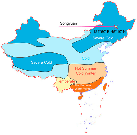
Figure 1.
Typical climate zones of China.
The winter hourly and daily outdoor temperatures in the case study area are shown in Figure 2. The minimum daily average outdoor temperature reaches −20.9 °C, while the highest temperatures occur during the initial and final phases of the heating season, exceeding 18 °C. Additionally, the diurnal temperature variation averages 10 °C, indicating a characteristically severe winter climate.
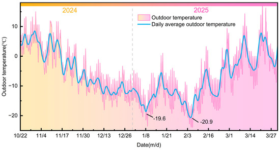
Figure 2.
Hourly outdoor temperature and daily outdoor temperature.
The distribution of apartment-style buildings requiring heating in the case study community is shown in Figure 3, with multiple architectural typologies present. In the figure, “U” (Unit) denotes the number of units per building, representing building length and ranging from 1 to 5. The color blocks representing buildings are stretched proportionally to unit count—buildings with more units exhibit wider blocks. “F” (Floor) indicates floor numbers ranging from 4 to 6, where higher floors correspond to darker color blocks. Consequently, the size and color of these blocks provide fundamental building information.
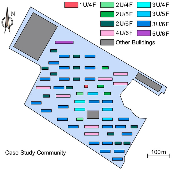
Figure 3.
Spatial distribution map of apartment-style buildings in the case study community.
The internal room layout is depicted in Figure 4. All buildings feature one staircase serving two households, with rooms symmetrically distributed. Each household comprises four rooms: living room, master bedroom, secondary bedroom, and bathroom. The master bedroom is located on the south side with south-facing windows, while the secondary bedroom faces north with north-facing windows. Regardless of building position, these two bedrooms always have windows for external heat exchange. Conversely, bathroom window presence varies depending on spatial location within the building. The living room has windows on both the north and south sides. Compared to other floors, the first floor lacks a balcony area in the living room, resulting in a household area of 80.11 m2 for the first floor and 88.45 m2 for the upper floors. A building may contain multiple units; adjacent units share connecting walls, where bathrooms lack windows. During load calculation, the staircase is assumed to have zero heating demand (0 W/m2).
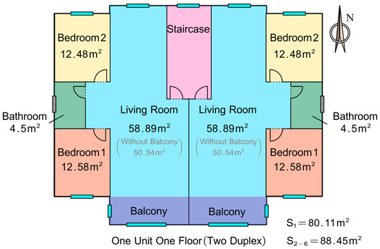
Figure 4.
Interior room layout and room areas within the building.
Detailed typologies of all apartment-style buildings in the case study community are summarized in Table 1. The community includes nine distinct architectural typologies, totaling 56 buildings with a combined area of 158,520.46 m2. All buildings share identical internal room structures as shown in Figure 4. Heating is supplied by a central heating station servicing an area of 472,600 m2, which provides daily heat supply data for the 2024–2025 heating season. All 56 buildings involved in this study feature regular structural layouts, as shown in Figure 5. Building units are arranged horizontally, rooms have windows facing north and south, and the stairwell opens toward the north.

Table 1.
Quantity and floor area of architectural typologies in the case study community.
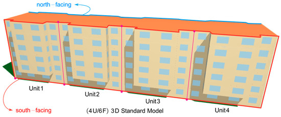
Figure 5.
Three-dimensional architectural structure of the 4U/6F standard model.
2.2. Building Thermal Load Calculation
To comprehensively cover all room scenarios in building load calculations, we select the 4U/6F architectural typology as the standard model. The load data is computed using BESI—a building energy simulation software with the DOE-2 [41] calculation engine at its core. Developed jointly by the U.S. Department of Energy (DOE) and Lawrence Berkeley National Laboratory (LBNL) in the 1970s, the DOE-2 kernel was designed to address building energy efficiency optimization needs during the energy crisis.
Within DOE-2, heat load calculations for opaque envelope assemblies (e.g., walls, roofs) utilize the response factor method. This approach characterizes dynamic heat transfer through predefined X, Y, Z response coefficients. The heat flux at the interior surface induced by exterior surface temperature perturbations is given by:
In the equation: denotes the exterior surface response coefficient, characterizing the influence of external surface temperature fluctuations on interior heat flux; represents the interior surface response coefficient, quantifying the attenuation effect of interior surface temperature on its own heat flux; describes the autocorrelation effect of historical interior surface heat flux values on the current heat flux; and denote the exterior and interior surface temperatures of the building envelope, respectively (units: K); is the default time step.
Response factors are obtained by solving the one-dimensional heat conduction equation: where denotes the thermal diffusivity, with : thermal conductivity, : density, and : specific heat capacity. For multilayer structures, the response factors of individual layers are combined through matrix multiplication.
The transmitted solar radiation load through windows is given by:
In the equation: : Shading coefficient accounting for internal and external shading devices; : Window area (m2); : Window transmittance; : Total solar radiation intensity (W/m2); : Solar radiation load factor, typically ranging 0.2–0.8 depending on the heat storage characteristics of the room.
The heat load calculation formula for solar radiation absorbed by building envelope structures is:
In the equation, is the absorptivity of the external envelope surface, is the direct solar radiation intensity (W/m2), is the solar incidence angle (radians), is the attenuation coefficient dependent on material thermal inertia, and is the time constant governing heat transfer dynamics (s−1).
Internal heat disturbances from occupants, equipment, and lighting are converted into heat loads via heat flow distribution coefficients:
In the equation, is the convective heat transfer rate of the k-th heat disturbance source (W), is the radiative heat transfer rate of the k-th source (W), and is the weighting factor characterizing the delayed release proportion of radiative heat.
2.3. Architectural Model Construction and Simulation
A 3D architectural structure of the 4U/6F standard model was constructed as shown in Figure 5, with clear differentiation between north–south orientations. The building units are sequentially labeled Unit1 to Unit4 from west to east. The solar shading effect of balconies is visually evident in the figure, which directly influences time-dependent building load variations.
Rooms in the standard model are abstracted as cubic volumes (Figure 6). The model comprises 4 units, with 2 households per unit per floor, totaling 6 floors. To uniquely identify any room, a spatial coordinate system is employed:
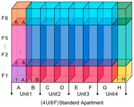
Figure 6.
Abstract structure of 4U/6F standerd architecture.
- Vertical distribution: Floors are denoted as F1 (bottom) to F6 (top);
- Horizontal distribution: Positions are labeled A to H from west to east.
Thus, any room is designated by a numeric-alphabetic code (e.g., 3-C represents the room at Floor 3, Position C). For load calculations, all rooms maintain a constant 18 °C setpoint. Weather data spans the 2024–2025 heating season in Songyuan City (November 2024 to March 2025).
The hourly heating loads of the building are obtained through DOE-2 simulation, as illustrated in Figure 7.
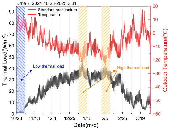
Figure 7.
Hourly thermal load of standard architecture during the heating season.
Figure 7 illustrates the unit-area load (black curve) and ambient temperature (yellow curve) for the standard 4U/6F building during the heating season from 23 October 2024, to 31 March 2025.
During the initial heating phase (late October to early November 2024, denoted by the blue hatched area), ambient temperatures exceeded 0 °C. The unit-area thermal load remained consistently low (0–10 W/m2). As temperatures declined, the mid-heating phase (December 2024 to February 2025) became the core period, exhibiting the season’s lowest ambient temperatures and peak thermal demands. Two distinct temperature minima occurred: 8–14 January 2025; 1–8 February 2025. Both reach valley temperatures of approximately −25 °C. Concurrently, unit-area thermal loads peaked at 40–45 W/m2—the highest values observed in the heating season. The final heating phase (March 2025) saw drastic temperature fluctuations (−10 °C to 15 °C), inducing significant load oscillations (10–20 W/m2).
Figure 8, Figure 9 and Figure 10 demonstrate that room heating loads exhibit strong correlations with spatial positions within buildings. Specifically:
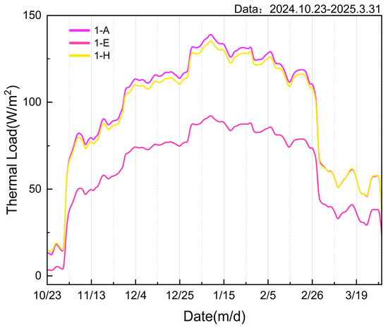
Figure 8.
Daily thermal load of ground-floor rooms during the heating season.
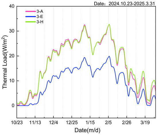
Figure 9.
Daily thermal load of middle-floor rooms during the heating season.
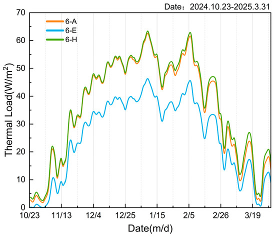
Figure 10.
Daily thermal load of top-floor rooms during the heating season.
- Perimeter rooms (building edges) sustain significantly higher loads than central rooms (building cores);
- Ground-floor rooms experience greater thermal demand than top-floor rooms;
- Middle-floor rooms consistently demonstrate the lowest loads.
Consequently, we propose a hierarchical load calculation framework: building-level loads aggregate all room-level loads. Spatial position-based classification groups rooms with identical load patterns for computational simplification. When internal room structures are invariant, variations in unit count (a) or floor number (b) do not alter positional load patterns.
As a result, the existing computational results can be directly applied to buildings exhibiting comparable spatial typologies. Details of the implementation mechanisms are provided in Section 3.2.
3. Load Calculation
Section 2.3 has established the hourly heating loads for the standard 4U/6F building model. This section conducts a detailed analysis of thermal environment variations experienced by rooms at distinct spatial locations within the apartment. Furthermore, it elucidates the methodology for extrapolating calculated loads from the standard 4U/6F configuration to compute loads for other apartment typologies within the residential community, ultimately enabling community-wide aggregate load synthesis.
3.1. Decoupling of Building Loads
As listed in Table 2, the apartment comprises nine prototypical types of residential rooms.
Table 2.
Information on 4U/6F typical residential rooms.
As specified in Table 2, all Unit A rooms are located at the westernmost building edge, resulting in west-facing walls conducting heat exchange with the external environment; conversely, Unit H rooms positioned on the eastern side exhibit external heat exchange through east-facing walls. Units B-G experience no inter-unit heat transfer across their east–west walls due to stable 18 °C indoor conditions; ground-floor (F1) rooms demonstrate direct floor-to-soil heat exchange given their soil contact, while top-floor (F6) ceilings exchange heat externally since 6F is the building’s uppermost level. Intermediate floors preclude inter-floor heat transfer; north–south heat exchange walls (omitted from tabulation due to universality) and F1’s distinct floor area (80.11 m2 vs. 88.45 m2 for upper floors) invalidate direct load comparisons.
Figure 4 illustrates symmetric floor plans between Unit A (western Unit 1) and Unit H (eastern Unit 4), yielding identical external heat-exchange areas; ground-floor units (F1) contact soil across 80.11 m2, whereas top-floor units (F6) exhibit 88.45 m2 ceiling-level environmental heat transfer.
Figure 11 presents hourly loads of representative rooms simulated by DOE-2 during December 1–20, 2024, where color-coded lines represent distinct room types; all loads exhibit characteristic 24 h cyclic variations, with spatial positioning exerting a significant influence on differences in magnitude.
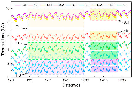
Figure 11.
(12/1–12/20) Typical residential rooms’ thermal loads (kW).
Figure 12 presents hourly thermal loads for representative rooms characterized by distinct spatial thermal patterns during December 1–20. This period was selected due to its stable ambient temperatures (±2 °C diurnal variation), providing optimal conditions for observing hierarchical relationships among positional loads. According to the load distribution shown in Figure 12, the rooms of a building need to be divided into nine categories.
Figure 12.
(12/1–12/20) Typical residential rooms’ thermal loads (W/m2).
Analysis reveals the following:
- The middle-floor intermediate room (F3) exhibits the lowest unit-area load at 12.57 W/m2;
- The top-floor intermediate room (F6) demonstrates a moderate load of 35.19 W/m2;
- The ground-floor intermediate room yields the peak load at 74.58 W/m2.
Spatial patterns are summarized as follows:
- Within a single floor, intermediate rooms sustain minimum thermal loads while perimeter rooms (building edges) bear maximum loads;
- Within the same unit, the sequence of heat loads from largest to smallest is the bottom floor, the top floor, and the middle floor.
3.2. Re-Coupling of Building Loads
Analysis of thermal load data for residential rooms in distinct spatial positions of the reference building reveals a fundamental principle: when indoor temperatures are consistently maintained, rooms within identical thermal environments exhibit identical load patterns. This finding enables the re-coupling of room loads computed for the reference building to derive new building load datasets. The efficacy of this process hinges critically upon the re-coupling computational methodology, the specifics of which are illustrated in Figure 13.
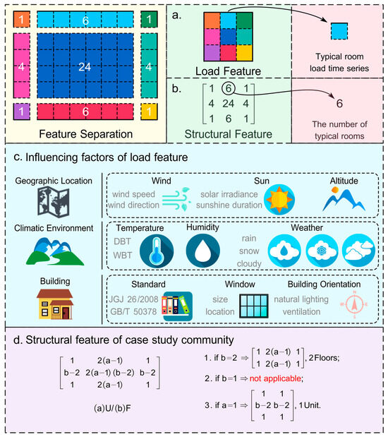
Figure 13.
Method for re-coupling building loads. (a) Load feature matrix (b) Structural feature matrix (c) Influencing factors of load feature (d) Structural feature of case study community.
The spatial configuration of buildings is categorized into nine distinct thermal-environment zones: (1) top-floor west-side households, (2) top-floor middle households, (3) top-floor east-side households, (4) middle-floor west-side households, (5) middle-floor middle households, (6) middle-floor east-side households, (7) ground-floor west-side households, (8) ground-floor middle households, and (9) ground-floor east-side households.
For a representative 4U/6F apartment building with one staircase serving two households per floor, the household distribution across these zones comprises: 1, 6, 1, 4, 24, 4, 1, 6, 1 households, respectively. Hourly loads of these nine prototypical households are represented by distinct colors in the figure, while household counts are encoded within matrices. This process achieves feature separation of heating-season loads, yielding two matrices:
Load Characteristic Matrix (Figure 13a): A 3 × 3 array containing heating-season loads for all characteristic rooms. Solid and dashed boundaries indicate whether walls conduct external heat exchange.
Structural Characteristic Matrix (Figure 13b): Represents architectural typology. Despite diverse building configurations in the case study community, identical external environments permit load calculation for new typologies through mere modification of structural matrix parameters.
Figure 13a,b represent the core of matrix decoupling in the proposed methodology, which decomposes building loads into two key matrices. Figure 13a illustrates the Load Feature matrix, where different colors denote the hourly load profiles of standard rooms across an entire heating season. Essentially, it is the hourly load data corresponding to the room, reflecting the load demand of the room every hour. It is stored in the form of an array. Figure 13b presents the Structural Feature matrix, which quantifies the distribution of corresponding thermal patterns within a building. These two matrices enable accurate reconstruction of building load characteristics. For different building configurations, only the Structural Feature matrix needs to be modified to derive the specific load profile of the new building, a process corresponding to the matrix reconstruction stage in this methodology. Through thermal pattern decoupling and subsequent matrix reconstruction, the proposed approach achieves comprehensive load calculation for all buildings in the case study community, forming the operational core of the methodological framework.
As illustrated in Figure 13c, the Characteristic Load Matrix constitutes the methodological cornerstone of this load calculation framework. This matrix can be acquired through multiple approaches: Empirical measurement of heating network parameters (supply/return water temperatures and flow rates) to derive thermal loads; simulation-based computation of individual room loads; pre-trained machine learning models for room-level load prediction.
Despite comprehensive parameter monitoring in centralized heating systems across northern Chinese cities, household-level load measurement remains challenging, restricting practical deployment of conventional machine learning models due to limited scalability. Our model resolves this by requiring training data from only minimal representative rooms, enabling accurate estimation of building- or community-scale loads with direct comparability to district heating station outputs.
Figure 13c catalogs three primary influence categories:
- a. Climatic & Building-Specific Determinants:
- Wind Effects: Spatial variations in wind velocity modulate wall heat exchange rates; directionality dictates heat transfer differentials across orientations;
- Solar Exposure: Latitudinal position governs received solar radiation intensity and duration;
- Elevation Impacts: Altitudinally induced diurnal temperature gradients redistribute heating plant load allocations.
- b. Climatic & Building-Specific Determinants:
- Thermal Periodicity: Temperature exhibits diurnal/seasonal oscillations, directly dictating load matrix dynamics;
- Humidity-Enthalpy Coupling: Air moisture content affects enthalpy values, critically governing cold air infiltration rates in conventional load calculations;
- Meteorological Modulation: Weather events indirectly recalibrate parameters including ambient temperature, solar irradiance, and air enthalpy.
- c. Architectural Mediators:
- Construction Standards: Temporally evolving building codes fundamentally reconfigure the load matrix;
- Fenestration Properties: Window placement, dimensions, and material composition directly modulate matrix elements;
- Orientation-Driven Exposure: Building alignment governs photoperiod duration and room-specific solar access.
The computational methodology for the structural characteristic matrix is illustrated in Figure 13d. This matrix enables the calculation of quantities for distinct prototypical household types. While this study focuses on buildings with one staircase serving two households per floor, the approach is similarly applicable to structures with alternative layouts (e.g., one-staircase-three-household configurations) through adjustments to matrix dimensions (rows/columns) and recalibration of household counting algorithms based on spatial configurations.
Special cases requiring specific handling include:
- For b = 2 (two-floor buildings), the matrix reduces to 2 × 3 dimensions, retaining only the top-floor and ground-floor strata of the original matrix;
- For b = 1 (single-floor buildings), this methodology is inapplicable due to simultaneous heat dissipation through ceilings and floors. None of the nine predefined prototypical households match this thermal environment, necessitating direct thermal modeling or new machine learning model development;
- For a = 1 (single-household buildings), the matrix transforms into 3 × 2 dimensions, preserving exclusively the eastern and western orientations of the original configuration.
The biggest difference between this method and other methods, and also its most distinctive innovation, lies in the scalability of the calculation results. By analyzing the heating conditions of rooms within buildings with different floor heights and different numbers of units, for similar buildings that meet the conditions, the calculation results of typical buildings can be directly utilized, which reduces a large amount of repetitive work and shortens the calculation time.
3.3. Contrastive Analysis
Decoupling the load characteristics and structural characteristics of the reference building yields two core matrices. For all the buildings within the case area, this method is used to calculate the heating season building load. Subsequent recoupling computations of these matrices enable the determination of thermal loads for all buildings within the residential community, culminating in daily load calculations for the entire heating season. The calculated building loads versus actual supplied heat loads of the case study community are presented in Figure 14.
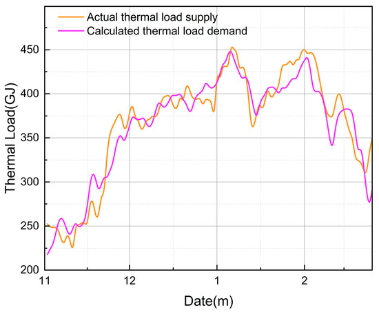
Figure 14.
Comparison of thermal loads in a case study community.
Figure 14 presents a comparison between the actual thermal load supply from the heating station and the calculated thermal load demand derived from our methodology during the heating season. The orange curve represents the actual heat supply, while the purple curve shows the computed demand. Overall, both curves exhibit consistent temporal trends, indicating that the proposed method accurately captures the dynamic behavior of thermal load. Detailed error analysis reveals that the model has a Root Mean Square Error (RMSE) of 24.15 GJ, a Mean Absolute Percentage Error (MAPE) of 4.94%, and a Mean Percentage Error (MPE) of −0.82%, demonstrating high prediction accuracy. In the initial phase, rapid increases in load are observed as the system stabilizes. Three distinct peaks in the mid-phase—occurring on 8–14 January, 1–8 February, and 18–24 February 2025—correspond to Arctic outbreaks and are precisely reproduced by the model. In the final phase, despite a significant reduction in demand due to ambient warming (a monthly mean temperature increase of +4.2 °C), the heating station continued to deliver elevated supply, resulting in an overprovision of 27–33 GJ/day. This highlights the utility of the proposed method in identifying operational inefficiencies and informing real-time regulation strategies.
Figure 15 plots deviations from the fitted line, where outliers primarily originate from abrupt ambient temperature shifts (±7.2 °C/day) during transition periods (1–15 November and 15–31 March). The overall model precision achieves R2 = 0.88, with superior goodness-of-fit during the mid-phase when heat supply concentrates between 350–450 GJ/day. By comparing the calculated heating load obtained using the proposed method for the case study community with the actual measured load, the validity and reasonableness of the method are demonstrated.
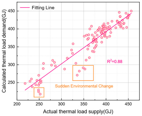
Figure 15.
Scatter plot of actual vs. calculated thermal load with fitting line.
4. Conclusions
This study proposes a spatial pattern decoupling-recoupling methodology for the explicit calculation of building loads. By decoupling building loads based on rooms in distinct thermal environments, we derive two characteristic matrices: the Typical Room Load Matrix (quantifying thermal behavior patterns) and the Building Structural Matrix (encoding spatial configurations).
Structural matrix parameters are calibrated based on architectural typologies. A residential community in Songyuan, Jilin Province, Northeast China (43.88° N, 126.57° E) serves as the validation case. The research examines factors influencing the load characteristic matrix, thermal environmental variations across spatial positions and, discrepancies between computed loads and actual heat supply from district heating stations.
- This research firstly validates the thermodynamic zoning principle for building spaces: structures can be partitioned into nine standardized room categories encompassing top-floor (west/intermediate/east), middle-floor (west/intermediate/east), and ground-floor (west/intermediate/east) spatial units. Energy dissipation analysis shows that energy consumption is lowest in laterally intermediate units and vertically middle floors, owing to thermal buffering and reduced exposure to the building envelope.
- The feasibility of load synthesis via matrix-coupling operations between the load characteristic matrix and structural characteristic matrix is demonstrated. Case validation shows strong alignment between computed and actual heating station supply data (R2 = 0.88, p < 0.001), with an RMSE of 24.15 GJ, a MAPE of 4.94%, and an MPE of −0.82% against actual heating supply data. Peak prediction accuracy is observed in the 350–450 GJ nominal heating range, corresponding to ambient temperatures of −24.3 °C to −18.7 °C during extreme cold episodes.
- The most distinctive innovation of this framework lies in its scalability: once the Typical Room Load Matrix is calibrated using a representative prototype building, it can be directly reused for any building sharing the same construction era, envelope specifications, and room categorization logic—regardless of unit count or floor number. This eliminates the need for repetitive, building-by-building energy simulations. For communities composed of analogous architectural typologies, the method dramatically reduces modeling effort and computational time, while preserving spatial granularity. This capability not only enhances the operational efficiency of load forecasting but also enables seamless integration with smart district heating systems through dynamic matrix updates.
Although the proposed method demonstrates strong performance in rapidly estimating heating loads for existing residential clusters in cold climates, several limitations remain and warrant further investigation and refinement.
First, the current model relies on simplified assumptions regarding internal building spatial layouts—specifically, it assumes uniform functional zoning across rooms. This approach does not adequately account for the heterogeneity of indoor thermal environments arising from variations in apartment layouts, interior partitions, or occupant usage patterns in real-world dwellings. Such an assumption may introduce prediction bias, particularly in highly diverse existing residential clusters. A practical solution that could be explored is to assign building-type-specific adjustment coefficients based on the framework established in this study. These coefficients can be determined using various optimization methods (e.g., genetic algorithms, Bayesian optimization), with model performance metrics—such as RMSE, MAPE, or R2—serving as the optimization objective to identify the coefficient set that yields the most accurate load predictions.
Second, this study focuses exclusively on typical cold-climate regions, where meteorological boundary conditions, heating schedules, and building envelope characteristics exhibit distinct regional traits. Consequently, the generalizability of the proposed model to other climate zones—such as hot-summer/cold-winter, temperate, or tropical regions—has not been validated. Future work should systematically evaluate the model’s transferability across different climate classifications and explore the integration of climate-adaptive parameters or region-specific calibration mechanisms to enable robust cross-regional deployment.
Furthermore, the dynamic influence of occupant behavior—including window opening, appliance usage, and daily activity patterns—is currently modeled using statistical averages or simplified rule-based assumptions, without real-time, individualized coupling. Integrating high-resolution energy consumption data with advanced behavioral modeling techniques represents a promising avenue for enhancing the accuracy and responsiveness of heating load predictions.
In future research, this study will incorporate the impact of thermal performance degradation in building envelopes to enable the model to adapt to post-retrofit thermal load characteristics. By integrating digital twin technology with IoT sensor networks, the methodology will enable real-time monitoring of envelope performance changes (e.g., thermal transmittance degradation) and dynamically update the coefficients in the Load Feature Matrix. For instance, infrared thermography can monitor wall temperature distributions, and when a perimeter unit correction factor is detected to shift from 1.25 to 1.30, the matrix parameters will be automatically recalibrated to enhance computational accuracy. The proposed computationally lightweight approach not only provides an efficient and precise solution for thermal load calculation in existing building clusters but also establishes a methodological foundation for intelligent and low-carbon transitions in building energy systems.
As urban renewal initiatives advance, this methodology will play an increasingly critical role in the renovation of aging residential communities and the development of smart district heating systems. It offers technical support for achieving carbon peaking and carbon neutrality goals in the building sector by bridging the gap between physical building characteristics and scalable energy management solutions.
Author Contributions
Conceptualization, H.C. and X.Y.; methodology, X.Y.; software, Z.L., G.Y.; validation, X.M., J.L. and Z.C.; formal analysis, S.W.; resources, Z.L.; data curation, X.Y.; writing—original draft preparation, X.Y.; writing—review and editing, X.Y.; visualization, W.J.; supervision, G.Y.; project administration, H.C.; funding acquisition, H.C. All authors have read and agreed to the published version of the manuscript.
Funding
This research was funded by The Science and Technology Project of China Huaneng Group: “Research on Key Technologies of Spatiotemporal Characteristics of Complex Heating Energy and Mass Distribution” (Project No. HNKJ23-H60).
Data Availability Statement
All data used to support the findings of this study are available from the corresponding author upon request.
Conflicts of Interest
Authors Haofei Cai, Ziyang Cheng and Guopeng Yao were employed by the company Huaneng Clean Energy Research Institute Co., Ltd. Author Xin Meng was employed by the company Huaneng Jilin Power Generation Co., Ltd. Authors Junjie Liu, Shuming Wang and Wei Jiang were employed by the company Huaneng Songyuan Thermal Power Co., Ltd. The remaining authors declare that the research was conducted in the absence of any commercial or financial relationship that could be construed as a potential conflict of interest.
Glossary
| List of symbols | |
| a | Number of building units (—) |
| b | Number of floors (—) |
| F | Floor count designation (e.g., 6F = six-story building) |
| MAPE | Mean Absolute Percentage Error (%) |
| MPE | Mean Percentage Error (%) |
| Q | Hourly heating load (kW) |
| q | Unit-area heating load (W/m2) |
| R2 | Coefficient of determination |
| RMSE | Root Mean Square Error (GJ) |
| Tin | Indoor setpoint temperature (°C) |
| Tout | Outdoor ambient temperature (°C) |
| U | Building unit count designation (e.g., 4U = four-unit building) |
| BSEI | Building Energy Simulation: An energy consumption calculation software |
| DOE-2 | U.S. Department of Energy Building Energy Simulation Program, Version 2 |
| 4GDH | Fourth-Generation District Heating |
| 5GDH | Fifth-Generation District Heating |
References
- Fan, C.; Yan, D.; Xiao, F.; Li, A.; An, J.; Kang, X. Advanced Data Analytics for Enhancing Building Performances: From Data-Driven to Big Data-Driven Approaches. Build. Simul. 2021, 14, 3–24. [Google Scholar] [CrossRef]
- CABEE. Research Report on Carbon Emissions in the Field of Urban and Rural Development in China (2024 Edition); China Association of Building Energy Efficiency (CABEE) & Chongqing University: Chongqing, China, 2024. [Google Scholar]
- Jiang, Y.; Hu, S.; Liu, X.; Zhang, T.; Wei, Q. Decarbonize Public and Commercial Buildings: China Building Energy and Emission Yearbook 2022; Springer Nature: Singapore, 2023; ISBN 978-981-19552-5-9. [Google Scholar]
- Dang, L.M.; Nguyen, L.Q.; Nam, J.; Nguyen, T.N.; Lee, S.; Song, H.-K.; Moon, H. Fifth Generation District Heating and Cooling: A Comprehensive Survey. Energy Rep. 2024, 11, 1723–1741. [Google Scholar] [CrossRef]
- Lund, H.; Werner, S.; Wiltshire, R.; Svendsen, S.; Thorsen, J.E.; Hvelplund, F.; Mathiesen, B.V. 4th Generation District Heating (4GDH). Energy 2014, 68, 1–11. [Google Scholar] [CrossRef]
- Nielsen, S.; Hansen, K.; Lund, R.; Moreno, D. Unconventional Excess Heat Sources for District Heating in a National Energy System Context. Energies 2020, 13, 5068. [Google Scholar] [CrossRef]
- Yang, T.; Liu, W.; Kramer, G.J.; Sun, Q. Seasonal Thermal Energy Storage: A Techno-Economic Literature Review. Renew. Sustain. Energy Rev. 2021, 139, 110732. [Google Scholar] [CrossRef]
- Sorknæs, P.; Østergaard, P.A.; Thellufsen, J.Z.; Lund, H.; Nielsen, S.; Djørup, S.; Sperling, K. The Benefits of 4th Generation District Heating in a 100% Renewable Energy System. Energy 2020, 213, 119030. [Google Scholar] [CrossRef]
- Buffa, S.; Cozzini, M.; D’Antoni, M.; Baratieri, M.; Fedrizzi, R. 5th Generation District Heating and Cooling Systems: A Review of Existing Cases in Europe. Renew. Sustain. Energy Rev. 2019, 104, 504–522. [Google Scholar] [CrossRef]
- Ahmad, M.W.; Mourshed, M.; Yuce, B.; Rezgui, Y. Computational Intelligence Techniques for HVAC Systems: A Review. Build. Simul. 2016, 9, 359–398. [Google Scholar] [CrossRef]
- Lu, Y.; Tian, Z.; Zhang, Q.; Zhou, R.; Chu, C. Data Augmentation Strategy for Short-Term Heating Load Prediction Model of Residential Building. Energy 2021, 235, 121328. [Google Scholar] [CrossRef]
- Aparicio-Fernández, C.; Vivancos, J.-L.; Cosar-Jorda, P.; Buswell, R.A. Energy Modelling and Calibration of Building Simulations: A Case Study of a Domestic Building with Natural Ventilation. Energies 2019, 12, 3360. [Google Scholar] [CrossRef]
- Tan, X.; Zhu, Z.; Sun, G.; Wu, L. Room Thermal Load Prediction Based on Analytic Hierarchy Process and Back-Propagation Neural Networks. Build. Simul. 2022, 15, 1989–2002. [Google Scholar] [CrossRef]
- Jiang, W.; Wang, P.; Ma, X.; Liu, Y. Development of a Grey-Box Heat Load Prediction Model by Subspace Identification Method for Heating Building. Build. Environ. 2025, 280, 113119. [Google Scholar] [CrossRef]
- Zhang, Q.; Tian, Z.; Ma, Z.; Li, G.; Lu, Y.; Niu, J. Development of the Heating Load Prediction Model for the Residential Building of District Heating Based on Model Calibration. Energy 2020, 205, 117949. [Google Scholar] [CrossRef]
- Afram, A.; Janabi-Sharifi, F. Theory and Applications of HVAC Control Systems—A Review of Model Predictive Control (MPC). Build. Environ. 2014, 72, 343–355. [Google Scholar] [CrossRef]
- Gutiérrez González, V.; Ramos Ruiz, G.; Fernández Bandera, C. Empirical and Comparative Validation for a Building Energy Model Calibration Methodology. Sensors 2020, 20, 5003. [Google Scholar] [CrossRef]
- Wei, Y.; Zhang, X.; Shi, Y.; Xia, L.; Pan, S.; Wu, J.; Han, M.; Zhao, X. A Review of Data-Driven Approaches for Prediction and Classification of Building Energy Consumption. Renew. Sustain. Energy Rev. 2018, 82, 1027–1047. [Google Scholar] [CrossRef]
- Delcroix, B.; Ny, J.L.; Bernier, M.; Azam, M.; Qu, B.; Venne, J.-S. Autoregressive Neural Networks with Exogenous Variables for Indoor Temperature Prediction in Buildings. Build. Simul. 2021, 14, 165–178. [Google Scholar] [CrossRef]
- Xiao, Z.; Zhang, J.; Xiao, F.; Chen, Z.; Xu, K.; So, P.M.; Lau, K.T. An AI-Enabled Optimal Control Strategy Utilizing Dual-Horizon Load Predictions for Large Building Cooling Systems and Its Cloud-Based Implementation. Energy Build. 2025, 330, 115352. [Google Scholar] [CrossRef]
- Bacher, P.; Madsen, H. Identifying Suitable Models for the Heat Dynamics of Buildings. Energy Build. 2011, 43, 1511–1522. [Google Scholar] [CrossRef]
- Li, Y.; O’Neill, Z.; Zhang, L.; Chen, J.; Im, P.; DeGraw, J. Grey-Box Modeling and Application for Building Energy Simulations—A Critical Review. Renew. Sustain. Energy Rev. 2021, 146, 111174. [Google Scholar] [CrossRef]
- Tugores, J.; Macarulla, M.; Gangolells, M. Hybrid Grey Box Modelling of Indoor Air Quality and Thermal Dynamics in Indoor Environments. Energy Build. 2025, 334, 115528. [Google Scholar] [CrossRef]
- Yu, X.; Ren, Z.; Liu, P.; Imsland, L.; Georges, L. Comparison of Time-Invariant and Adaptive Linear Grey-Box Models for Model Predictive Control of Residential Buildings. Build. Environ. 2024, 254, 111391. [Google Scholar] [CrossRef]
- Zhang, H.; Li, Z.; Fan, X.; Duan, D.; Zheng, W. Air-Conditioning Load Characteristics and Grey Box Predicting Model in Subway Stations. J. Build. Eng. 2024, 91, 109656. [Google Scholar] [CrossRef]
- Xie, J.; Li, H.; Hong, T. A Lifelong Meta-Learning Approach for Learning Deep Grey-Box Representative Thermal Dynamics Models for Residential Buildings. Energy Build. 2024, 318, 114408. [Google Scholar] [CrossRef]
- Lin, X.; Tian, Z.; Song, W.; Lu, Y.; Niu, J.; Sun, Q.; Wang, Y. Grey-Box Modeling for Thermal Dynamics of Buildings under the Presence of Unmeasured Internal Heat Gains. Energy Build. 2024, 314, 114229. [Google Scholar] [CrossRef]
- Serasinghe, R.; Long, N.; Clark, J.D. Parameter Identification Methods for Low-Order Gray Box Building Energy Models: A Critical Review. Energy Build. 2024, 311, 114123. [Google Scholar] [CrossRef]
- Jiang, M.; Speetjens, M.; Rindt, C.; Smeulders, D. A Reduced-Order Model for Dynamic Simulation of District Heating Networks. arXiv 2022, arXiv:2211.14119. [Google Scholar] [CrossRef]
- Silvestri, A.; Lydon, G.P.; Waibel, C.; Wu, D.; Schlueter, A. Data-Driven Reduced Order Modelling Using Clusters of Thermal Dynamics. In Proceedings of the Building Simulation 2023: 18th Conference of IBPSA, Shanghai, China, 4–6 September 2023. [Google Scholar]
- Abdel-Jaber, F.; Dirks, K.N. A Review of Cooling and Heating Loads Predictions of Residential Buildings Using Data-Driven Techniques. Buildings 2024, 14, 752. [Google Scholar] [CrossRef]
- Zhang, H.; Hewage, K.; Bakhtavar, E.; Sun, Q.; Sadiq, R. Robust Building Energy Retrofit Evaluation under Uncertainty: An Interpretable Machine Learning Approach. Energy Convers. Manag. 2025, 345, 120362. [Google Scholar] [CrossRef]
- Weber, T.; Schneeberger, S.; Schuetz, P. Estimating Heterogeneous Treatment Effects of Building Energy Efficiency Retrofits Using Machine Learning. Energy Build. 2025, 347, 116369. [Google Scholar] [CrossRef]
- Li, A.; Sun, Y.; Xu, X. Development of a Simplified Resistance and Capacitance (RC)-Network Model for Pipe-Embedded Concrete Radiant Floors. Energy Build. 2017, 150, 353–375. [Google Scholar] [CrossRef]
- Bagheri, A.; Feldheim, V.; Thomas, D.; Ioakimidis, C.S. The Adjacent Walls Effects in Simplified Thermal Model of Buildings. Energy Procedia 2017, 122, 619–624. [Google Scholar] [CrossRef]
- Bueno, B.; Norford, L.; Pigeon, G.; Britter, R. A Resistance-Capacitance Network Model for the Analysis of the Interactions between the Energy Performance of Buildings and the Urban Climate. Build. Environ. 2012, 54, 116–125. [Google Scholar] [CrossRef]
- Hu, Z.-A.; Li, J.; Nie, Z. Long Live Friendship? The Long-Term Impact of Soviet Aid on Sino-Russian Trade. J. Dev. Econ. 2023, 164, 103117. [Google Scholar] [CrossRef]
- Lin, T.; Qian, W.; Wang, H.; Feng, Y. Air Pollution and Workplace Choice: Evidence from China. Int. J. Environ. Res. Public Health 2022, 19, 8732. [Google Scholar] [CrossRef] [PubMed]
- Xinhua China Unveils Policies to Revitalize Northeast. Available online: https://www.chinadaily.com.cn/bizchina/2014-08/20/content_18452308.htm (accessed on 13 May 2025).
- Gang, W.; Wang, S.; Xiao, F.; Gao, D. District Cooling Systems: Technology Integration, System Optimization, Challenges and Opportunities for Applications. Renew. Sustain. Energy Rev. 2016, 53, 253–264. [Google Scholar] [CrossRef]
- Lab, L.B.; Hirsch, J.J. DOE-2 Engineers Manual Version 2.1A; Los Alamos Scientific Laboratory: Los Alamos, NM, USA, 1980. [Google Scholar]


Disclaimer/Publisher’s Note: The statements, opinions and data contained in all publications are solely those of the individual author(s) and contributor(s) and not of MDPI and/or the editor(s). MDPI and/or the editor(s) disclaim responsibility for any injury to people or property resulting from any ideas, methods, instructions or products referred to in the content. |
© 2025 by the authors. Licensee MDPI, Basel, Switzerland. This article is an open access article distributed under the terms and conditions of the Creative Commons Attribution (CC BY) license (https://creativecommons.org/licenses/by/4.0/).