Abstract
This study presents a novel solid oxide electrolysis cell (SOEC) design with variable channel widths to optimize thermal management and electrochemical performance for enhanced hydrogen production. Using high-fidelity computational modeling in COMSOL Multiphysics 6.1, five distinct channel width configurations were analyzed, with a baseline model validated against experimental data. The simulations showed that modifying the channel geometry, particularly in Scenario 2, significantly improved hydrogen production rates by 6.8% to 29% compared to a uniform channel design, with the effect becoming more pronounced at higher voltages. The performance enhancement was found to be primarily due to improved fluid velocity regulation, which increased reactant residence time and enhanced mass transport, rather than a significant thermal effect, as temperature distribution remained largely uniform across the cell. Additionally, the inclusion of a dedicated heat transfer channel was shown to improve current density and overall efficiency, particularly at lower voltages. While a small increase in voltage raised internal cell pressure, the variable-width designs, especially those with widening channels, led to greater hydrogen output, albeit with a corresponding increase in system energy consumption due to higher pressure. Overall, the findings demonstrate that strategically designed variable-width channels offer a promising approach to optimizing SOEC performance for industrial-scale hydrogen production.
1. Introduction
To address the challenge of reducing CO2 emissions in energy-intensive industries such as steelmaking—which account for nearly 7% of global emissions and heavily depend on hydrogen—it is essential to develop alternatives to fossil fuel–based reformers [1,2,3]. Hydrogen production through electrolysis technologies, including solid oxide electrolysis cells (SOECs, 700–900 °C) [4], proton exchange membrane (PEM, 100–150 °C) [5], and alkaline (AK, 60–120 °C) [6] electrolyzers, provides a sustainable option compared with conventional steam methane reforming (SMR) [7]. Unlike SMR, which consumes fossil fuels and generates 9–12 kg of CO2 per kilogram of hydrogen [8], electrolysis relies solely on water and electricity, producing no direct carbon emissions when powered by renewable energy sources [9]. Moreover, because water electrolysis becomes increasingly endothermic at elevated temperatures, SOECs can effectively utilize external heat from renewable sources such as solar thermal, wind, or nuclear energy, thereby lowering the electrical energy demand for hydrogen generation [10,11].
Recent progress in SOEC research has centered on optimizing flow configurations—namely co-flow, counter-flow, and cross-flow—to improve thermal uniformity and hydrogen generation. Using coupled CFD and FEM simulations, Lim et al. [12] showed that non-uniform temperature gradients intensify stress concentrations, especially at interfaces between materials with different thermal expansion coefficients. Their analysis revealed that around 85% of the irreversible heat is generated by activation overpotentials in the fuel and air functional layers and ohmic losses from oxygen ion transport under conditions of 0.6944 A/cm2 current density, 1.418 V cell voltage, and 600 °C inlet temperature. Xu et al. [13] develop a 3-D multi-stack SOEC model to examine electrolysis performance and coupled electricity–heat–gas fields across six stack arrangements, evaluating uniformity with dedicated indices and dimensionless metrics. Similarly, Wang et al. [14] used 3D modeling to demonstrate that optimized flow field configurations enhance both heat and mass transfer, resulting in more uniform temperatures and higher hydrogen yields.
The same interesting ideas for channel changes can be found in other articles. Der and Bertola [15] experimentally mapped co-current oil–water flow in a horizontal serpentine microchannel using high-speed imaging while independently varying the phases’ superficial velocities. They show that curvature-induced secondary flows shift flow-pattern transition boundaries compared with straight channels, yielding a distinct flow-pattern map relevant to mixing and residence-time control. The authors fabricate the device by cutting the serpentine path in a black polypropylene sheet, sandwiched between transparent polypropylene layers and bonded by selective laser welding, enabling clear optical access while maintaining robust sealing. By systematically scanning flow-rate pairs, they construct a flow-pattern map specific to the serpentine layout, demonstrating how curvature promotes enhanced interfacial deformation and mixing and thus alters transition thresholds. Overall, the work shows that channel curvature is a first-order design variable for controlling immiscible two-phase microflows, with direct implications for microfluidic mixing, residence-time management, and phase-contact engineering. Alexander et al. [16] investigated immiscible oil–water plug flow in serpentine microchannels with multiple high-curvature bends (β = 1) at an ultra-low viscosity ratio (λ = 0.001), showing that curvature-driven acceleration/deceleration elongates plugs linearly with capillary number and can even cause plug rupture. Alexander et al. further used laser-induced fluorescence and particle-tracking velocimetry to reveal curvature-induced vortices in aqueous plugs and curvature-dependent structures in oil slugs, defining operating windows that enhance mixing and mass transfer.
Recent studies have started to close this research gap by integrating electrochemical potential distribution and degradation kinetics into their analyses. Virkar et al. [17], in a seminal contribution, developed an analytical framework that captures the spatial variations of electronic potential, oxygen chemical potential, and the resulting interfacial oxygen partial pressure across the electrolyte. This model established the thermodynamic basis for evaluating delamination mechanisms. Building on this, Udagawa et al. [18] modeled a cathode-supported intermediate-temperature SOEC designed for steam electrolysis. Their steady-state simulations showed that at an operating current density of 7000 A/m2 and a steam inlet temperature of 1023 K, the stack required approximately 3 kWh per Nm3 of hydrogen produced—substantially lower than the energy consumption of conventional low-temperature electrolyzers. This underscores the superior efficiency of intermediate-temperature SOECs (IT-SOECs) for hydrogen production. In another study, Zeng et al. [19] analyzed the effect of anode porosity on thermal stress patterns in a planar anode-supported SOFC. They found that porosity strongly influences both the magnitude and distribution of thermal stresses, with higher porosity levels (30–40%) lowering stresses by as much as 25% compared to lower porosity ranges (10–20%).
These papers review the materials, synthesis, mechanisms, and system integration of advanced solid oxide fuel cells (SOFCs) and solid oxide electrolysis cells (SOECs) [20,21,22,23,24,25,26,27,28]. Zhu et al. [29] presented a hybrid modeling approach to optimize the dynamic performance of solid oxide electrolysis cells (SOECs) and demonstrated that allowing for a slight deviation from thermal neutrality can enhance overall efficiency and reduce the cost of syngas production. To produce syngas, the total conversion rate is highest at thermal neutrality, but absorbing a small amount of heat actually boosts overall efficiency to 83.9% and lowers the production cost to just $0.31 per kilogram. Liang et al. [30] proposed a new control strategy for solid oxide electrolysis cells (SOECs) that adjusts the steam flow rate to neutralize internal heat, effectively stabilizing cell temperature and maintaining high efficiency despite rapid fluctuations in solar power. Their results showed that conventional control strategies, which increase airflow rates, are inadequate in effectively suppressing the rate of temperature variation in scenarios of drastic changes in solar power. The novelty of this study lies in being the first to systematically introduce and analyze variable channel-width designs in planar solid oxide electrolysis cells (SOECs) to optimize for both maximum hydrogen production.
This work is, to the best of our knowledge, the first systematic SOEC study of variable-width (tapered) channels as a design lever for residence-time control and maldistribution mitigation, evaluated alongside a dedicated heat-transfer channel in a single multiphysics framework. In contrast to recent flow-field studies that modify waviness or cross-sectional shape to boost mass/heat transfer, we vary the channel width along the flow path and show that widening profiles can lower outlet velocity, raise residence time, and increase H2 production without materially changing temperature uniformity.
2. Materials and Methods
2.1. Geometry Model
This study investigates a novel variable channel width SOEC design to optimize thermal management and electrochemical performance. The cell’s multi-layered structure, illustrated in Figure 1, includes interconnectors, cathode and anode gas diffusion layers (AGDLs) and electrodes (AGDEs), an electrolyte membrane, and a dedicated heat transfer channel. The materials employed are Ni-stabilized ZrO2 (Ni-YSZ) for the anode AGDL/AGDE, Sr-doped LaMnO3 (LSM) for the cathode CGDL/CGDE, Y2O3-stabilized ZrO2 (8YSZ) for the electrolyte, and stainless steel for the separator. The analyzed SOEC has an active area of 64 mm × 60 mm. The electrolyte and both GDEs have a uniform thickness of 15 μm, while the cathode and anode AGDL-CGDL are 50 μm and 25 μm, respectively. All channels are designed in a spiral configuration. To evaluate the impact of channel geometry on performance, five distinct width configuration scenarios were designed, moving beyond a simple uniform design. The base geometry (Scenario 1), shown in Figure 1, features a cathode channel width of 0.8 mm, an anode channel width of 1 mm, and corresponding rib widths of 1 mm and 2 mm. As can be seen in Figure 2, The subsequent scenarios systematically vary these cathode and anode channel and rib widths to assess their influence on gas distribution, pressure drop, and reaction kinetics. The flow in each of the 20 parallel channels per inlet is routed through semicircular paths to minimize pressure drop. The complex geometry, particularly in the variable-width scenarios, required high-fidelity computational modeling. The design was analyzed using COMSOL Multiphysics 6.1. A mesh independence study was conducted, resulting in a high-resolution mesh with approximately 580,000 elements for the base model (Figure 1), with key parameters like porosity, tortuosity, and density detailed in Table 1. The computational intensity of the models necessitated the use of a supercomputer equipped with 7 terabytes of memory to obtain converged and accurate results. By analyzing these variable-width configurations and flow directions, this study provides critical insights into optimizing flow paths and geometry in industrial-scale SOECs to enhance hydrogen yield and overall system efficiency. As can be seen in Figure 3, the channel widths varied using an arithmetic progression, starting from a minimum value of 0.2 Wch. To isolate residence-time effects, we imposed an arithmetic progression of channel widths along the flow direction, generating five scenarios that span the practical tapered-channel space (uniform baseline; monotonic widening; monotonic narrowing; symmetric wedge; piecewise step). Such geometric grading is informed by serpentine-channel literature where curvature-driven secondary flows and local acceleration/deceleration strongly affect mixing and interfacial transport, thereby shaping residence-time distributions.
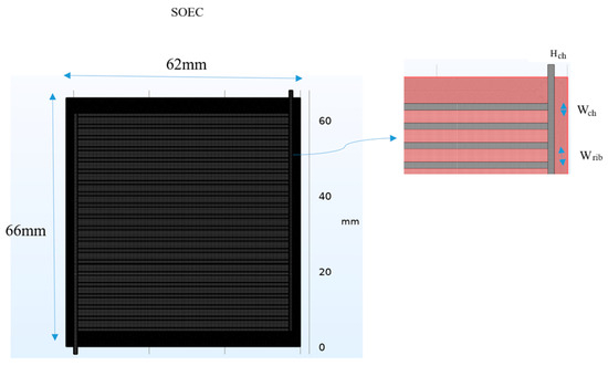
Figure 1.
Schematic of the base SOEC model (Scenario 1) mesh structure and key geometric parameters.
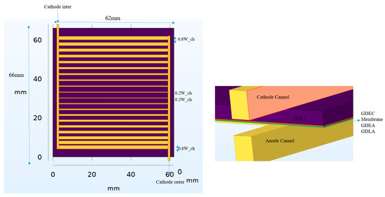
Figure 2.
Cross-sectional view of the multi-layer SOEC structure and gas flow configurations (Scenario 5 example).

Table 1.
Key parameters for CGDL, CGDE, AGDL, AGDE, and electrolyte membrane.
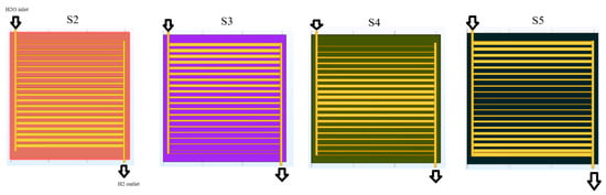
Figure 3.
Cross-sectional view of the multi-layer SOEC structure and gas flow configurations (Scenario 5 example).
2.2. Electrochemical Model
The electrochemical behavior of the SOEC is described by the relationship between the output voltage V, the open circuit voltage VOC, and the various voltage losses (overpotentials), expressed as [31]:
The open circuit voltage VOC is calculated based on the Nernst equation, which accounts for temperature and partial pressures of reactants and products [31]:
The voltage losses, or overpotentials, as divided into activation, ohmic, and concentration components, are calculated as follows:
Activation overpotential at the anode and cathode:
Ohmic overpotential due to ionic and electronic resistances:
Concentration overpotential arising from mass transport limitations:
As shown in Equations (7) and (8), the volumetric current densities at the anode (J1) and cathode (J2) are determined by the Butler–Volmer equations, which describe the electrode kinetics as a function of overpotential [32]:
2.3. Momentum Conservation Model
The momentum transfer within the SOEC is governed by the steady-state Navier–Stokes and continuity equations (Equations (9) and (10)) for ideal gas flow in the channels and Darcy’s law within the porous electrodes. While gas flows through both the electrode channels and their porous structures, the hermetically separated additional channel does not participate in mass transfer to the electrolyte [31]:
Within the porous electrodes, where chemical reactions consume and produce species and the porous matrix imposes flow resistance, the Darcy–Brinkman equations govern gas flow. This model extends Darcy’s law by incorporating viscous shear stress effects to accurately describe momentum transport. The governing equation is given by [31]:
Here κ is the permeability of the porous medium, and other symbols retain their usual meanings. This approach captures the combined effects of pressure gradients, viscous forces, and porous resistance on the gas flow within the electrodes, providing a more accurate representation of momentum conservation in the SOEC porous layers.
Mass transport within the SOEC, driven by convection and diffusion, is modeled using the Maxwell–Stefan equations. In multicomponent gas mixtures, the diffusive flux of one species depends on frictional (momentum-exchange) interactions with all the others. The Maxwell–Stefan (MS) equations capture this coupling and reduce to Fick’s law only in special limits (binary mixture, dilute species, or when cross-coupling is negligible). MS is therefore the consistent choice for high-temperature H2–H2O transport in SOEC channels and porous electrodes, where counter-diffusion and baro/thermo-diffusion can matter. To accurately capture the distinct structural properties of the anode, cathode, additional channel, and porous electrodes, as well as the influence of electrochemical reactions, a specific form of these equations is applied to each region as follows [11]:
For three channels,
For porous electrodes (MS with porous corrections and reaction sources),
where is the mole fraction, which can be figured out from the following equation:
In this study, the thermal diffusion coefficient () is neglected (set to zero). Instead, the effective diffusion coefficient () accounts for microstructural effects in the porous electrodes and accounts for reduced cross-section and tortuous paths:
Many SOEC works use a Bruggeman form ; linear is also standard if τ is calibrated. State which you use and give values. For an N-component mixture, MS uses binary gas diffusivities Dmn(T,p) to build the MS resistance matrix, then solves a small linear system to get fluxes. Many codes (including COMSOL’s Transport of Concentrated Species with “Maxwell–Stefan diffusion”) do this under the hood once you provide Dij(T). In porous zones, you simply replace Dij→Dij,eff.
2.4. Heat Transfer Model
The SOEC heat transfer model focuses on conduction and convection, which are the dominant mechanisms for predicting temperature distribution and enabling thermal management at typical operating temperatures (~800 °C). Boundary and initial parameters like mass flow, oultlet pressure, inlet temperature and inlet gas compositions are showed in Table 2. Although radiation is neglected in this analysis, the thermal behavior of all components—including interconnectors, gas channels, electrolyte, and seals—is governed by the energy balance equations detailed in [11].
Table 2.
Boundary and initial parameters [33].
The heat generation term Qh consists of two components: Qj, which represents the Joule heating resulting from charge transport within the electrical components, and Qe, which accounts for the heat effects related to the endothermic chemical reactions and activation overpotentials. Therefore, the total heat source term Qh can be expressed as [11]
We neglect radiative heat transfer in this single-cell model because, under our operating conditions, its net contribution is small compared with conduction through the interconnects and convection in the gas channels.
Table 3 summarizes the thermo-mechanical properties used for the SOEC thermal analysis across the main components: porous electrodes (GDL/GDE) on the cathode and anode, the dense electrolyte, and the metallic interconnector. The electrodes are modeled with modest thermal conductivity (4 W·m−1·K−1) and typical ceramic-like stiffness (E = 220 GPa cathode, 160 GPa anode) and Poisson’s ratio 0.3, reflecting their porous composite nature. The electrolyte has lower thermal conductivity (2 W·m−1·K−1) but high stiffness (205 GPa), consistent with a dense ceramic that conducts heat less efficiently than the interconnector; the interconnector, by contrast, is the primary heat spreader (k = 30 W·m−1·K−1) with metal-like elasticity (E = 205 GPa). Coefficients of thermal expansion are in a narrow range (≈10.3–12.5 × 10⁻⁶ K−1), which helps limit thermal-mismatch stresses at operating temperature; among them, the electrolyte exhibits the lowest CTE (10.3 × 10⁻⁶ K−1), while the cathode CGDL/CGDE is the highest (12.5 × 10⁻⁶ K−1), guiding expectations for interfacial stress and warpage during heat-up and load transients. Only the boundary and initial conditions are given in Table 4. Other model parameters (such as thermoelectric properties and transfer coefficients) are given in the tables related to the material properties.
Table 3.
SOEC parameters for thermal analysis.
Table 4.
Boundary and initial condition for al scenarios.
3. Results
Prior to analyzing the novel cell design, the baseline SOEC computational fluid dynamics (CFD) model was validated against the experimental data of Momma et al. [34]. As shown in Figure 4, the simulated performance curves at 900 °C and 1000 °C demonstrate strong agreement with the experimental results, with marginal deviations of 3.4% and 6.5%, respectively. These differences fall within an acceptable range, confirming the model’s accuracy. The computational domain was discretized with a predominantly structured mesh comprising ≈ 5.74 × 10⁵ cells in the baseline case. Of these, ≈ 1.67 × 10⁵ were prisms used to resolve near-wall and layered regions, and the remainder were hexahedra in the bulk. To capture steep gradients at solid–electrolyte interfaces, we applied targeted refinement in all electrochemically critical zones—namely the membrane and the gas-diffusion electrodes (cathode/anode, GDEc_\mathrm{c}c, GDEa_\mathrm{a}a). Each porous layer and the membrane were resolved with at least five elements across the through-thickness, and boundary-layer stacks were grown with a smooth growth rate ≤ [1.20–1.25] from the interfaces. Global mesh quality was monitored using standard metrics: the cell aspect ratio distribution was centered around [AR50_{50}50 ≈ …] with max ≤ […], skewness remained low (median ≈ […], max ≤ […]), and orthogonality was ≥ […] for [>99%] of cells. To verify mesh independence, we repeated all simulations on a refined mesh (~1.5 × 10⁶ cells); differences in key integral and local metrics (e.g., cell-averaged membrane overpotential, area-averaged current density at the electrodes, and peak temperature) were <1% relative to the baseline mesh. These results indicate that the reported solutions are mesh-independent within the stated tolerances. A mesh-refinement study (≈5.7 × 10⁵ to ≈1.5 × 10⁶ cells) changed the area-averaged current density, peak temperature, and outlet hydrogen mole fraction by <1%; we therefore Unum≈1% for these observables. To assess model-input uncertainty, we performed one-at-a-time (OAT) ±10% variations around nominal values for porosity ε, tortuosity τ, permeability k, exchange current density i0, inlet temperature Tin, and inlet mass flow. The resulting changes in H2 remained within ±(2–6)% under representative operating conditions.
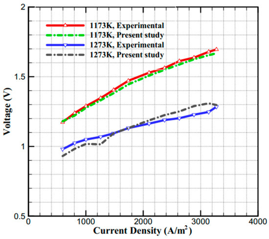
Figure 4.
The comparison of the Voltage–Current Density curves from the model simulations and results from Ref. [34].
This study evaluated the hydrogen production performance of a novel solid oxide electrolysis cell (SOEC) with a variable channel width design, analyzing five distinct flow direction scenarios under adiabatic conditions. The operating conditions were carefully designed to manage the cell’s thermal state. The cathode inlet stream for all scenarios consisted of a 40% H2/60% H2O mixture at 600 °C, while the anode inlet was supplied with a 79% N2/21% O2 mixture at the same temperature. To provide the necessary energy for the endothermic electrolysis reaction, superheated steam at 900 °C was introduced through the additional channel. This established a significant thermal gradient from a reference operating temperature of 800 °C, a strategy intended to supply high-grade heat for efficient electrolysis while using the cooler electrode inlets to reduce thermal stresses and improve the cell’s structural integrity. The results, particularly the molar hydrogen production rates across the cell bed for scenarios 1 and 2 at voltages of 1.1 V, 1.2 V, and 1.3 V (Figure 5), revealed a superior performance for Scenario 2. The hydrogen production rates for Scenario 2 were 0.47, 0.58, and 0.70 at 1.1 V, 1.2 V, and 1.3 V, respectively. These values represent significant performance enhancements of approximately 6.8%, 20.8%, and 29% over the base case (Scenario 1), which recorded rates of 0.44, 0.48, and 0.54 at the same voltages. This trend indicates that the positive effect of the specific channel width modification in Scenario 2 becomes more pronounced at higher operating voltages. A comparison of the hydrogen molar fraction across all five scenarios and three voltages (Figure 6) confirms that production increases with voltage for all designs. Among them, Scenarios 2 and 4 demonstrated the highest performance. The superior results of Scenarios 2 and 4 suggest that a strategic change in channel width, particularly one that increases along the flow path, significantly enhances hydrogen production. This is likely because a widening channel improves gas distribution, reduces pressure drop, and optimizes the residence time of reactants over the electrode surface, thereby improving the electrochemical reaction kinetics. This effect is amplified at higher voltages, where reaction rates are greater.

Figure 5.
Molar fraction of hydrogen for two scenario 1 and 2 for three voltages 1.1, 1.2 and 1.3 V.
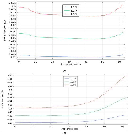
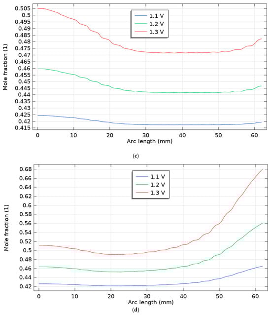
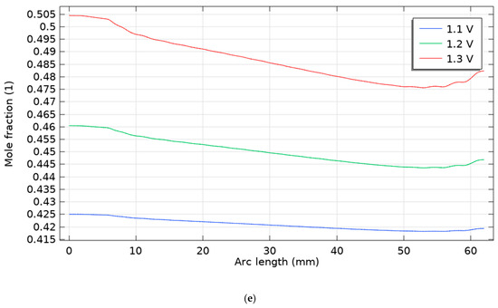
Figure 6.
Molar fraction of hydrogen for five scenarios for three voltages 1.1, 1.2 and 1.3 V, (a) scenario 1, (b) scenario 2, (c) scenario 3, (d) scenario 4, (e) scenario 5.
As shown in Figure 7, at higher drive voltages (1.4–1.5 V), the hydrogen mole-fraction profiles diverge noticeably between the two scenarios. Scenario 1 (first figure) remains nearly uniform along the channel: both curves begin near ~0.54–0.60, show a shallow mid-channel dip, and recover only modestly toward the outlet, with 1.5 V consistently offset above 1.4 V by a nearly constant gap—i.e., voltage mainly raises the baseline level rather than steepening the axial gradient. In contrast, Scenario 2 (second figure) exhibits a monotonic enrichment: starting near ~0.56 (1.4 V) and ~0.60 (1.5 V), the profiles climb steadily with arc length, reaching ~0.79 and ~0.93, respectively, indicating stronger reactant conversion and a much higher voltage sensitivity of the axial composition. When compared with the lower-voltage cases (1.1–1.3 V; see previous figures), both scenarios follow the same qualitative ordering—higher voltage → higher H2 mole fraction everywhere—but the magnitude of change with position is small in Scenario 1 and becomes progressively amplified in Scenario 2. These results suggest that the operating configuration in Scenario 2 enhances transport/kinetics sufficiently that increasing the voltage not only elevates the overall H2 level but also drives a pronounced axial build-up, whereas Scenario 1 remains diffusion-limited and closer to a flat profile even at 1.5 V.
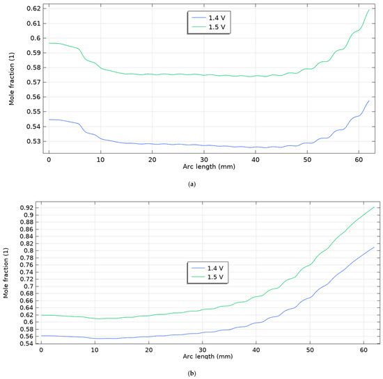
Figure 7.
Molar fraction of hydrogen for five scenarios for voltages of 1.4 and 1.5 V for (a) scenario 1, (b) scenario 2.
As illustrated in Figure 8, the average flow velocity at the outlet channel is compared for Scenarios 1 and 2 at three different voltages (1.1 V, 1.2 V, and 1.3 V). According to the results, the average outlet velocity in Scenario 2 is significantly lower than in Scenario 1. This reduction in flow velocity allows for a longer residence time of reactants within the electrolysis zone, thereby improving electrolysis efficiency and ultimately leading to higher hydrogen production. Specifically, in Scenario 1, the gas velocity decreases from a maximum of 9 m/s to approximately 1.5 m/s at the outlet. In contrast, Scenario 2 exhibits a more substantial reduction, from an initial 9 m/s to nearly zero at the outlet. This pronounced decrease in velocity enhances mass transport and promotes more complete electrochemical reactions, serving as a key factor in increasing hydrogen yield. Under these conditions, the channel Reynolds number remains Re≲102, confirming laminar flow; a k–ω SST test produced <1% changes in Δp.
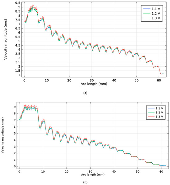
Figure 8.
Fluid velocity changes inside the cathode channel: (a) scenario 1, (b) scenario 2.
We performed a simple energy audit to verify that the geometric benefits are not offset by parasitic pumping work. Using the modeled pressure drop and bulk speed at the channel inlet, the pumping power density was estimated as Ppump′ = Δp u/ηfan. For a representative operating point (Δp = 180, u = 0.7 m·s−1, ηfan = 0.6), this yields Ppump′ ≈ W·m−2. The outlet hydrogen chemical power density was computed from the molar flux, PH2′ = NH2 HHV, with NH2 = 0.68 mol·m−2 s−1 and HHV = 241.8 kJ·mol−1, giving PH2′ ≈ 1.64 × 10⁵. The resulting figure of merit,
indicates that the chemical power of the produced H2 exceeds the parasitic pumping power by roughly three orders of magnitude at this condition. This ratio is area-independent (assuming inlet and outlet areas are comparable), so it provides a robust check that the variable-width designs are not trading performance for excessive pressure drop. Importantly, this audit does not represent overall SOEC efficiency, since the dominant input remains the stack electrical power for electrolysis; rather, it isolates the geometric contribution to auxiliary loads. In our operating window, modest changes to Δp and u from tapering have a negligible impact on net energy when compared to the hydrogen energy output, supporting the industrial feasibility of implementing variable-width channels without incurring meaningful pumping penalties.
Table 5 quantifies the flow and mass-transfer behavior across the ten channels of scenario 4 by reporting the centerline Reynolds number Re = ρUDh/ and the interface Sherwood number Sh = NAL/(DAB Δc). As the channel hydraulic diameter and bulk velocity decrease from channel 1 to channel 10, Re drops from ~60 to <2, confirming fully laminar conditions throughout. Despite the declining velocity, Sh increases modestly along the array because the combined effect of geometry (shorter diffusional path) and the assumed property trend (slightly smaller DAB downstream) raises the normalized interfacial transfer coefficient hm. Together, these metrics show that scenario 4 achieves residence-time control (low Re) without sacrificing interfacial mass transfer (stable/increasing Sh), supporting the design premise that tapered channels can improve utilization while keeping transport favorable.
Table 5.
Reynolds and Sherwood Numbers for Scenario 4 (Channels 1–10).
Figure 9 presents the 3D temperature distribution of the SOEC for Scenarios 1, 2, and 3 at applied voltages of 1.1 V and 1.3 V (the boundary conditions for the cathode, anode, and additional channels remained unchanged). One objective of this analysis was to demonstrate that, despite the cell’s compact size (64 mm × 60 mm with a width of only 2.518 mm), a considerable temperature variation exists across the cell domain. The simulation results clearly indicate that even in such a small structure, a non-uniform temperature distribution is evident; however, this distribution tends to become more uniform with increasing voltage. In Scenario 1, the cell temperature not only increases with higher voltage but also shows a move towards uniformity, with maximum temperatures of 837 K and 879 K at 1.1 V and 1.3 V, respectively. Critically, the results show that changes in the channel cross-section have little impact on the temperature distribution. It can therefore be concluded that the primary reason for the increased molar hydrogen production in Scenarios 2 and 4 is the effective regulation of fluid velocity within the channel, which enhances residence time and mass transport, rather than a thermal effect.
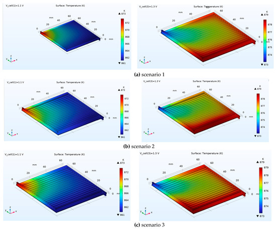
Figure 9.
3D temperature distribution of the SOEC for scenarios 1, 2, and 3 at applied voltages of 1.1 V and 1.3 V.
In Scenario 2, the three-dimensional temperature field remains smooth and predominantly aligned with the channel direction, with a clear streamwise rise from the inlet plenum (cool end) toward the outlet. At 1.4 V (Figure 10a), temperatures span roughly 873–928 K, producing a moderate axial gradient while preserving good lateral uniformity across neighboring channels (only weak banding associated with the rib/channel pattern). Raising the drive to 1.5 V (Figure 10b) amplifies Joule and reaction heat release, broadening the range to ≈ 872–997 K and steepening the axial gradient; peak temperatures shift to the downstream corner near the outlet manifold, consistent with higher current density and longer residence for heat accumulation. Despite the overall increase, the field remains free of localized hot spots within the active area, indicating that Scenario 2’s flow/geometry provides effective transverse heat spreading while voltage primarily controls the magnitude, not the shape, of the temperature distribution.
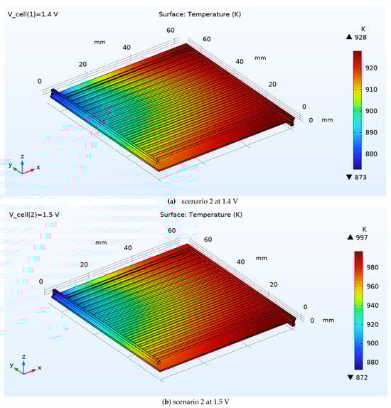
Figure 10.
3D temperature distribution of the SOEC for scenario 2 at 1.4 V and 1.5 V.
As shown in Figure 11, the current density distribution at the CGDL cathode and CGDE cathode junction has been investigated for scenario 1 at two operating voltages of 1.1 V and 1.3 V. Under constant voltage conditions, it is observed that the maximum current density had increased from 2100 A/m2 in voltage 1.1 to 7940 A/m2 in voltage 2. Also in scenario 1, a large cross-sectional area of the SOEC cell is involved in the high-density current (red line), which indicates an improvement in the current distribution and an increase in the efficiency of the electrolyzer in this case. These results indicate that adding a thermal channel to the cell design can improve heat dissipation and, as a result, reduce the ohmic resistance and increase the current density of the SOEC cell. Considering the positive correlation between the operating voltage and current density, increasing the voltage from 1.1 V to 1.3 V leads to a significant increase in the current density and, in addition to the value, a large area of the SOEC cell cross-section is also involved in the higher current. At 1.3 V, the current density in scenario 1 reaches a maximum of 7940 A/m2. Although this increase is relative and limited at high voltages, at lower voltages, the effect of adding a channel in SOEC is much more dramatic, such that it can increase the current density by about 100%. These findings show that proper thermal design, especially at low operating voltages, plays a key role in improving the performance and efficiency of the electrolyzer cell.
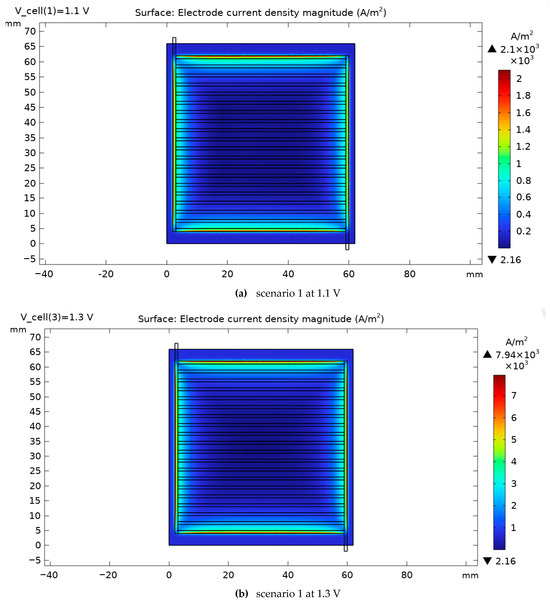
Figure 11.
Electrode current density magnitude for scenario 1 for two voltages, 1.1 and 1.3 V.
The pressure variation on the cathode side for scenarios 1 and 2 is shown in Figure 12 and Figure 13. Increasing the voltage from 1.1 to 1.3 V leads to an increase in the current density and hydrogen gas production on the cathode side. As illustrated in the comparison between Figure 9 and Figure 10, an increase in operating voltage results in a rise in cell pressure from 180 Pa to 183 Pa. This initial pressure increase is primarily a consequence of enhanced electrochemical activity, which leads to a higher rate of hydrogen gas production at elevated voltages. Furthermore, the data from Figure 10 demonstrates that modifications to the cell’s cross-sectional area induce a more substantial pressure increase, reaching 193 Pa. This represents a significant 7% rise compared to the baseline. Consequently, it can be concluded that Scenarios 2 through 5 will be characterized by a greater hydrogen output, a correspondingly higher internal pressure, and an associated increase in the system’s energy consumption. Gas compressibility and mixture state. Gas phases are treated as ideal, low-Mach compressible mixtures. The local density is evaluated from the mixture state as . Transport properties and enter the momentum and species equations in the channel domains; the porous electrodes/GDLs use a Darcy–Brinkman form with the same state-dependent properties. The flow remains subsonic with Ma ≪ 0.3, so compressibility appears through property variation without acoustic effects.
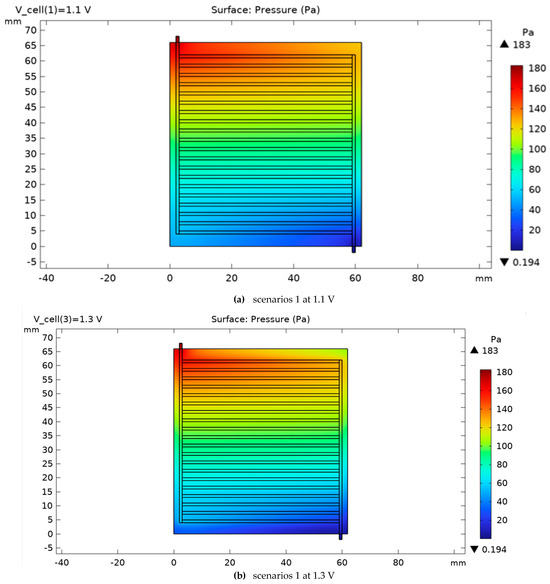
Figure 12.
The pressure variation on the cathode side for scenarios 1 for two voltages, 1.1 and 1.3 V.
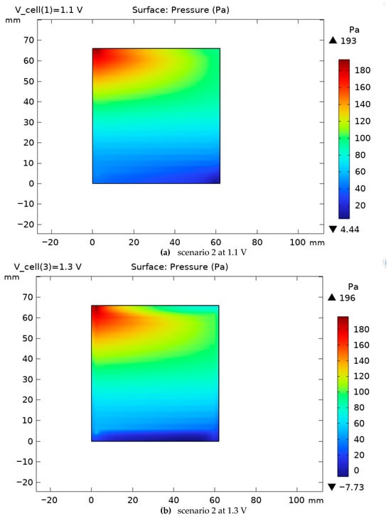
Figure 13.
The pressure variation on the cathode side for scenario 2 for two voltages, 1.1 and 1.3 V.
Acorrdong to Figure 14, porosities of the gas-diffusion layers and electrodes—por1 (CGDL), por2 (GDEC), por3 (GDEA), and por4 (AGDL) together with their corresponding permeabilities (per1–per4), were systematically varied. The outlet hydrogen mole fraction increases monotonically with porosity and, for the outlet-side CGDL-AGDL, decreases with permeability (i.e., lower k yields higher xH2 Specifically, when all porous layers are set to ε = 0.5 (red curve) and the outlet CGDL-AGDL permeability is k = 10−12, the profile shows the highest enrichment along the channel, with the largest separation emerging near the outlet. Physically, higher ε reduces tortuosity and raises the effective diffusivity and accessible TPB area, thereby lowering concentration polarization and improving reactant/product transport through CGDL/CGDE/AGDE. In parallel, a smaller k in AGDL suppresses cross-flow/bypass and increases the local residence time, which promotes conversion and accumulates H2 toward the outlet—hence the steeper terminal rise of the red curve. The near-inlet overlap of all curves indicates a kinetics-dominated region where transport resistances are weak; sensitivity grows downstream as the regime becomes transport-limited.
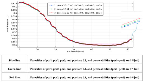
Figure 14.
Axial hydrogen mole-fraction profiles for combined sweeps of porosity (por1–por4 = 0.3, 0.4, 0.5) and permeability (per1–per4 = 10−10–10−12 m2); the red curve (ε = 0.5, k4 = 10−12 m2) yields the highest outlet.
A comparison of flow field/channel geometry strategies with an emphasis on hydrogen production consequences provides a one-stop summary of the results of this study alongside six previous benchmark references shown in Table 6. The first row (of this work) shows that grading the channel width w(x) to control residence time and reduce outlet velocity, without changing the overall flow direction or requiring manifold redesign, results in an increase in hydrogen production of 6.8%to 29%; at 1.3 V, the hydrogen output fraction is improved from H2 equal to 0.54 (Scenario S1: uniform channel) to 0.70 (Scenario S2: variable width channel) (+29%). The following rows summarize studies that rely on flow direction (co-current/counter-current/transverse), channel cross-section shape, or manifold design and report their implications on hydrogen production, mass/heat transfer behaviors, and operational constraints. As the Table 6 shows, the present approach achieves efficiency improvements by maintaining lateral temperature uniformity and slightly increasing pressure drop along the flow path. While many previous works have increased production at the cost of increasing thermal heterogeneity or hydraulic complexity, Table 6 thus provides a clear and level-headed comparison (as far as possible considering the differences in operating conditions of the references) between the current results and previous achievements.
Table 6.
Comparative Summary of SOEC Channel/Flow Designs and Hydrogen-Production Outcomes.
4. Conclusions
This study successfully designed, modeled, and evaluated a novel solid oxide electrolysis cell (SOEC) architecture featuring a variable channel width and an integrated heat transfer channel. Through high-fidelity computational fluid dynamics (CFD) analysis, five distinct geometric scenarios were investigated to optimize gas distribution, thermal management, and electrochemical performance. The key findings demonstrate that strategic modifications to the flow channel geometry profoundly impact the cell’s efficiency and hydrogen production rate. Specifically, Scenarios 2 and 4, which employed a systematically increasing channel width, yielded superior performance, enhancing hydrogen production by up to 29% compared to the base case at 1.3 V. This improvement is primarily attributed to a significantly reduced gas flow velocity and extended reactant residence time, which optimizes mass transport and reaction kinetics, rather than to changes in thermal distribution. The analysis of current density confirmed a strong positive correlation with operating voltage, with the maximum density reaching 7940 A/m2 at 1.3 V. Furthermore, the incorporation of a dedicated thermal channel was shown to improve heat dissipation, reduce ohmic losses, and promote a more uniform current distribution across the cell’s active area, particularly at lower voltages, where its impact is most dramatic. However, these performance enhancements are accompanied by increased system demands. The elevated hydrogen production and altered flow dynamics resulted in a higher internal cell pressure, a 7% increase in one scenario, which indicates an associated rise in the energy required for gas compression and circulation. In conclusion, this work validates that a variable-width channel design is a highly effective strategy for optimizing SOEC performance. By enhancing mass transport and current distribution while effectively managing thermal gradients, this design paves the way for more efficient and scalable high-temperature electrolysis systems. Future work should focus on experimental validation and optimizing the balance between performance gains and the associated energy consumption to maximize overall system efficiency.
These results have direct industrial applicability, as the “variable channel width” can be implemented with the same common technologies for fabricating SOEC interconnect plates—including stamping on Crofer-type ferritic steel, photochemistry/chemical etching for precise and gradual patterns, and machining/laser cutting for medium to high runs. The main advantage of this design is that only the channel width profile (w(x)) is changed without changing the materials, sealing, or manifold layout; thus, tooling costs and assembly risks remain low, while simulations show reduced local velocity, increased dwell time, and controllable pressure drop. In addition, manufacturing tolerances (±0.05–0.1 mm) are achievable with the aforementioned methods, and quality control can be performed by optical/3D measurements and leak testing. Conclusion: This design allows for optimization of mass transfer and gas feed uniformity with minimal changes to the current SOEC plate manufacturing chain and is therefore practical and economically feasible for large stack scales.
Raising the cell voltage from 1.4 to 1.5 V increases the hydrogen mole fraction across the channel in both operating scenarios, but the spatial response is configuration-dependent. Scenario 1 remains nearly uniform along the flow path—voltage primarily elevates the baseline composition with only a shallow axial gradient—whereas Scenario 2 exhibits a pronounced, monotonic enrichment toward the outlet, revealing stronger voltage sensitivity and improved through-plane/axial utilization. These results extend our lower-voltage trends (1.1–1.3 V) by showing that the qualitative ordering persists at higher drive, while Scenario 2 amplifies conversion gradients beneficial for overall yield.
Three-dimensional temperature fields remain smooth and laterally uniform, with a streamwise rise from inlet to outlet. For Scenario 2, the temperature range broadens from ~873–928 K at 1.4 V to ~872–997 K at 1.5 V, consistent with increased ohmic and reaction heating; however, no localized hot spots develop within the active area, indicating effective transverse heat spreading by the flow/geometry. A mesh-refinement study (≈5.74 × 10⁵ → 1.5 × 10⁶ cells) changed key observables by <1%, confirming mesh independence and lending confidence to all thermal and electrochemical fields reported.
Parametric sweeps show that increasing porosity in CGDL, CGDE, AGDE, and AGDL (por1–por4 → 0.5) systematically elevates the H2 mole fraction by reducing tortuosity and concentration polarization while lowering the outlet-side GDL permeability (per4 → 10−12 m2) further boosts outlet enrichment by limiting bypass, increasing residence time, and strengthening axial build-up.
Author Contributions
Conceptualization, M.M.A.; Methodology, M.M.A. and U.T.; Software, M.M.A.; Validation, M.M.A.; Investigation, U.T.; Resources, M.M.R.; Writing—original draft, M.M.A. and P.M.D.; Writing—review & editing, P.M.D.; Visualization, U.T. and M.M.R.; Supervision, U.T. and M.M.R.; Funding acquisition, P.M.D. All authors have read and agreed to the published version of the manuscript.
Funding
This research received no external funding.
Data Availability Statement
The original contributions presented in this study are included in the article. Further inquiries can be directed to the corresponding author.
Conflicts of Interest
The authors declare no conflict of interest.
Abbreviations
The following abbreviations are used in this manuscript:
| AK | Alkaline | ||
| CFD | Computational Fluid Dynamics | ||
| Cathode-GDL (CGDL) | Cathode Gas Diffusion Layer | ||
| Cathode-GDE (CGDE) | Cathode Gas Diffusion Electrode | ||
| Anode-GDL (AGDL) | Anode Gas Diffusion Layer | ||
| Anode-GDE (AGDE) | Anode Gas Diffusion Electrode | ||
| LSM | Lanthanum Strontium Manganite | ||
| PEM | Proton Exchange Membrane | ||
| SMR | Steam Methane Reforming | ||
| SOEC | Solid Oxide Electrolysis Cell | ||
| Symbols | |||
| ) | ) | ||
| ) | ) | ||
| ) | ) | ||
| ) | ) | ||
| ) | ) | ||
| ) | ) | ||
| ) | ) | ||
| ) | ) | ||
| ) | ) | ||
| ) | ) | ||
| ) | ) | ||
| ) | ) | ||
| ) | ) | ||
| ) | ) | ||
| ) | ) | ||
| ) | Mole fraction of species n | ||
| ) | Mass fraction of species m | ||
| Number of electrons transferred | ) | ||
| Greek symbols | |||
| Thermal expansion coefficient | Dynamic viscosity | ||
| Charge transfer coefficient (anode/cathode) | Poisson’s ratio | ||
| Inertial resistance coefficient in porous media | Electric potential | ||
| Kronecker delta | Density | ||
| Entropy change per reaction | Stress tensor | ||
| Porosity | Electrical conductivity | ||
| Total strain tensor | Tortuosity | ||
| Elastic strain | Solid volume fraction | ||
| Thermal strain | Frication coefficient | ||
| Over potential | |||
| Subscripts and superscripts | |||
| Anode | Species indices | ||
| cathode | Mass generation | ||
| Activation | Open circuit | ||
| Anode activation over potential | Ohimic over potential | ||
| Cathode activation over potential | Solid phase | ||
| Effective value | Layer or region indices | ||
| Electrolyte | Standard state | ||
| Gas system | Transpose | ||
References
- Francesco, S.; Alessandro, M.; Carlo, C.; Alessandro, B. Techno-economic analysis of wind-powered green hydrogen production to facilitate the decarbonization of hard-to-abate sectors: A case study on steelmaking. Appl. Energy 2023, 342, 121198. [Google Scholar] [CrossRef]
- Usman, M.R. Hydrogen storage methods: Review and current status. Renew. Sustain. Energy Rev. 2022, 167, 112743. [Google Scholar] [CrossRef]
- Boldrini, A.; Koolen, D.; Crijns-Graus, W.; van den Broek, M. The impact of decarbonising the iron and steel industry on European power and hydrogen systems. Appl. Energy 2024, 361, 122902. [Google Scholar] [CrossRef]
- Makki Abadi, M.; Rashidi, M.M. Machine Learning for the Optimization and Performance Prediction of Solid Oxide Electrolysis Cells: A Review. Processes 2025, 13, 875. [Google Scholar] [CrossRef]
- Aubras, F.; Deseure, J.; Kadjo, J.J.A. Two-dimensional model of low-pressure PEM electrolyser: Two-phase flow regime, electrochemical modelling and experimental validation. Int. J. Hydrogen Energy 2017, 42, 26203–26216. [Google Scholar] [CrossRef]
- Shangguan, Z.; Li, H.; Yang, B.; Zhao, Z.; Wang, T.; Jin, L.; Zhang, C. Optimization of alkaline electrolyzer operation in renewable energy power systems: A universal modeling approach for enhanced hydrogen production efficiency and cost-effectiveness. Int. J. Hydrogen Energy 2024, 49, 943–954. [Google Scholar] [CrossRef]
- Vo, N.D.; Oh, D.H.; Hong, S.-H.; Oh, M.; Lee, C.-H. Combined approach using mathematical modelling and artificial neural network for chemical industries: Steam methane reformer. Appl. Energy 2019, 255, 113809. [Google Scholar] [CrossRef]
- Nnabuife, S.G.; Darko, C.K.; Obiako, P.C.; Kuang, B.; Sun, X.; Jenkins, K. A comparative analysis of different hydrogen production methods and their environmental impact. Clean Technol. 2023, 5, 1344–1380. [Google Scholar] [CrossRef]
- Wendel, C.H.; Braun, R.J. Design and techno-economic analysis of high-efficiency reversible solid oxide cell systems for distributed energy storage. Appl. Energy 2016, 172, 118–131. [Google Scholar] [CrossRef]
- Jin, X.; Xue, X. Mathematical modeling analysis of regenerative solid oxide fuel cells in switching mode conditions. J. Power Sources 2010, 195, 6652–6658. [Google Scholar] [CrossRef]
- Zhang, B.; Harun, N.F.; Zhou, N.; Oryshchyn, D.; Colon-Rodriguez, J.J.; Shadle, L.; Bayham, S.; Tucker, D. A real-time distributed solid oxide electrolysis cell (SOEC) model for cyber-physical simulation. Appl. Energy 2025, 388, 125607. [Google Scholar] [CrossRef]
- Salihi, H.; Ju, H. Integrated modeling of electrochemical, thermal, and structural behavior in solid oxide electrolysis cells. Appl. Energy 2024, 353, 122041. [Google Scholar] [CrossRef]
- Xu, Y.; Chi, B.; Tu, Z. Performance evaluation and uniformity analysis of multi-stack solid oxide electrolysis cell (SOEC) systems under different arrangements. Int. J. Hydrogen Energy 2025, 173, 151339. [Google Scholar] [CrossRef]
- Wang, Y.; Du, Y.; Ni, M.; Zhan, R.; Du, Q.; Jiao, K. Three-dimensional modeling of flow field optimization for co-electrolysis solid oxide electrolysis cell. Appl. Therm. Eng. 2020, 172, 114959. [Google Scholar] [CrossRef]
- Der, O.; Olaitan, K.; Bertola, V. An experimental investigation of oil–water flow in a serpentine channel. Int. J. Multiph. Flow 2020, 129, 103327. [Google Scholar] [CrossRef]
- Kovalev, A.V.; Yagodnitsyna, A.A.; Bilsky, A.V. Plug flow of immiscible liquids with low viscosity ratio in serpentine microchannels. Chem. Eng. J. 2021, 417, 127933. [Google Scholar] [CrossRef]
- Virkar, A.V. Mechanism of oxygen electrode delamination in solid oxide electrolyzer cells. Int. J. Hydrogen Energy 2010, 35, 9527–9543. [Google Scholar] [CrossRef]
- Udagawa, J.; Aguiar, P.; Brandon, N.P. Hydrogen production through steam electrolysis: Model-based steady state performance of a cathode-supported intermediate temperature solid oxide electrolysis cell. J. Power Sources 2007, 166, 127–136. [Google Scholar] [CrossRef]
- Zeng, S.; Xu, M.; Parbey, J.; Yu, G.; Andersson, M.; Li, Q.; Li, B.; Li, T. Thermal stress analysis of a planar anode-supported solid oxide fuel cell: Effects of anode porosity. Int. J. Hydrogen Energy 2017, 42, 20239–20248. [Google Scholar] [CrossRef]
- Yang, P.; Feng, K.; Li, Z.-P. A review of advanced SOFCs and SOECs: Materials, innovative synthesis, functional mechanisms, and system integration. eScience 2025. advance online publication. [Google Scholar] [CrossRef]
- Jolaoso, L.A.; Bello, I.T.; Kazempoor, P. Operational and scaling-up barriers of SOEC and mitigation strategies to boost H2 production—A comprehensive review. Int. J. Hydrogen Energy 2023, 48, 31990–32013. [Google Scholar] [CrossRef]
- Sala, E.M.; Mazzanti, N.; Mogensen, M.B.; Chatzichristodoulou, C. Current understanding of ceria surfaces for CO2 reduction in SOECs and future prospects—A review. Solid State Ion. 2022, 375, 115833. [Google Scholar] [CrossRef]
- Ghamarinia, M.; Babaei, A.; Zamani, C.; Aslannejad, H. Application of the distribution of relaxation time method in electrochemical analysis of the air electrodes in the SOFC/SOEC devices: A review. Chem. Eng. J. Adv. 2023, 15, 100503. [Google Scholar] [CrossRef]
- Wang, Y.; Liu, Q.; Zhong, W. Techno-Economic analysis of coal and poultry manure combustion in a pressurized Oxy-Fuel CFB system coupled with SOEC. Appl. Therm. Eng. 2025, 279, 128107. [Google Scholar] [CrossRef]
- Lang, M.; Lee, Y.S.; Lee, I.S.; Szabo, P.; Hong, J.; Cho, J.; Costa, R. Analysis of electrochemical degradation phenomena of a 60-cell SOC stack operated in reversible SOFC/SOEC cycling mode. Appl. Energy 2025, 386, 125565. [Google Scholar] [CrossRef]
- Lahrichi, A.; El Issmaeli, Y.; Polle, B.G.; Ghrib, T. Advancements, strategies, and prospects of solid oxide electrolysis cells (SOECs): Towards enhanced performance and large-scale sustainable hydrogen production. J. Energy Chem. 2024, 94, 50–70. [Google Scholar] [CrossRef]
- Gholizadeh, T.; Abbaspour, N.; Ghiasirad, H.; Skorek-Osikowska, A. Sustainable biofuel production through anaerobic digestion, SOEC and carbon-capture-and-utilization (CCU): Techno-economic, exergy and Life-cycle analysis. Energy 2025, 317, 120894. [Google Scholar] [CrossRef]
- Liu, F.; Zhao, Z.; Xiao, L.; Zhou, R.; Liu, Q.; Ou, D.R.; Yuan, J. Multiphysics Analysis and Optimization of Solid Oxide Electrolysis Cells with Functionally Graded Fuel Electrodes. Thin-Walled Struct. 2025, 113936. [Google Scholar] [CrossRef]
- Zhu, H.; Zhu, J.; Zhu, P.; Xuan, J.; Ni, M.; Xu, H. Multi-objective optimization of SOEC performance in dynamic operation: A hybrid modelling approach towards thermal neutrality. Energy Convers. Manag. 2025, 337, 119926. [Google Scholar] [CrossRef]
- Liang, Z.; Chen, S.; Ni, M.; Wang, J.; Li, M. A novel control strategy to neutralize internal heat source within solid oxide electrolysis cell (SOEC) under variable solar power conditions. Appl. Energy 2024, 371, 123669. [Google Scholar] [CrossRef]
- Noren, D.A.; Hoffman, M.A. Clarifying the Butler–Volmer equation and related approximations for calculating activation losses in solid oxide fuel cell models. J. Power Sources 2005, 152, 175–181. [Google Scholar] [CrossRef]
- Liu, C.; Dang, Z.; Xi, G. Numerical study on thermal stress of solid oxide electrolyzer cell with various flow configurations. Appl. Energy 2024, 353, 122041. [Google Scholar] [CrossRef]
- Huang, M.; Jiang, H.; Liu, X.; Xiao, Y.; Kong, J.; Zhou, T. LSCM-GDC as composite cathodes for high temperature steam electrolysis: Performance optimization by composition and microstructure tailoring. Int. J. Hydrogen Energy 2022, 47, 34784–34793. [Google Scholar] [CrossRef]
- Momma, A.; Kato, T.; Kaga, Y.; Nagata, S. Polarization behavior of high temperature solid oxide electrolysis cells (SOEC). J. Ceram. Soc. Jpn. 1997, 105, 369–373. [Google Scholar] [CrossRef]
- Xu, Y.; Cai, S.; Chi, B.; Tu, Z. Numerical study on improved mass and heat transfer performance in a solid oxide electrolysis cell with sine wave flow field. Int. J. Hydrogen Energy 2025, 137, 806–818. [Google Scholar] [CrossRef]
- Wang, H.; Xiao, L.; Liu, Y.; Zhang, X.; Zhou, R.; Liu, F.; Yuan, J. Performance and thermal stress evaluation of full-scale SOEC stack using multi-physics modeling method. Energies 2023, 16, 7720. [Google Scholar] [CrossRef]
- Xu, Z.; Zhang, X.; Li, G.; Xiao, G.; Wang, J.Q. Comparative performance investigation of different gas flow configurations for a planar solid oxide electrolyzer cell. Int. J. Hydrogen Energy 2017, 42, 10785–10801. [Google Scholar] [CrossRef]
- Tu, Y.; Chai, J.; Li, S.; Han, F.; Zhang, Z.; Cai, W. The study of multiphysics field coupling and thermal stress in three types of Solid Oxide Electrolysis Cells (SOEC). Int. J. Electrochem. Sci. 2024, 19, 100789. [Google Scholar] [CrossRef]
- Ryu, D.; Lim, J.; Lee, W.; Hong, J. Contactless external manifold design of a kW-scale solid oxide electrolysis cell stack and analysis of its impact on the internal stack environment. Energy Convers. Manag. X 2025, 26, 100934. [Google Scholar] [CrossRef]


Disclaimer/Publisher’s Note: The statements, opinions and data contained in all publications are solely those of the individual author(s) and contributor(s) and not of MDPI and/or the editor(s). MDPI and/or the editor(s) disclaim responsibility for any injury to people or property resulting from any ideas, methods, instructions or products referred to in the content. |
© 2025 by the authors. Licensee MDPI, Basel, Switzerland. This article is an open access article distributed under the terms and conditions of the Creative Commons Attribution (CC BY) license (https://creativecommons.org/licenses/by/4.0/).