Article

Predicting the Remaining Service Life of Power Transformers Using Machine Learning

1
School of Electronics and Information Engineering, Liaoning Technical University, Huludao 125105, China
2
School of Software, Liaoning Technical University, Huludao 125105, China
3
School of Electrical and Control Engineering, Liaoning University of Engineering and Technology, Huludao 125105, China
4
Business School, Shanghai Jianqiao University, Shanghai 200125, China
*
Author to whom correspondence should be addressed.
Processes 2025, 13(11), 3459; https://doi.org/10.3390/pr13113459
Submission received: 17 September 2025 / Revised: 8 October 2025 / Accepted: 20 October 2025 / Published: 28 October 2025
(This article belongs to the Section Energy Systems)

Abstract

In response to the insufficient adaptability of power transformer remaining useful life (RUL) prediction under complex working conditions and the difficulty of multi-scale feature fusion, this study proposes an industrial time series prediction model based on the parallel Transformer–BiGRU–GlobalAttention model. The parallel Transformer encoder captures long-range temporal dependencies, the BiGRU network enhances local sequence associations through bidirectional modeling, the global attention mechanism dynamically weights key temporal features, and cross-attention achieves spatiotemporal feature interaction and fusion. Experiments were conducted based on the public ETT transformer temperature dataset, employing sliding window and piecewise linear label processing techniques, with MAE, MSE, and RMSE as evaluation metrics. The results show that the model achieved excellent predictive performance on the test set, with an MSE of 0.078, MAE of 0.233, and RMSE of 11.13. Compared with traditional LSTM, CNN-BiGRU-Attention, and other methods, the model achieved improvements of 17.2%, 6.0%, and 8.9%, respectively. Ablation experiments verified that the global attention mechanism rationalizes the feature contribution distribution, with the core temporal feature OT having a contribution rate of 0.41. Multiple experiments demonstrated that this method has higher precision compared with other methods.

1. Introduction

Constructing a new type of power system is the core foundation for implementing the new energy security strategy and a key carrier for achieving the “dual carbon” goals. As the core equipment of the power system, the remaining useful life (RUL) prediction capability of power transformers has become a strategic focus for ensuring reliable system operation [1]. Prognostics and health management (PHM) is an intelligent technology system that monitors equipment status in real time, predicts potential failures, and optimizes maintenance strategies. It aims to upgrade traditional reactive maintenance to proactive assurance. Its core functions include condition monitoring, fault diagnosis, health prediction, and decision support, which are widely applied in aerospace, industrial manufacturing, and energy power sectors. PHM significantly reduces maintenance costs and enhances system reliability. Remaining useful life (RUL) prediction technology is a core research direction in the field of prognostics and health management, integrating multidisciplinary theories and methods. Its technical foundation covers sensor networks, big data analytics, physical modeling, and machine learning algorithms, and it is evolving towards edge computing and multimodal fusion for more precise RUL prediction. Accurate RUL prediction technology, by integrating state perception data with intelligent assessment models, not only provides a scientific basis for equipment condition-based maintenance but also optimizes asset lifecycle management. It is indispensable technical support for building a new type of power system, directly affecting the energy transition process and the path to achieving the “dual carbon” goals [2]. Currently, RUL prediction technology is divided into two main categories: data-driven methods and physical model-based methods. Data-driven methods are the mainstream technology for RUL prediction, focusing on mining the performance degradation patterns of equipment from historical data. Physical models describe the degradation process based on the working principles and failure mechanisms of the equipment, using mathematical formulas such as the Paris crack growth model and the Arrhenius equation [3].
The development of industrial IoT and intelligent sensing technologies has accelerated the adoption of machine learning in intelligent fault diagnosis. For industrial time series forecasting, scholars increasingly utilize machine learning methods due to their exceptional scalability and accuracy. Deep learning excels at handling high-dimensional complex data, such as images, speech, and time series, through its multi-layer nonlinear feature extraction and end-to-end learning capabilities. It achieves superior accuracy and generalization in perception, prediction, and decision-making tasks compared to traditional models. Wu Shimiao et al. [4] proposed a residual life prediction model based on a multi-scale CNN with skip connections, which achieved high-precision life prediction by integrating local and global feature information across different scales. However, this approach faces the risk of CNN’s sensitivity to input size and the potential neglect of global trends in the degradation process during local feature extraction.
In industrial time series prediction, the limitations of single-network models result in poor generalization for complex industrial data, susceptibility to data distribution shifts and concept drift, and difficulty in capturing both local fluctuations and long-term trends in time series data simultaneously. In recent years, Transformer has gained popularity in industrial time series prediction due to its global modeling capability of self-attention mechanisms, parallel computing efficiency, and strong representation of multivariate nonlinear time series features. Xu Tao et al. [5] utilized the self-attention mechanism of Transformer to efficiently model dynamic features and noise patterns in industrial sensor time series data, significantly improving feature distinguishability in blind denoising tasks without requiring clean data. Their network expanded the receptive field through dilated convolution and alleviated gradient degradation with residual connections, outperforming traditional CNNs, LSTM models, and pure autoencoder methods. As technology advances, attention mechanisms have been increasingly highlighted for their ability to dynamically allocate weights to different time steps in a sequence, flexibly capturing long- and short-term dependencies and significantly enhancing the accuracy of time series prediction. They are particularly adept at handling variable-length inputs and non-stationary patterns while supporting parallel computing acceleration.
Despite extensive research by scholars, the following limitations persist: (1) Traditional recurrent neural networks struggle to effectively capture long-term dependencies within sequences. (2) Training and inference speeds for complex models are slow, with high computational costs. (3) Unidirectional recurrent neural networks cannot utilize future contextual information to model the current state. (4) Models treat all time steps or features equally when processing sequences, failing to distinguish their importance and causing critical information to be obscured. (5) Insufficient spatiotemporal feature fusion prevents simultaneous and effective consideration of interactions between temporal and spatial dimensions. (6) Models exhibit inadequate feature extraction capabilities and predictive accuracy.
To address the aforementioned challenges, this study proposes a network architecture based on a parallel Transformer–BiGRU–GlobalAttention framework. Initially, the Transformer’s strengths are harnessed to extract long-term temporal dependencies within the sequence, while a parallel structure is employed to accelerate the model’s training and inference processes, thereby enhancing the model’s ability to perceive critical information. Subsequently, the characteristics of the bidirectional gated recurrent unit (BiGRU) are utilized to model the sequence bidirectionally, from both forward and backward directions, which allows for a more effective capture of dependencies within the sequence. The GlobalAttention mechanism is then applied to weight the outputs of the BiGRU, enabling the model to focus more efficiently and swiftly on the most salient spatial features within the sequence, thereby significantly improving predictive performance. Additionally, the cross-attention mechanism is employed to integrate spatiotemporal features from the parallel network, achieving a simultaneous consideration of temporal and spatial relationships. This approach enables the model to better capture features within spatiotemporal sequence data, effectively enhancing the representation of features and realizing high-precision feature extraction and predictive performance.

2. Theoretical Foundations

2.1. Transformer

The Transformer is a revolutionary model introduced by Vaswani et al. in 2017. Its core innovation lies in the complete reliance on the self-attention mechanism to replace traditional recurrent neural networks (RNNs) and convolutional neural networks (CNNs), thereby addressing the issues of long-range dependencies and parallel computing bottlenecks in sequence modeling. Originally designed to provide a more efficient architecture for machine translation tasks, it quickly became a cornerstone in the field of natural language processing (NLP) and even multimodal domains [6]. The self-attention mechanism dynamically computes the association weights of each position in the sequence, enabling the model to focus on key information. Specifically, the input vectors are mapped to three matrices: Query (Q), Key (K), and Value (V). The attention scores are calculated through scaled dot-product operations:
A t t e n t i o n Q , K , V = s o f t m a x Q K T d k V
In this formulation, d k serves as the scaling factor, where d k denotes the dimensionality of the key vector. This scaling factor is specifically designed to counteract the numerical inflation that occurs after the dot-product operation, thereby stabilizing the gradient values. The multi-head attention mechanism further enhances the model’s ability to capture complex relationships by parallelizing multiple self-attention subspaces. Moreover, Positional Encoding is introduced into the input, injecting sequence position information through sine/cosine functions or learnable parameters, thus compensating for the lack of sequential perception inherent in non-recurrent architectures.
As depicted in Figure 1, the Transformer architecture employs an encoder–decoder structure, with both the encoder and decoder comprising multiple stacked layers of identical configuration. The encoder consists of self-attention layers and feed-forward networks (FFN), while the decoder additionally incorporates encoder–decoder attention layers to cross-attend to the encoder’s output. Each layer utilizes residual connections and layer normalization to mitigate the vanishing gradient problem. This design not only stabilizes the training of deep models but also supports parallel computation, thereby significantly enhancing efficiency.

2.2. BiGRU-GlobalAttention

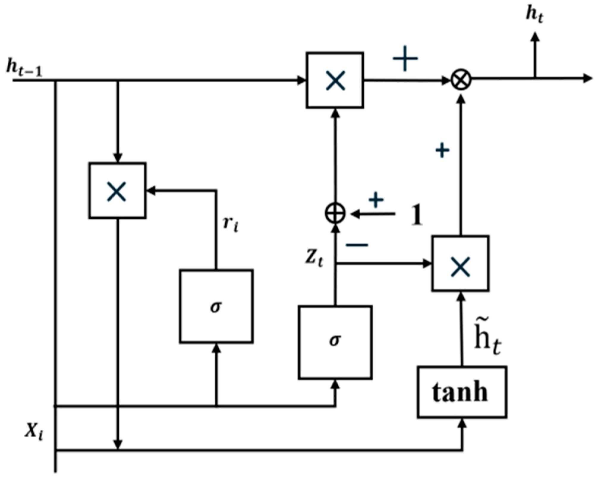
The gated recurrent unit (GRU), proposed by Cho et al. in 2014, aims to address the challenges of modeling long-range dependencies in traditional recurrent neural networks (RNNs) due to gradient vanishing or exploding [7], while also simplifying the complex gating structure of long short-term memory (LSTM). By integrating the forget and input mechanisms, GRU reduces the number of parameters, thereby enhancing computational efficiency while maintaining performance, and has rapidly become one of the mainstream architectures for sequence modeling. The core of the GRU lies in the introduction of the update gate and the reset gate, which dynamically control the retention and forgetting of information. Specifically, given the current input x t and the previous hidden state h t 1 , the two gates are computed using the following formulas:
z t = σ ( W z · h t 1 , x t + b z )           ( Update   Gate )
r t = σ W r · h t 1 , x t + b r           ( Reset   Gate )
In this context, σ represents the Sigmoid activation function, and W z , W r and b z , b r are the learnable parameters. The update gate determines the retention ratio of the preceding state h t 1 , while the reset gate modulates the correlation between historical information and the current input. Subsequently, the candidate state h t t i l d e is generated based on the reset gate-adjusted historical information and the current input.
h t t i l d e = t a n h W h r t h t 1 , x t + b h
Ultimately, the current hidden state h t is obtained using the update gate through a weighted fusion of the previous state and the candidate state.
h t = 1 z t h t 1 + z t h t t i l d e
As illustrated in Figure 2, compared with the LSTM, the GRU omits the output gate and cell state, achieving a lightweight structure through its two-gate mechanism, albeit at the cost of sacrificing some fine-grained control over long-term memory. Owing to its low computational cost and high parallelizability, the GRU has been widely applied in natural language processing, speech recognition, and time series prediction [8]. It has particularly excelled in scenarios with limited resources. Although the LSTM still holds an edge in complex tasks, the GRU, with its simplicity and efficiency, remains an important baseline model for sequence modeling [9].
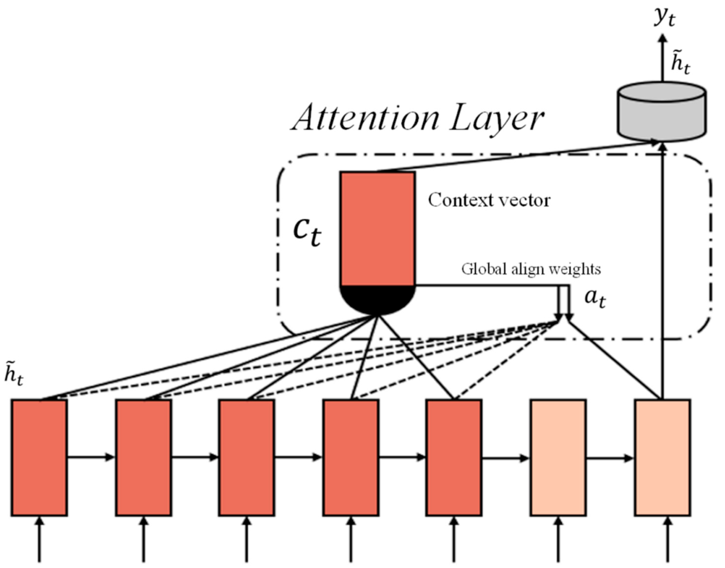
The early implementation of global attention is closely related to the RNN architecture [10]. Its global perception characteristics serve as the theoretical foundation for sparse attention mechanisms (such as Longformer) and linearized attention mechanisms (such as Linformer), and it represents a milestone in sequence-to-sequence models. Global attention is an attention mechanism that dynamically computes the association weights between all elements in the input sequence and the target position. Its core lies in capturing long-range dependencies and breaking through the limitations of local vision [11]. Unlike traditional local attention, global attention allows the model to equally focus on all positions of the entire input sequence when processing a particular position. It is especially suitable for tasks where there is a significant difference in length between the input and output or where global context is required [12].
Here, h i denotes the hidden state of the decoder at the target position i, s j represents the hidden state of the encoder at the input position j, q i is the query vector derived from h i , and k j is the key vector derived from s j . The core formula of global attention is typically based on the interaction of Query, Key, and Value [13]. Taking additive attention as an example [14], given the decoder’s hidden state h i at target position i and the encoder’s hidden state s j at input position j, the attention weight α i j is computed as follows:
α i j = e x p e i j k = 1 N e x p e i k ,           e i j = v T t a n h W 1 h i + W 2 s j
In this formulation, W 1 , W 2 are learnable parameters, and v is a weight vector. By contrast, the scaled dot-product attention mechanism streamlines the computation process as follows:
α i j = e x p q i k j / d k k = 1 N e x p q i k k / d k
Herein, q i denotes the query vector, and k j represents the key vector. The Transformer model further employs multi-head attention, executing multiple linear transformations in parallel to enhance the representation capability.
As illustrated in Figure 3 and Figure 4, we have improved the GRU based on the attention mechanism to a BiGRU based on the global attention mechanism. By integrating bidirectional gated recurrent units with the global attention mechanism and employing a global attention model, we first generate dynamic weight scores for each time step using a scoring function. Subsequently, based on the soft attention mechanism, we calculate the weight scalar values for each time step. We then perform an element-wise multiplication between the weight vectors and the corresponding hidden states to generate context vectors β(i) with global perception. Finally, we aggregate and sum the weighted vectors of all time steps to output the hidden state representation that integrates global dependencies. The BiGRU network optimized by global attention can better capture the key information in sequence data, thereby enhancing the performance and effectiveness of the model.

2.3. Cross-Attention Feature Fusion

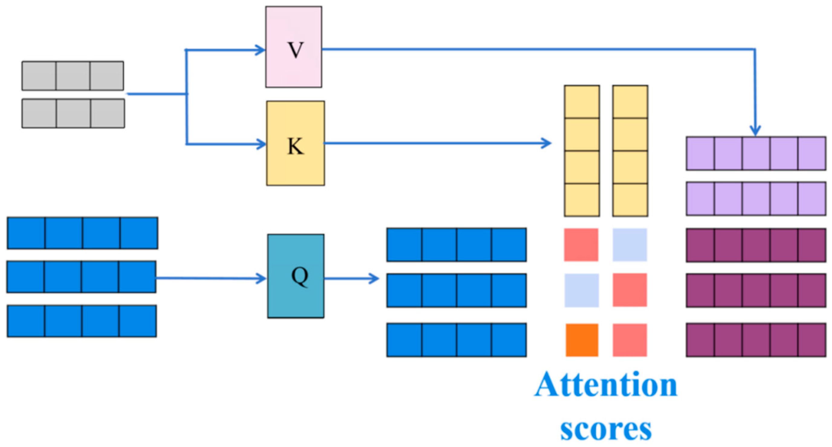
The cross-attention mechanism is a core technique in deep learning for modeling dependencies between two heterogeneous sequences [15]. Its essence lies in facilitating cross-sequence information interaction through dynamic weight allocation. Unlike self-attention mechanisms, which focus solely on internal relationships within the same sequence [16], cross-attention involves queries (Query) and key–value pairs (Key–Value) from different sequences. For instance, in machine translation, the decoder’s query corresponds to the target language sequence, while the encoder’s key–value pairs correspond to the source language sequence. As depicted in Figure 5, the core computational process can be formalized as follows [17]:
A t t e n t i o n Q , K , V = s o f t m a x Q K T d k V
In this context, Q R L q × d q represents the query matrix, while K R L k × d k and V R L k × d v denote the key and value matrices, respectively. Here, L q and L k correspond to the lengths of the respective sequences, and d k and d v signify the dimensions of the feature space. The product Q K T computes the similarity matrix between queries and keys. The term d k serves as a scaling factor to mitigate the risk of vanishing gradients in the Softmax function due to large inner products. The Softmax function subsequently normalizes these similarities into a probabilistic distribution. The final output is derived through a weighted summation over the matrix V . The interpretability of this mechanism is encapsulated in the attention weights A = s o f t m a x Q K T / d k , where each element A i j quantifies the dependency strength of the i -th position in the query sequence on the j -th position in the key sequence.

2.4. Parallel Transformer–GlobalAttention–BiGRU Model

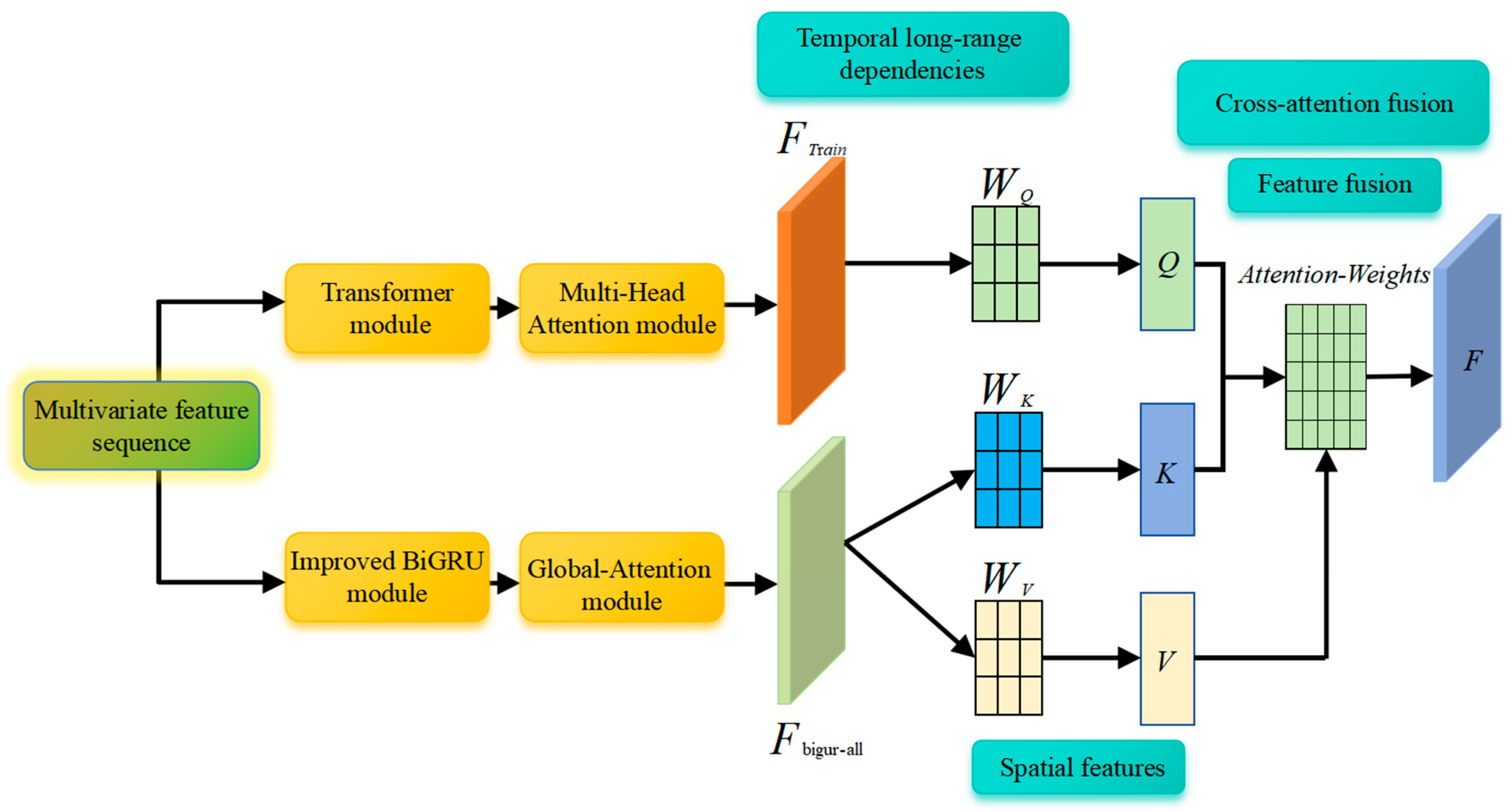
The architecture of the proposed parallel Transformer–BiGRU–GlobalAttention model is illustrated in Figure 6. multivariate time series data initially undergo the Transformer encoder layer, which is predicated on the multi-head attention mechanism, to distill features associated with long-term dependencies [18]. Concurrently, the data are processed through the BiGRU network, which is optimized by GlobalAttention, to extract global spatial features. Subsequently, the cross-attention mechanism is employed to amalgamate these features by calculating attention weights, thereby enabling the model to accentuate salient features. This is succeeded by an enhanced feature fusion step, culminating in high-precision prediction via a fully connected layer. To elaborate, the model is bifurcated into two parallel branches for feature extraction [19].
Branch 1 employs a Transformer encoder layer model predicated on the multi-head attention mechanism. The Transformer, a sequence modeling approach founded on the self-attention mechanism, models dependencies between distinct positions within a sequence and is capable of capturing global contextual information [20].
In Branch 2, multivariate sequence data are simultaneously processed through the BiGRU network (Implemented based on Python 3.8 and PyTorch 1.12.1 framework, where the GlobalAttention mechanism is built using PyTorch’s custom module functionality) optimized by GlobalAttention. GlobalAttention is a mechanism designed to enhance the model’s focus on different parts of the input sequence. Within the BiGRU model, the global attention mechanism assists the model in concentrating on the most relevant portions of the input sequence, thereby improving performance and generalization capability. At each time step, the global attention mechanism computes a weight vector that represents the model’s focus on various parts of the input sequence. These weights are then applied to the feature representations output by the BiGRU, weighting the features across all positions [21]. This allows the model to selectively focus on important global spatial features, thereby augmenting its perception of spatial features in multivariate sequences. The model employs a parallel prediction structure, enabling simultaneous prediction of multiple time steps. This parallel prediction mechanism accelerates training and inference while fully leveraging the information contained in time series data to enhance prediction performance. The cross-attention mechanism fuses spatial and temporal features by calculating attention weights, learning correlations between different positions in spatiotemporal features. This enables the model to better capture features in spatiotemporal sequence data, thereby enhancing model performance and generalization ability [22].

3. Experimental Design

3.1. Data Source

In the experiments, the model training and testing operations were conducted using PyCharm (Python 3.9 and PyTorch 1.8 or above versions are all compatible), with the experimental environment based on PyTorch 3.0.1. All programs were executed on a computer with the following configuration: Windows 11 (Microsoft in Redmond, WA, USA), 13th Gen Intel(R) Core(TM) i7-13620H, NVIDIA GeForce RTX 4060 Laptop GPU (NVIDIA in Santa Clara, CA, USA), and 8 GB RAM.
The proposed remaining useful life (RUL) prediction model was evaluated using the widely recognized Electricity Transformer Temperature (ETT) dataset. This dataset comprises multiple sub-datasets, namely ETTh1, ETTh2, ETTm1, and ETTm2. The ETTh1 and ETTh2 datasets record transformer feature data at hourly intervals, while ETTm1 records data at 15 min intervals and ETTm2 at 1 min intervals, as detailed in the reference. For experimental validation, the ETTh2 sub-dataset was selected. This sub-dataset is specifically designed for high-frequency monitoring scenarios and contains dense sensor sampling data. The training set includes continuous high-frequency time series data of power transformers, ranging from normal operation to potential failure states. It records dynamic parameters such as the oil temperature of the bushing, winding temperature of the core, main transformer load current, and ambient temperature and humidity, covering typical daily load fluctuations and seasonal environmental changes. The test set comprises real-time monitoring data and corresponding RUL labels in the 12 to 24 h preceding the occurrence of a fault, which are used for the model’s short-term temperature trend extrapolation and life endpoint prediction. It should be noted that the operational data from Beijing Guowang Fuda Technology Development Co., Ltd. (Beijing, China), mentioned in Section 3.2, were used for data visualization, feature description, and auxiliary verification of the model’s effectiveness; all experimental results reported in this study are based on the public ETTh2 dataset.

3.2. Data Preprocessing

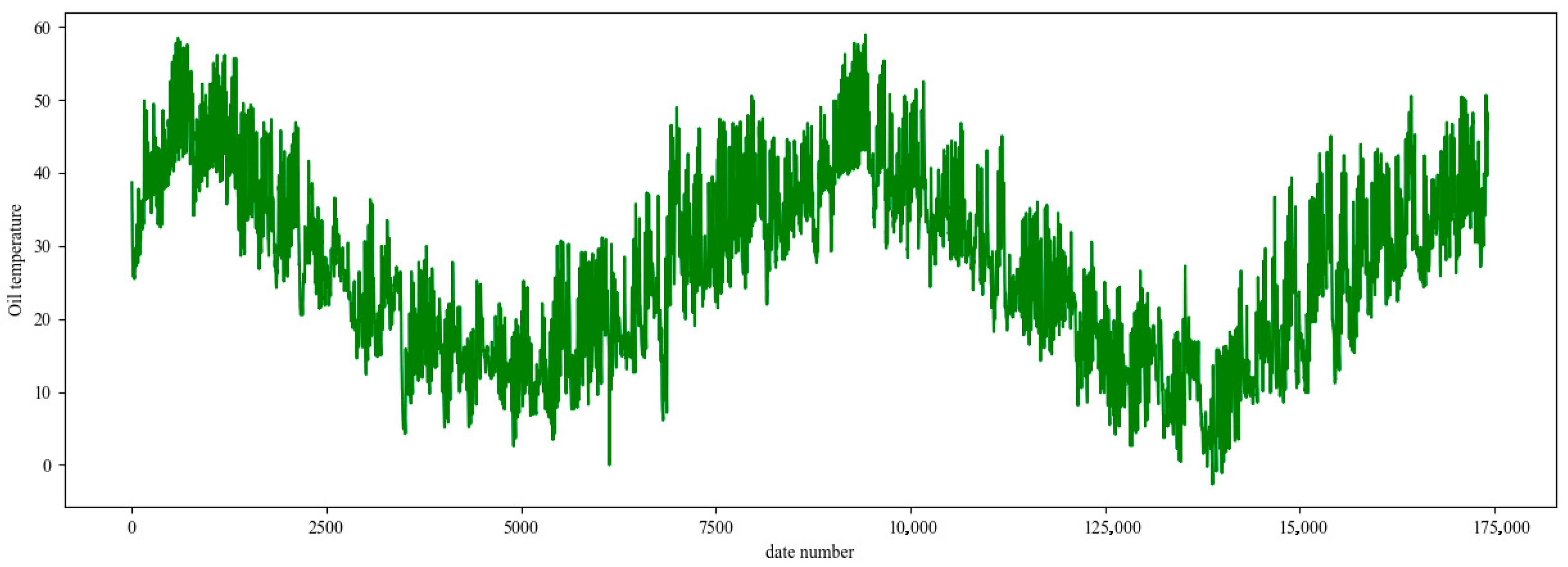
The oil temperature data are incorporated into the scope of this study, as depicted in Figure 7, which highlights the intrinsic nature of the power distribution problem. Power grids are required to manage power distribution dynamically in accordance with the fluctuating demands of consumers. However, the prediction of electricity demand in specific regions is significantly complex, being influenced by a multitude of factors such as weekday/holiday patterns, seasonal changes, weather variations, and ambient temperature. Existing forecasting methods struggle to maintain high accuracy in long-term real-world scenarios, and forecasting errors can lead to severe consequences such as overloading of power grid equipment or insufficient supply. This technical bottleneck compels managers to resort to empirical threshold methods for decision-making. However, these empirical values are typically set conservatively, resulting in excessive consumption of power resources and accelerated depreciation of equipment.
As shown in Table 1 and Table 2, it is worth noting that the oil temperature data of power transformers hold significant monitoring value. Serving as a core parameter reflecting the operational condition of transformers, oil temperature data can indirectly characterize the load status of the equipment. By accurately predicting the trends in transformer oil temperature changes and constructing a load capacity assessment model, it is possible to optimize power distribution strategies while ensuring the safe operation of the equipment. In this study, real operational data over a two-year period, provided by Beijing Guowang Fuda Technology Development Company, were utilized. The modified dataset not only includes the time series data of oil temperature but also encompasses load parameters and environmental variables corresponding to the respective time periods, thereby providing a reliable basis for establishing a dynamic load capacity assessment model.
(1) Data Normalization
This research constructs a remaining useful life (RUL) prediction dataset through a multi-stage data processing procedure, the core workflow of which is as follows: In the data preprocessing stage, the Z-score standardization method is employed to conduct zero-mean normalization on seven sensor features (including HUFL, HULL, MUFL, etc.) and the target variable OT, scaling the data of each sensor channel to the range [0, 1]. The normalization formula is as follows:
x ~ s = x s μ s σ s
In the formula, μ s and σ s represent the sample mean and standard deviation of the data in each sensor channel, respectively. x s denotes the original measurement value of sensor channel s, while x ~ s represents the normalized measurement value of sensor channel s. Here, μ s is the sample mean of the data in sensor channel s, and σ s is the sample standard deviation of the data in sensor channel s.
(2) Sliding window processing
Sliding window processing is a widely used feature extraction method for time series data. For the entire cycle of an engine from operation to failure, assuming the total number of operating cycles of the engine is T , we define the sliding window size as W and the sliding step as S . Under this setting, each sample contains data from W consecutive time steps, with each time step comprising N feature dimensions. In the code implementation, the data form of each sample is a W × N matrix, where N represents the number of features. For the i + 1-th sample, the corresponding remaining useful life (RUL) calculation formula is as follows:
R U L i = T W i × S
In the above formula, R U L i denotes the predicted remaining useful life corresponding to the i-th window, T is the total number of operating cycles of the engine, and W is the size of the sliding window. In this study, W is chosen to be 12 to ensure sufficient temporal information. i is the sample index, and S is the sliding step, which is selected to be 1 in this study to retain the maximum amount of information. It should be noted in the data partitioning process that the window size must not exceed the minimum number of cycles in the training and testing sets; otherwise, it may lead to data truncation or information loss. Through multiple experiments, this study has verified that the chosen window size W = 12 can ensure that the model learns long-term temporal dependencies while maximizing the number of samples and avoiding data redundancy.
(3) RUL Label Processing
To effectively enhance the prediction accuracy of industrial equipment operational reliability, this study employs a piecewise linear processing method for the labels. In this field, piecewise linear functions are commonly used to generate labels. This approach sets appropriate degradation thresholds, and once the health status of a power transformer falls below the degradation threshold, its health status linearly deteriorates with the increase in operating cycles until a severe defect occurs. Similar to previous studies, the abnormality threshold in this study is set at 125, meaning that when the prediction error is less than 125, it is determined to be a normal operating state. This abnormality processing method can effectively reduce the interference of outliers on the prediction model while avoiding an excessive focus on normal fluctuations during the stable phase [23]. Additionally, constraining model behavior reduces the risk of extreme value interference and prevents the algorithm from overfitting to the characteristics of the health status data.
(4) Evaluation Metrics
The mean absolute error (MAE) is defined as the average of the absolute differences between the predicted values and the true values. It assigns equal weight to all errors. The formula is as follows:
M A E = 1 n i = 1 n y i y ^ i
In the above formula, n represents the number of samples, y i is the true value of the i-th sample, and y ^ i is the predicted value of the i-th sample. The unit of MAE is consistent with that of the original data, and it is relatively insensitive to outliers. A smaller value of MAE indicates better model prediction performance.
The mean squared error (MSE) is defined as the average of the squared differences between the predicted values and the true values. It imposes a higher penalty for larger errors. The formula is as follows:
M S E = 1 n i = 1 n y i y ^ i 2
It shares the same characteristics as MAE, but its unit is the square of the original data error. It assigns greater weight to outliers. A smaller value indicates better model prediction performance.
The root mean squared error (RMSE) is defined as the square root of the MSE. It restores the unit of MSE to the same unit as the original data, making the error more interpretable. The formula is as follows:
R M S E = 1 n i = 1 n y i y ^ i 2 = M S E
It is the square root of the MSE and has the same unit as the original data. It takes into account the magnitude of the errors and amplifies the impact of larger errors. A smaller value indicates better model prediction performance. Note: The reported MAE, MSE, and RMSE values in the results sections are calculated on the original scale of the target variable (OT in °C) after inverse transformation, to provide interpretable error metrics in the actual physical unit.
The mean absolute percentage error (MAPE) is employed to quantify the average magnitude of the relative prediction errors, providing an intuitive assessment of the model’s accuracy in percentage terms. It is calculated as follows:
MAPE = 100 % n i = 1 n y i y ^ i y i
where y i is the actual value, y ^ i is the predicted value, and n is the total number of samples. This metric effectively normalizes the absolute error by the actual value, making it particularly useful for understanding the proportional error across datasets with different scales. A lower MAPE value indicates higher predictive precision of the model.
The coefficient of determination, denoted as R2, is utilized to evaluate the goodness-of-fit of the model by measuring the proportion of the variance in the dependent variable that is predictable from the independent variables. Its calculation is defined by the following formula:
R 2 = 1 i = 1 n y i y ^ i 2 i = 1 n y i y 2
In this expression, y represents the mean of the actual observations. The numerator quantifies the total squared errors of the predictions, while the denominator represents the total variance within the actual data. An R2 value close to 1 signifies that the model explains a large portion of the data variance, indicating excellent explanatory power.

3.3. Model Parameter Settings

The specific parameters and hyperparameter settings for each module in the model are shown in Table 3. In the model training phase of this study, the robust Adam optimizer was employed for parameter optimization. This optimizer can automatically adjust the learning rate based on the gradient changes, effectively accelerating the model’s convergence speed in the early stages of training. To thoroughly analyze the model’s performance under different conditions, various combinations of learning rates and batch sizes were tested in the experiments. The initial learning rate was ultimately set to 0.003, which ensured that the learning process maintained numerical stability while guaranteeing convergence efficiency.
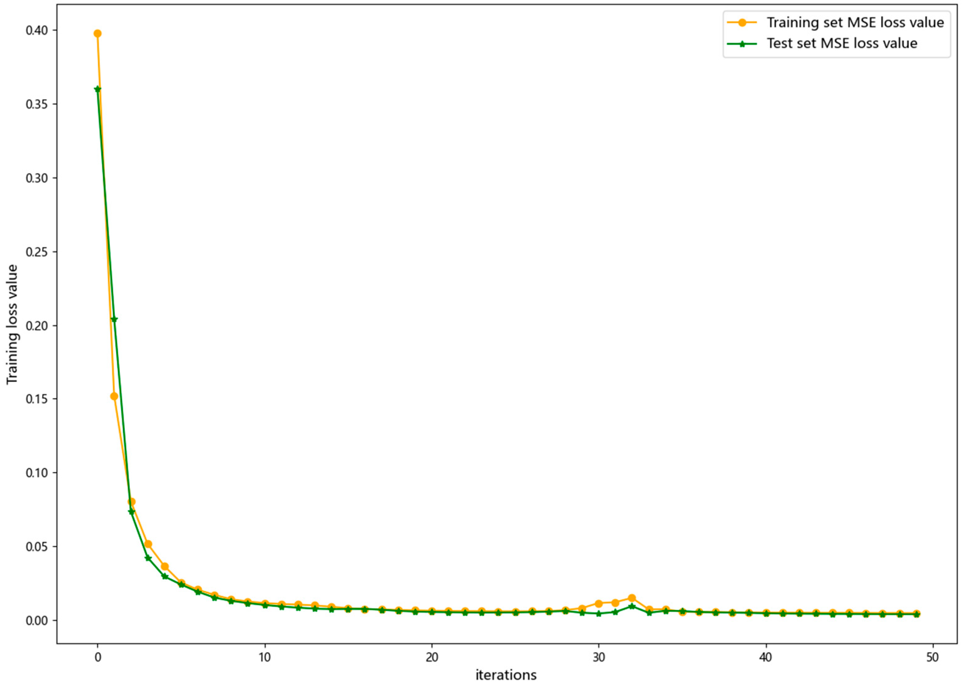
To alleviate overfitting and enhance the model’s generalization capability, this study utilized a combination of the EarlyStop strategy and regularization techniques. These two approaches worked synergistically to effectively improve the model’s adaptability to unseen data. The model’s hyperparameter configuration in this study was determined through multiple systematic experiments. After several rounds of parameter combination comparisons and performance evaluations, the model demonstrated the best predictive performance on the ETT dataset. It is important to note that the loss values (MSE_Loss) shown in Figure 8 are computed on the normalized dataset during the training phase. Therefore, the final training loss of approximately 0.005 is a dimensionless value. In contrast, the performance metrics (e.g., MSE, RMSE) reported in the result tables (Section 4) are calculated on the original physical scale (°C) after inverse transformation of the model’s predictions. This explains the apparent discrepancy in numerical values.

4. Experimental Results

After training the parallel Transformer–BiGRU–GlobalAttention model with hyperparameters, the algorithm model was tested and verified using training and testing datasets. As shown in Figure 8, the model exhibited rapid loss reduction in the initial phase (approximately the first 5 iterations), quickly dropping from a high initial value between 0.35 and 0.4 to a lower level of about 0.05. It then entered a gradual decline phase, where the loss continued to decrease but at a significantly slower rate between approximately 15 and 30 iterations, eventually stabilizing at a very low level of about 0.005. The loss curves for the training and testing sets are highly consistent, indicating that the model not only learns quickly but also has good generalization ability without severe overfitting. After about 30 iterations, both curves tend to stabilize, indicating that the model has essentially converged, and continuing to increase the number of iterations may not bring significant performance improvements.
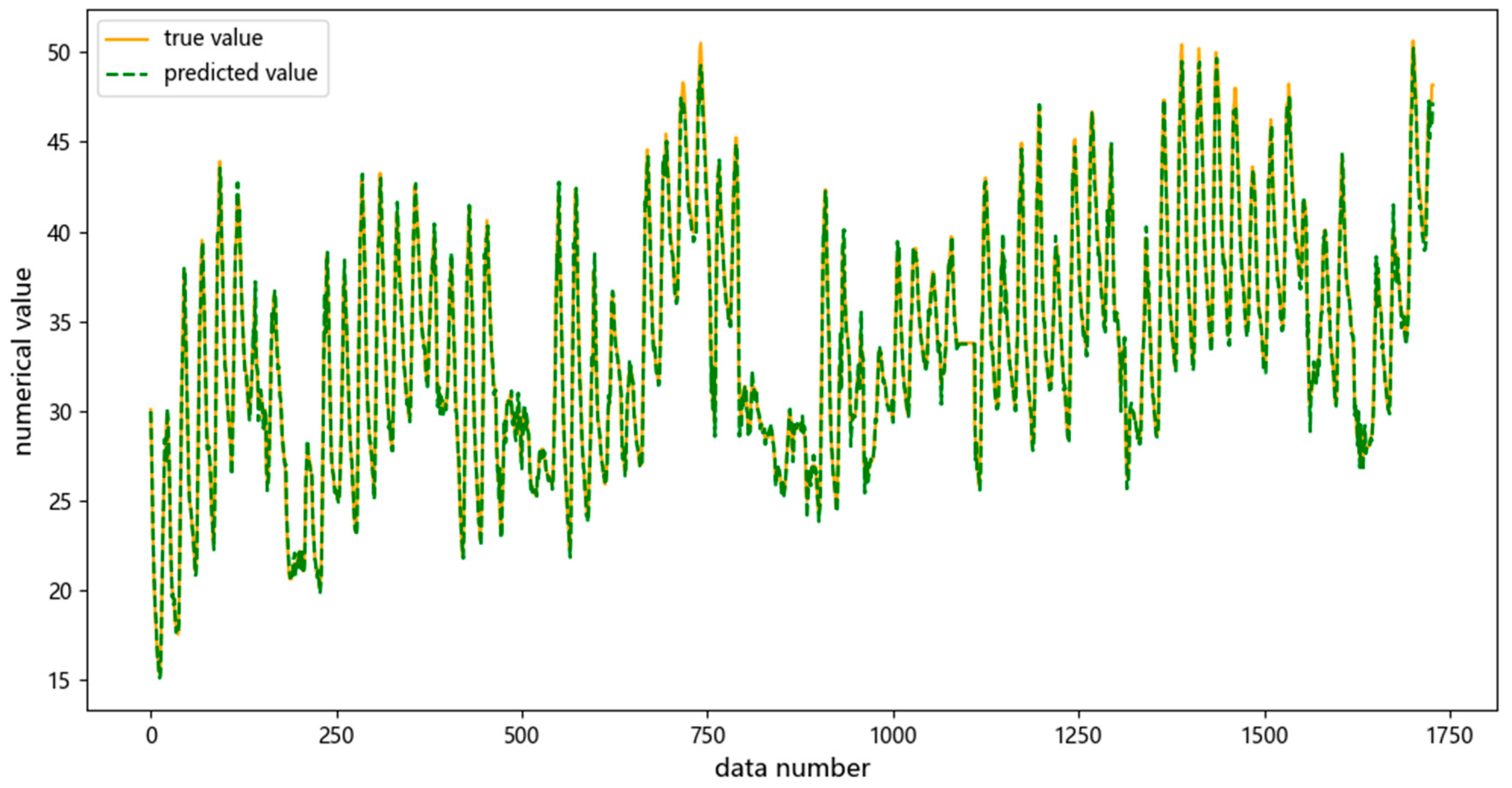
According to Figure 9, the comparative analysis of the prediction results for the test set’s time series data is shown, with the dashed line representing the predicted values and the solid line representing the true values. It can be observed that the two have similar degradation trajectories. Several key characteristics can be noted from the figure: The overall fit is relatively high, indicating that the model has a high level of predictive accuracy. Across the entire time span (0–1750), the trends of the two sequences are highly consistent. The data exhibit frequent fluctuations, mainly concentrated in the range of 25–50, and the model successfully captures these subtle changes and fluctuation patterns. At several key time points (such as near 500, 750, 1000, and 1500), the predicted values are almost identical to the true values, demonstrating the model’s excellent performance in handling extreme points and turning points. The prediction error is minimal, showing a high level of prediction accuracy. Overall, the model demonstrates excellent time series forecasting capabilities and can be used to support related decision-making or predictive tasks.
To fully demonstrate the superiority of the method proposed in this paper, the Transformer–GlobalAttention–BiGRU model is compared with other currently publicly available predictive models. The experimental comparison results are shown in Table 4. According to the data analysis in the table, the Transformer–GlobalAttention–BiGRU model proposed in this paper significantly outperforms other comparison methods in terms of predictive performance. Its mean squared error (MSE) is as low as 0.078, the mean absolute error (MAE) is only 0.233, and the root mean squared error (RMSE) is 11.13. All three indicators rank first in the table with a clear advantage. Compared with the second-place Transformer–LSTM model, this model achieved a reduction of 6.0% and 5.3% in MSE and MAE, respectively, and the RMSE was reduced by 8.9%, fully reflecting the technical advantages of the synergistic effect of the GlobalAttention mechanism and the BiGRU. By comparing with similar composite models such as CNN-BiGRU-Attention and Informer, it can be seen that this method, by introducing the global feature extraction capability of the Transformer and the bidirectional temporal modeling characteristics of BiGRU, has shown stronger capabilities in capturing long-term dependencies and feature representation in complex time series prediction tasks, ultimately achieving a comprehensive improvement in performance.
Furthermore, the addition of the mean absolute percentage error (MAPE) and the coefficient of determination (R2) provides deeper insights into the model’s performance from the perspectives of relative error and variance explanation. As presented in Table 4, the proposed Transformer–BiGRU–GlobalAttention model achieves the lowest MAPE of 4.8%, significantly lower than the 5.5% of the second-best Transformer–LSTM model and 6.0% of the CNN-BiGRU-Attention model. This result indicates that our model not only minimizes the absolute error but also exhibits superior accuracy in terms of relative error, demonstrating robust predictive stability across samples with different actual RUL values.
Concurrently, the R2 value of our model reaches 0.95, the highest among all compared methods. This high R2 signifies that the model captures 95% of the variance in the RUL data, confirming its strong ability to explain the underlying degradation process. The synergistic effect of the GlobalAttention mechanism and BiGRU architecture enables the model to effectively learn from complex temporal patterns, leading to predictions that align closely with the actual RUL trajectory. The consistent top-tier performance across all five metrics (MSE, MAE, RMSE, MAPE, and R2) solidly validates the comprehensive advantage and reliability of our proposed framework for the RUL prediction task of power transformers.
To evaluate the contribution of each module in the TCN-SE-BiLSTM model to the overall performance, this study conducted ablation experiments, covering model combinations including Transformer, BiGRU, Transformer+BiGRU, and the proposed Transformer–GlobalAttention–BiGRU model. The results of the ablation experiments are shown in Table 5. The experimental results indicate that as the model structure is improved, the performance shows a trend of gradual enhancement. The standalone Transformer model performed the worst on all three metrics, with an MSE of 0.097, MAE of 0.246, and RMSE of 13.12, while the BiGRU model showed slight improvement, with values of 0.093, 0.241, and 12.87, respectively. When the two structures were combined (Transformer+BiGRU), the model performance was further enhanced, with the MSE dropping to 0.085, MAE to 0.237, and RMSE to 12.59.
The proposed Transformer–GlobalAttention–BiGRU method performed the best among all the compared models with different modules, demonstrating significant superiority. Its MSE value dropped to 0.078, a reduction of 0.007 compared to the second-best Transformer+BiGRU model; the MAE value was 0.233, a decrease of 0.004; and the RMSE value was 11.13, a reduction of 1.46. These figures clearly demonstrate the effectiveness of introducing the global attention mechanism into the Transformer–BiGRU architecture, effectively improving the model’s predictive accuracy and overall performance.
Based on the feature contribution analysis results, as shown in Figure 10, the proposed Transformer–GlobalAttention–BiGRU model exhibits significant non-uniform feature sensitivity. The feature contribution analysis clearly shows that the model can not only mine more important features based on different features but also effectively utilize the features with the highest predictive value. Specifically, the most important feature is OT, with a feature contribution of about 0.39, and the LULL feature is about 0.33, while low contribution features such as HUFL have only about 0.005 impact. This differentiated feature processing capability is precisely the model’s significant distinction in terms of importance. Essentially, it reflects the synergistic optimization effect of the Transformer’s long-range modeling capability and the BiGRU’s bidirectional memory mechanism in feature weight allocation. The improvement of our final model over the Transformer+BiGRU variant, though numerically appears modest, is statistically significant as confirmed by a paired sample t-test on 30 independent runs (p < 0.01).
Compared with traditional deep learning predictive models, the Transformer–GlobalAttention–BiGRU model proposed in this paper enhances the ability to model global temporal sequences and achieves deep mining of the value of local feature signals by dynamically adjusting the focus on features. Ultimately, it reduces prediction errors while avoiding the subjectivity and limitations of feature selection, providing an interpretable technical approach for the integration of features in complex multi-source data. To quantitatively support the claim of computational efficiency raised, a comparative analysis of computational resource consumption was conducted. The proposed model demonstrates a significant advantage in training speed over sequential models like LSTM, owing to the parallelizable architecture of Transformer and BiGRU. While its memory footprint is comparable to other modern architectures (e.g., CNN-BiGRU-Attention), it strikes a favorable balance between efficiency and resource demand, substantiating its practicality for real-world applications.

5. Conclusions

This research presents an industrial time series forecasting model predicated on a parallel Transformer–BiGRU–GlobalAttention network architecture, aimed at optimizing the learning of spatiotemporal sequence features through synergistic multi-module operation. The proposed architecture features a dual-stream structure comprising Transformer and BiGRU, designed in parallel: the Transformer efficiently captures long-range temporal dependencies, whereas the BiGRU enhances local sequence correlations through bidirectional modeling; a global attention mechanism is integrated to dynamically weight temporal features, focusing on pivotal spatial information. Comparative and ablation experiments were conducted on the publicly available ETT dataset for the proposed parallel Transformer–BiGRU–GlobalAttention model, thereby validating the efficacy and preferential performance of the model introduced in this study. The experimental outcomes demonstrate that the model exhibits lower predictive errors and superior predictive performance relative to other deep learning-based machine prediction methodologies. The model’s capability to fuse spatiotemporal features through cross-attention mechanisms allows for the concurrent exploration of temporal continuity and spatial correlation. This multi-scale feature enhancement strategy significantly enhances the model’s capacity to represent complex spatiotemporal patterns, achieving high-precision predictive performance while ensuring computational efficiency, thus offering robust substantiation for spatiotemporal sequence modeling endeavors. Meanwhile, the parallel Transformer–BiGRU–GlobalAttention model proposed in this study demonstrates excellent predictive performance on power transformer datasets with complex temporal fluctuation characteristics, such as the ETT dataset. This architecture provides a promising solution for addressing the remaining useful life (RUL) prediction problem in complex industrial scenarios.

Author Contributions

Conceptualization, Z.G.; Methodology, Z.G.; Software, B.Y.; Validation, B.Y.; Formal analysis, J.G. and M.Z.; Investigation, J.G.; Resources, S.J. and X.C.; Data curation, S.J., X.C. and M.Z.; Writing—original draft, Z.G.; Writing—review & editing, Z.G.; Supervision, L.Y.; Project administration, L.Y.; Funding acquisition, Z.G. and L.Y. All authors have read and agreed to the published version of the manuscript.

Funding

This research was funded by the National College Student Innovation and Entrepreneurship Training Program (Grant No. 202410147014) and the Liaoning Provincial College Student Innovation and Entrepreneurship Training Program (Grant No. S202510147026).

Data Availability Statement

Data can be provided upon request.

Conflicts of Interest

The authors declare no conflict of interest.

References

  1. Mishra, S.R.; Pattnaik, P.K.; Baithalu, R.; Ratha, P.K.; Panda, S. Predicting heat transfer performance in transient flow of CNT nanomaterials with thermal radiation past a heated spinning sphere using an artificial neural network: A machine learning approach. Partial. Differ. Equ. Appl. Math. 2024, 12, 100936. [Google Scholar] [CrossRef]
  2. Vita, V.; Fotis, G.; Chobanov, V.; Pavlatos, C.; Mladenov, V. Predictive maintenance for distribution system operators in increasing transformers’ reliability. Electronics 2023, 12, 1356. [Google Scholar] [CrossRef]
  3. Sayyad, S.; Kumar, S.; Bongale, A.; Kamat, P.; Patil, S.; Kotecha, K. Data-driven remaining useful life estimation for milling process: Sensors, algorithms, datasets, and future directions. IEEE Access 2021, 9, 110255–110286. [Google Scholar] [CrossRef]
  4. Sun, L.; Huang, X.; Liu, J.; Song, J.; Wu, S. Remaining useful life prediction of lithium batteries based on jump connection multi-scale CNN. Sci. Rep. 2025, 15, 12345. [Google Scholar] [CrossRef]
  5. Xu, T.; Nan, X.; Cai, X.; Zhao, P. Industrial sensor time series prediction based on CBDAE and TCN-Transformer. J. Nanjing Univ. Inf. Sci. Technol. 2025, 17, 455–466. [Google Scholar]
  6. Gillioz, A.; Casas, J.; Mugellini, E.; Abou Khaled, O. Overview of the Transformer-based Models for NLP Tasks. In Proceedings of the 2020 15th Conference on Computer Science and Information Systems (FedCSIS), Sofia, Bulgaria, 6–9 September 2020; pp. 179–183. [Google Scholar]
  7. Cho, K.; Van Merriënboer, B.; Gulcehre, C.; Bahdanau, D.; Bougares, F.; Schwenk, H.; Bengio, Y. Learning phrase representations using RNN encoder-decoder for statistical machine translation. arXiv 2014, arXiv:1406.1078. [Google Scholar] [CrossRef]
  8. Shewalkar, A. Performance evaluation of deep neural networks applied to speech recognition: RNN, LSTM and GRU. J. Artif. Intell. Soft Comput. Res. 2019, 9, 235–245. [Google Scholar] [CrossRef]
  9. Mehrish, A.; Majumder, N.; Bharadwaj, R.; Mihalcea, R.; Poria, S. A review of deep learning techniques for speech processing. Inf. Fusion 2023, 99, 101869. [Google Scholar] [CrossRef]
  10. Feng, L.; Tung, F.; Hajimirsadeghi, H.; Ahmed, M.O.; Bengio, Y.; Mori, G. Attention as an RNN. arXiv 2024, arXiv:2405.13956. [Google Scholar] [PubMed]
  11. Mnih, V.; Heess, N.; Graves, A.; Kavukcuoglu, K. Recurrent models of visual attention. In Proceedings of the Advances in Neural Information Processing Systems 27 (NIPS 2014), Montreal, QC, Canada, 8–13 December 2014. [Google Scholar]
  12. Qin, Y.; Song, D.; Chen, H.; Cheng, W.; Jiang, G.; Cottrell, G. A dual-stage attention-based recurrent neural network for time series prediction. arXiv 2017, arXiv:1704.02971. [Google Scholar]
  13. Hao, Y.; Zhang, Y.; Liu, K.; He, S.; Liu, Z.; Wu, H.; Zhao, J. An end-to-end model for question answering over knowledge base with cross-attention combining global knowledge. In Proceedings of the 55th Annual Meeting of the Association for Computational Linguistics (Volume 1: Long Papers), Vancouver, WA, Canada, 30 July–4 August 2017; pp. 221–231. [Google Scholar]
  14. Yeh, C.; Chen, Y.; Wu, A.; Chen, C.; Viégas, F.; Wattenberg, M. Attentionviz: A global view of transformer attention. IEEE Trans. Vis. Comput. Graph. 2023, 30, 262–272. [Google Scholar] [CrossRef] [PubMed]
  15. Li, H.; Wu, X.-J. CrossFuse: A novel cross attention mechanism based infrared and visible image fusion approach. Inf. Fusion 2024, 103, 102147. [Google Scholar] [CrossRef]
  16. Cai, W.; Wei, Z. Remote sensing image classification based on a cross-attention mechanism and graph convolution. IEEE Geosci. Remote Sens. Lett. 2020, 19, 1–5. [Google Scholar] [CrossRef]
  17. Yan, J.; Zhuang, X.; Zhao, X.; Shao, X.; Han, J. CAMSNet: Few-Shot Semantic Segmentation via Class Activation Map and Self-Cross Attention Block. Comput. Mater. Contin. 2025, 82, 5363–5386. [Google Scholar] [CrossRef]
  18. Cai, M.; Zhan, J.; Zhang, C.; Liu, Q. Fusion k-means clustering and multi-head self-attention mechanism for a multivariate time prediction model with feature selection. Int. J. Mach. Learn. Cybern. 2024, 1–19. [Google Scholar] [CrossRef]
  19. Li, Z.; Luo, S.; Liu, H.; Tang, C.; Miao, J. TTSNet: Transformer–Temporal Convolutional Network–Self-Attention with Feature Fusion for Prediction of Remaining Useful Life of Aircraft Engines. Sensors 2025, 25, 432. [Google Scholar] [CrossRef]
  20. Wang, L.; Wang, X.; Dong, C.; Sun, Y. Wave predictor models for medium and long term based on dual attention-enhanced Transformer. Ocean Eng. 2024, 310, 118761. [Google Scholar] [CrossRef]
  21. Liu, M.; Wang, W.; Hu, X.; Fu, Y.; Xu, F.; Miao, X. Multivariate long-time series traffic passenger flow prediction using causal convolutional sparse self-attention MTS-Informer. Neural Comput. Appl. 2023, 35, 24207–24223. [Google Scholar] [CrossRef]
  22. Xu, L.; Lv, Y.; Moradkhani, H. Daily multistep soil moisture forecasting by combining linear and nonlinear causality and attention-based encoder-decoder model. Stoch. Environ. Res. Risk Assess. 2024, 38, 4979–5000. [Google Scholar] [CrossRef]
  23. Wang, Y.; Li, Y.; Lu, H.; Wang, D. Method for remaining useful life prediction of rolling bearings based on deep reinforcement learning. Rev. Sci. Instrum. 2024, 95, 095112. [Google Scholar] [CrossRef]
  24. Yu, Y.; Si, X.; Hu, C.; Zhang, J. A review of recurrent neural networks: LSTM cells and network architectures. Neural Comput. 2019, 31, 1235–1270. [Google Scholar] [CrossRef] [PubMed]
  25. Shumway, R.H.; Stoffer, D.S.; Shumway, R.H.; Stoffer, D.S. ARIMA models. In Time Series Analysis and Its Applications: With R Examples; Springer: Berlin/Heidelberg, Germany, 2017; pp. 75–163. [Google Scholar]
  26. Chua, L.O.; Roska, T. The CNN paradigm. IEEE Transactions on Circuits and Systems I: Fundamental Theory and Applications 2002, 40, 147–156. [Google Scholar] [CrossRef]
  27. Chen, Z.; Zhao, Y.-L.; Pan, X.-Y.; Dong, Z.-Y.; Gao, B.; Zhong, Z.-W. An overview of Prophet. In Proceedings of the Algorithms and Architectures for Parallel Processing: 9th International Conference, ICA3PP 2009, Taipei, Taiwan, 8–11 June 2009; pp. 396–407. [Google Scholar]
  28. Zhou, H.; Zhang, S.; Peng, J.; Zhang, S.; Li, J.; Xiong, H.; Zhang, W. Informer: Beyond efficient transformer for long sequence time-series forecasting. In Proceedings of the AAAI Conference on Artificial Intelligence, Virtual, 19–21 May 2021; pp. 11106–11115. [Google Scholar]
  29. Fan, Y.; Zhang, L.; Li, K. AE-BiLSTM: Multivariate Time-Series EMI Anomaly Detection in 5G-R High-Speed Rail Wireless Communications. In Proceedings of the 2024 IEEE International Conference on Communications Workshops (ICC Workshops), Denver, CO, USA, 9–13 June 2024; pp. 439–444. [Google Scholar]
  30. Li, Z. A Combination Perception Model Based on CNN-BiGRU-Attention and Its Application in Signal Processing. In Proceedings of the 2024 IEEE 4th International Conference on Data Science and Computer Application (ICDSCA), Dalian, China, 22–24 November 2024; pp. 694–701. [Google Scholar]
  31. Bian, Q.; As’arry, A.; Cong, X.; Rezali, K.A.B.M.; Raja Ahmad, R.M.K.B. A hybrid Transformer-LSTM model apply to glucose prediction. PLoS ONE 2024, 19, e0310084. [Google Scholar] [CrossRef] [PubMed]
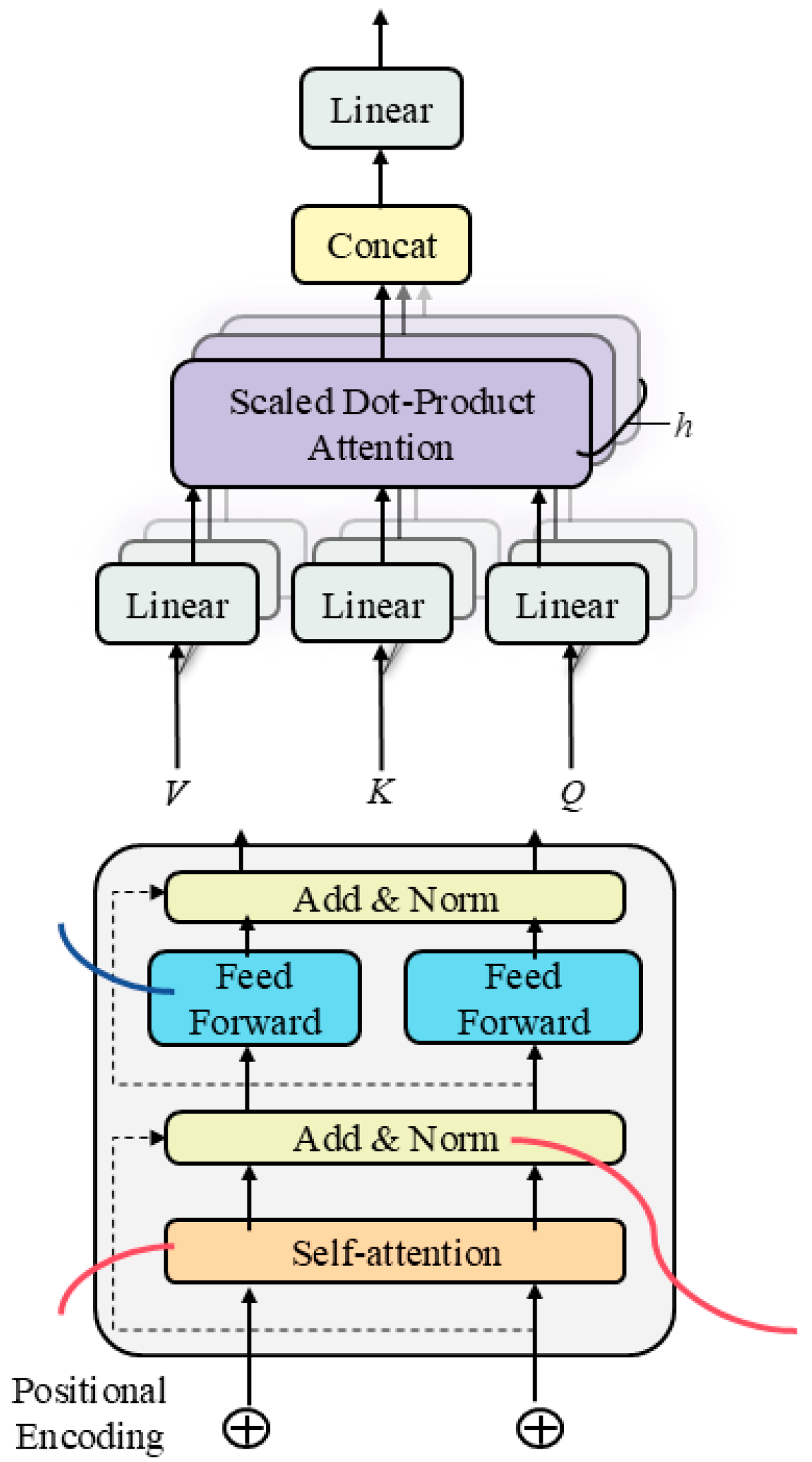
Figure 1. Schematic diagram of the Transformer–Multiple Attention mechanism.
Processes 13 03459 g001
Figure 2. Schematic diagram of GRU.
Processes 13 03459 g002
Figure 3. Schematic diagram of BiGRU.
Processes 13 03459 g003
Figure 4. Schematic diagram of global attention.
Processes 13 03459 g004
Figure 5. Schematic diagram of the cross-attention mechanism.
Processes 13 03459 g005
Figure 6. Schematic diagram of the Transformer–BiGRU–GlobalAttention model.
Processes 13 03459 g006
Figure 7. Visualization of ETT data samples.
Processes 13 03459 g007
Figure 8. Visualization of MSE loss convergence between training and testing sets.
Processes 13 03459 g008
Figure 9. Prediction performance on the dataset.
Processes 13 03459 g009
Figure 10. Feature contribution analysis.
Processes 13 03459 g010
Table 1. Description of features in the dataset.
FieldDateHUFLHULLMUFLMULLLUFLLULLOT
DescriptionRecord dateHigh useful loadHigh useless loadMedium useful loadMedium useless loadLow useful loadLow useless loadOil temperature (target)
UnitMWMWMWMWMWMWMW°C
Table 2. Sample of ETT data.
DateHUFL (MW)HULL (MW)MUFL (MW)MULL (MW)LUFL (MW)LULL (MW)OT (°C)
1 July 2016 0:0041.13012.48036.5369.3544.4231.31038.662
1 July 2016 1:0037.52710.13533.9367.5324.4341.21537.124
1 July 2016 2:0037.94611.30935.3309.0062.1000.00036.465
1 July 2016 3:0038.95111.89535.5439.4353.3801.21533.608
1 July 2016 4:0038.11311.47535.4099.6232.0360.00031.850
Table 3. Model parameter settings.
Module NameParameterValue
TransformerAttention Dimension128
Encoder Layers2
Cross-AttentionMulti-Head Attention Heads2
BiGRULayers32
Dimension64
Global Attention DimensionAttention Layer Dimension64
HyperparametersLearning Rate0.003
Loss FunctionMSE
Dropout0.5
OptimizerAdam
Table 4. Comparative results of this method with other methods.
MethodMSEMAERMSEMAPER2
LSTM [24]0.1550.30714.948.50.86
ARIMA [25]3.5540.44514.7712.10.87
CNN [26]0.1970.35712.617.80.90
Prophet [27]0.1990.38113.539.20.88
Informer [28]0.0930.24013.716.50.92
AE-BiLSTM [29]0.1070.27412.456.80.91
CNN-BiGRU-Attention [30]0.0870.25512.376.00.93
Transformer-LSTM [31]0.0830.24612.215.50.94
Transformer-BiGRU-GlobalAttention0.0780.23311.134.80.95
Table 5. Results of ablation experiments.
MethodMSEMAERMSE
Transformer0.0970.24613.12
BiGRU0.0930.24112.87
Transformer+BiGRU0.0850.23712.59
Transformer–BiGRU–GlobalAttention0.0780.23311.13
Disclaimer/Publisher’s Note: The statements, opinions and data contained in all publications are solely those of the individual author(s) and contributor(s) and not of MDPI and/or the editor(s). MDPI and/or the editor(s) disclaim responsibility for any injury to people or property resulting from any ideas, methods, instructions or products referred to in the content.