Abstract
The integrity of natural gas pipelines will decrease with an increase in operating time, thus causing pipeline leaks and accidents. However, it is challenging to improve the precision and automation of existing sensors to raise leak prediction and classification precision. Therefore, based on deep learning, a 1D convolutional neural network (CNN) incorporating the channel attention mechanism is proposed for recognizing and classifying the type of natural gas pipeline leakage. Firstly, the data reconstruction of the leaked acoustic signals, which have been classified by energy modes, is performed by feature augmentation and Bessel filtering. Subsequently, a lightweight CNN is proposed, and an attention mechanism is introduced to optimize the model performance. The results show that the training performance of the network with the attention mechanism is superior to that of the original network and the network with batch normalization. The attention mechanism network is then used to train the leakage signals with different features of engineering parameters. Finally, the test accuracy achieves 97.81%, validating the effectiveness of the proposed method for identifying and classifying natural gas leaks. It presents new ideas for the implementation of deep learning in the natural gas and chemical industries.
1. Introduction
While long and intricate natural gas pipelines provide public convenience, they also bring challenges in terms of system integrity and reliability [1]. The medium in the pipeline is usually flowing under high pressure. In the event of leakage, large amounts of hazardous gas will be released, which may cause serious secondary disasters (e.g., toxicity, fires, explosions, etc.) [2]. Therefore, timely monitoring of natural gas pipelines is an effective measure to prevent accidents. This is particularly important in view of current proposals to introduce hydrogen into natural gas pipelines [3], and fault monitoring of leaks in high-pressure pipelines should attract more attention.
Numerous studies have been conducted to develop innovative methods for the effective detection and monitoring of natural gas leakage. In conventional natural gas pipeline leakage monitoring methods, sensors are mainly used to detect changes in environmental data and determine whether the system has faults by comparing the original state. In the early period, Xia et al. [4] introduced a gas-monitoring technique based on tunable diode laser absorption spectroscopy (TDLAS), in which a diode laser was employed to detect methane and hydrogen sulfide within natural gas. Furthermore, subsequent studies have incrementally enhanced the reliability of TDLAS sensors for the monitoring of natural gas leaks. [5]. In later research, Zhang et al. [6] detailed a gas leak detection system that employs direct absorption spectroscopy with scanning wavelengths, specifically designed for the monitoring of methane and hydrogen sulfide emissions. Zhang et al. [7] proposed an omnidirectional methane sensor based on spectroscopic techniques for leak detection in explosion-hazardous environments. Moreover, a time-division scanning-assisted wavelength modulation spectroscopy (WMS) technique was used for concurrent acetylene monitoring [8]. Mukherjee et al. [9] examined a gas sensor that operates on the principle of dielectric breakdown for the identification of leakage gases and incorporated a temperature sensor to augment its monitoring capabilities. In order to improve the efficiency and accuracy of methane leakage monitoring, Meng et al. [10] devised a forward prediction model for methane concentration, which is capable of precisely tracking 30% of the methane concentration within a radius of 6 m. Yang et al. [11] employed infrared thermography to identify the position and flow rate of gas leaks by analyzing the temperature field surrounding the leakage source. Miao and Zhao [12] a multisource and heterogeneous information fusion method that integrates laser optical sensing with weak magnetic techniques to overcome the challenge of insufficient accuracy associated with current single-sensor leakage detection methods. However, traditional monitoring methods tend to be costly to implement and complicated to integrate into existing systems. Meanwhile, relying solely on a single threshold value to assess the occurrence of a leak introduces a high level of uncertainty.
In recent years, as artificial intelligence technology advances and computational capabilities are enhanced, the application of machine learning within urban construction and engineering sectors has expanded incrementally. Based on machine learning methods, novel concepts have emerged for natural gas leak monitoring [13]. Vanitha et al. [14] demonstrated that machine learning technology can accurately classify risks without delay. Aromoye et al. [15] conducted a comprehensive review of UAV–based pipeline inspection technologies, with particular emphasis on enhancing leak-detection accuracy through advanced artificial intelligence approaches. Tian et al. [16] demonstrated that the detection accuracy of their final model exceeded 90% following the integration of an extreme learning machine for training purposes, utilizing pressure signals from leaks. This approach offers superior accuracy and efficiency relative to Support Vector Machines (SVM) and Back Propagation Neural Network (BPNN). Ma et al. [17] reviewed computer vision (CV)-based defect inspection technologies and emphasized how advanced learning models, including Transformer and semi-supervised learning methods, can improve the accuracy of visual leak and defect detection, thereby promoting more intelligent and proactive pipeline maintenance. Cruz et al. [18] demonstrated that the random forest model achieved the highest performance in identifying leakages, with an error rate as low as 0.3%.
However, machine learning methods will face challenges when dealing with complex nonlinear problems. As a branch of machine learning, the multi-layer neural networks of deep learning are able to capture more complex patterns and connections in the data.
Based on deep learning theory, Beak et al. [19] constructed a deep learning network for the prediction of gas leakage by decomposing the complex regression problem into sub-problems of classification and regression to boost the efficiency of the model. Tao et al. [20] combined neural networks to evaluate leakage risk, integrating both internal and external features to facilitate the timely identification of potential leakage locations. Zhu et al. [21] discovered that the nonlinear and irregular characteristics of leakage signals inside valves can be well examined through the Deep Belief Network (DBN) models. CNN and Recurrent Neural Network (RNN) favor addressing complex, nonlinear time series challenges within the domain of deep learning. As Zuo et al. [22] optimized a long short-term memory network by an autoencoder to reduce the dependence of leakage detection methods on leakage data. The leakage features are learned through the Long-Short Term Memory and AutoEncoder (LSTM-AE) network, and then the score of the leakage is calculated by SVM. The results verify that the algorithm attains high precision in the actual dataset. However, RNNs are prone to issues including gradient vanishing and gradient exploding during training, as well as exhibiting slow convergence [23]. To overcome these issues, LSTM was introduced [24]. For instance, Zhang et al. [25] proposed an LSTM method based on an attention mechanism for the localization of individual leaks in a branch network, which can accurately capture the physical pressure changes detected by the sensor. For time series problems, a 1D CNN can achieve the same effect as an RNN. Xu et al. [26] classified ambient sounds via a 1D CNN network, which exhibited good performance in resource-constrained applications by a lightweight network model. Moreover, Yao et al. [27] demonstrated excellent performance by using a one-dimensional convolutional neural network to classify natural gas leakage data with an accuracy of 95.17%.
There are other explorations of employing deep learning for gas leakage monitoring. In this paper, we rely on existing datasets and augment them with features. Initially, we relied on existing datasets and classified the entire dataset using energy clustering methods from previous studies. In the feature engineering approach, we applied feature augmentation and Bessel filtering on low-energy and high-energy data, respectively, to make the data convergent. Subsequently, a deep but lightweight convolutional network combined with an attention mechanism is proposed, and the prediction performance of the model for leakage signals is analyzed and discussed for each parameter. Finally, the performance of the hybrid CNN–LSTM network is discussed. The results extend the applicability and robustness of deep learning techniques for natural gas leakage monitoring.
Although this paper improved the prediction accuracy to 97.81% on this dataset, the performance on low-energy data still needs enhancement. Further validation is required to determine whether reducing model parameters can achieve the same effect, as well as its application in real scenarios.
2. Sources of Datasets
The dataset of leakage acoustic signals was GPLA-12, which is a new dataset of leakage acoustic signals [27]. The dataset is based on the collection of a complete natural gas pipeline system and contains 684 sets in 12 categories [28].
3. Methodology
3.1. Clustering Methods for Leakage Acoustic Signals
The energy modal clustering method was proposed by Yao et al. [27], which addresses the limitations inherent in small-sample datasets, including the absence of features and high noise levels.
This approach enables the effective categorization of feature-missing data and excessive noise data, and the energy modal clustering is shown in Equation (1) [27].
where is the set of energy clusters, and represent the high-energy modal category and the low-energy modal categories.
According to the energy modal clustering analysis, Time series data is divided into two categories, low-energy modal and high-energy modal, where signal features are lacking in low-energy modal series and noise in the signal is more prominent in high-energy modal series. To address the problems, feature augmentation and noise filtering need to be performed on the signals.
3.1.1. Feature Augmentation
First, the peak augmentation is applied to the parts of the serial data where local features are missing. The feature location satisfies the determined criteria in Equation (2).
where is the series feature value, is the position corresponding to the series feature value, and when , is the location for augmentation.
The expression of the series data after local feature augmentation as shown in Equation (3).
where is the augmentation factor, , is an integer, and .
The augmentation factor ∈ [1, 1.3] is used to control the intensity of the enhancement. When = 1, the features remain unchanged; as increases, the intensity of the features also increases. The standard deviation validation confirms w ≤ 3, with the relative standard deviation < 0.30. Feature augmentation maintains the statistical properties of the data. At the same time, the absolute value remains within the scope of low-energy modal classification.
The effect of some of the time-series features after augmentation is shown in Figure 1. The local features of the acoustic signal change dynamically, and the key information in the signal is amplified, which enhances the recognition and classification performance.
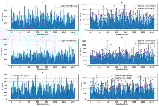
Figure 1.
Result of feature augmentation. (a) Original time series 1 (b) Feature augmentation time series 1 (c) Original time series 2 (d) Feature augmentation time series 2 (e) Original time series 3 (f) Feature augmentation time series 3.
3.1.2. Bessel Filtering
A Bessel filter is used for the distortion reduction in high-energy modal series data. The Bessel filter provides a relatively flat amplitude response in the passband compared to the Butterworth filter, which helps to minimize signal amplitude variations in the passband. Moreover, Bessel filters have a monotonically decreasing group delay, which tends to reduce phase distortion in the signal. The Bessel filter is shown in Equation (4).
where is the desired cutoff frequency, is the inverse Bessel polynomial.
Under the relatively optimal augmentation factor, Bessel filters with low-, middle-, and high-cut-off frequencies are implemented, each employing a fifth-order filter. To better preserve the temporal characteristics of the signal.
3.2. Convolutional Neural Network
Due to the excellent performance of CNN in 2D data processing, researchers have attempted to construct a 1D CNN for time series data prediction [29]. Inspired by the VGG network structure [30], this paper constructs a network structure as shown in Figure 2 and Table 1, including one input layer, six convolutional layers, three maximum pooling layers, and one global average pooling layer.
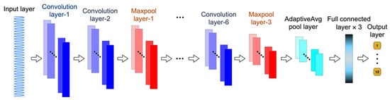
Figure 2.
Schematic diagram of 1D CNN.

Table 1.
Network details.
The structure is lightened based on the VGG structure, and the pooling operation is applied after each two convolutional operations. Finally, leakage classes are labelled by three fully connected layers and one output layer.
The data of the leakage time series is input to the CNN through the input layer with the number of input features as one.
The features in the leakage data are extracted through the convolutional layer and classified based on the data evolution patterns and trends over the whole time series. The convolutional operation process is shown in Equation (5).
where is the ith output feature in the lth layer network, is the number of output features in the previous layer, is the jth convolution kernel in layer l. is the bias.
Nonlinear properties are introduced into the neural network via the activation function, which enhances the network′s learning ability and implements the categorization. The Rectified Linear Unit (ReLU) function is employed to address the gradient vanishing [31].
The feature dimension and complexity of the CNN are decreased by pooling operations with a stride of two, while the robustness of the network is modified. Hence, the network can gradually extract higher-level abstract features that facilitate the capture of leakage features.
Average pooling is used at the end of the convolutional layer to avoid over-reliance of the network on specific features in the training data, as well as to reduce the network′s sensitivity to specific locations in the signal [32].
The ability of the network to recognize leakage faults is strengthened by the combination of local features into global features through the three fully connected layers.
The final prediction results are obtained by the output layer.
3.3. Optimized Design of the Model
3.3.1. Batch Normalization (BN)
The use of the BN layer accelerates the convergence of the network and reduces the gradient vanishing problem; in addition, it reduces the overfitting phenomenon of the network [33].
The BN layer is inserted between two equal convolutional layers.
3.3.2. Dropout Process
Figure 3 illustrates that during training, half of the neurons are randomly dropped to prevent overfitting as the network depth increases, as expressed in Equation (6).
where and is the Parameter value at time t and t0. t is the time. N is the total time steps.
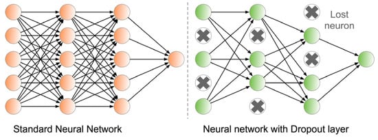
Figure 3.
Schematic diagram of dropout layer principle.
The dropout layer is inserted between fully connected layers.
3.3.3. Channel Attention (CA)
In CNN, the importance of each channel is adjusted by weight, which emphasizes the important feature channels and suppresses the unimportant ones for augmenting the feature representation [34]. Therefore, a channel attention mechanism, as shown in Figure 4, is inserted into the CNN to realize the extraction of key features of gas leakage.
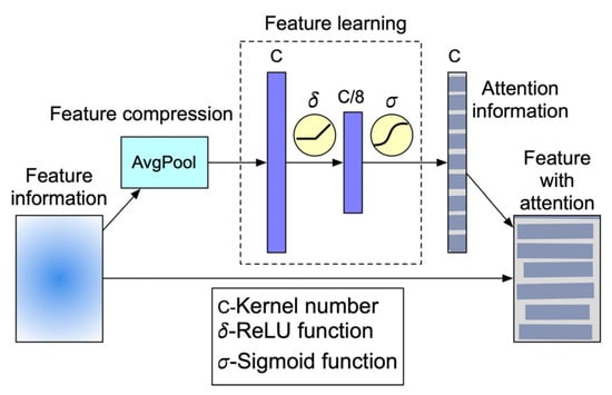
Figure 4.
Schematic diagram of the channel attention mechanism.
The features of each channel are first compressed into a single real number using global average pooling, which captures global distributional information. The dependence between channels is learned, and the weights are generated for each channel by means of a fully connected layer accompanied by an activation function. The expression is shown in Equation (7).
where and are the weights, δ is the ReLU function, σ is the Sigmoid function, and z is the global average pooling function.
where is the dimension, and is the ith element order.
The learned weights are weighed to the original features through Equation (9)
where is the channel after adjusting the weights. is the weight.
The CA layer is inserted between the convolutional layer and the pooling layer. It simultaneously replaces the role of the fully connected layer within the network.
4. Model Training
The training process of the model is shown in Figure 5. The time series data was divided into training and test sets in the ratio of 8:2. The training batch size was set to 128. The difference between the prediction and the true labels was quantified by the Cross-Entropy Loss Function. Additionally, the Adaptive Moment Estimation (Adam) was adopted with the learning rate of 0.0001. The training was set up for 100 epochs, and the optimal parameters were saved when completion. The model was implemented using Python code and built using PyTorch 2.4, and it was trained on an Intel Core i7-12700 with an NVIDIA GeForce 3060 Ti platform.
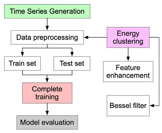
Figure 5.
Process of neural network training.
The performance of the model is assessed by the accuracy, precision, recall, and F1 scores, which are expressed by Equations (10)—(13).
where TP is true positives, FP is false positives, FN is false negatives, and TN is true negatives.
The true positive rate and false positive rate are expressed by Equations (14) and (15)
5. Model Performance and Evaluation
The aim of this study is to match the best combination of parameters to reconstruct the leakage signal dataset and to adapt the custom CNN to accurately predict the leakage signal.
Figure 6 illustrates the learning process of a customized CNN on the GPLA-12 dataset. In Figure 6a, the loss function gradually decreases, and the model predictions gradually approach the true labels. However, the loss value declines slowly as it approaches 0.6 and no longer has a significant downward trend. In comparison to the change in accuracy during the training process (see Figure 6b), the prediction accuracy shows an oscillating upward trend. As the loss values stabilize, the trend in accuracy similarly decreases and does not rise. This indicates that the customized CNN can acquire leakage features for prediction. Yet, based on the trend of the accuracy curve, it is concluded that the predictive capability still needs to be advanced. Therefore, the batch normalization and dropout layers were inserted behind the convolutional layers and retrained.
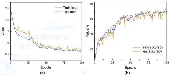
Figure 6.
Dynamic results of CNN. (a) Loss value (b) accuracy.
Figure 7 shows the results of adding the batch normalization layer to the convolutional layer and the dropout layer to the fully connected layer. The parameters are updated more efficiently compared to the initial network structure. The value of loss in Figure 7a can decrease rapidly, which suggests that the model can converge quickly and close to 0.5. As the loss value decreases, the model accuracy of prediction improves. Figure 7b reveals that the accuracy is in a range above 80%. The reason for this analysis is that the optimized model captures the more general patterns of the dataset, and the loss function escapes from local minimums. Thus, it is concluded that adding a batch normalization layer and a dropout layer can improve the network′s accuracy in predicting leakage signals.
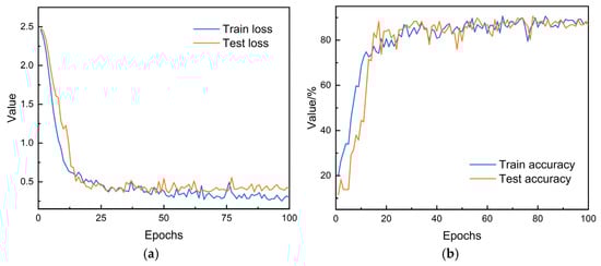
Figure 7.
Dynamic results of CNN + BN + dropout layers. (a) Loss value (b) accuracy.
The attention mechanism is adopted to replace the fully connected layer in CNN, so as to achieve the refinement of network parameters [35]. At the same time, the dependency relationship between channels is constructed through the attention mechanism to distinguish the weights. Figure 8 shows the results of the network with the channel attention mechanism. Figure 8a reveals that the loss function drops to a lower value, the model converges to a more optimal solution, and the network prediction accuracy improves slightly (see Figure 8b).
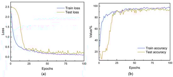
Figure 8.
Dynamic results of CNN + CA. (a) Loss value (b) accuracy.
Figure 9 shows the training results of adding BN and CA to the CNN. The distribution of BN outputs fluctuates, which leads to an unstable basis for the calculation of attention weights. Conversely, the redistribution of attention weights changes the feature distribution of subsequent BN layers, affecting the statistics estimation of BN layers. This amplifies the impact of minor features, causing unstable results.
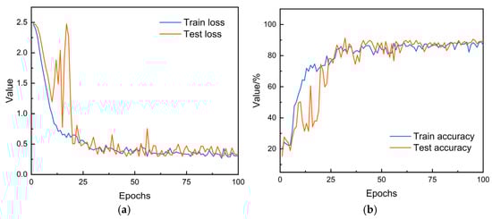
Figure 9.
Dynamic results of CNN + BN + dropout layers + CA. (a) Loss value (b) accuracy.
Table 2 lists the accuracy achieved on the test set using the optimal training parameters for different structures in a single run. The BN layer and the dropout layer will improve the prediction potential of the network, but there is still no optimal solution to be desired (There is a gap with the results of Yao et al. [27]). The reason for this analysis is that the loss function may have multiple local minimums, and this accuracy is not sufficient for the current research. The inclusion of the attention mechanism allows the network to learn the emphasis of different feature channels and adjust the feature weights. This method enables us to strengthen the representation of valuable features with less parameters. It has better performance with fewer parameters.
Table 2.
Optimal training parameters for different network structures.
Based on the training results of different network structures, the CNN with an attention mechanism is used to train and learn the reconstructed leakage signal data. The accuracy of prediction for different multiples of feature augmentation in low-energy modal data is shown in Figure 10. Notably, the accuracy achieves 97.08% as the feature augmentation value is 1.1 times. There is an improvement compared to the original dataset. The reason for this is that the peaks of the time series tend to characterize important information, and the networks will capture variations in features more robustly with an attention mechanism. But the accuracy decreases when the feature magnification is scaled up to 1.2 and 1.3 times. The reason for this is that too large a feature augmentation factor may introduce too much noise, which can lead to degradation of the model performance.
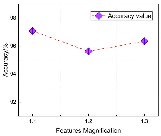
Figure 10.
Test accuracy of feature-augmented dataset.
Further filtering parameters for high-energy modal data are selected based on the feature augmentation training results. The network training accuracy at different cutoff frequencies is shown in Figure 11, the network training parameters are best, and the prediction accuracy achieves 97.81% as the cutoff frequency is 0.5. There is a significant improvement in the accuracy of gas leakage prediction compared to previous studies. It is verified that the custom CNN with the reconstructed dataset from the improved energy clustering method provides better representation ability. The model can converge to a well-performing minimum under the attention mechanism. And the cutoff frequency should not be too large or too small for noise reduction of high-energy modal.
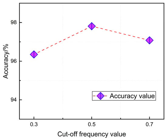
Figure 11.
Test accuracy of low-pass filtered dataset.
Comparing the training results (Figure 12) in terms of accuracy, recall, and F1 score reveals that the model maintains good predictive accuracy while fully capturing all positive examples. However, as the recall for Class 3 and Class 5 decreased, the precision correspondingly dropped to 0.86 and 0.8. The results indicate that the model performs well on high-energy mode data but loses accuracy on low-energy mode data, which prompts the conclusion that the model has limited ability to distinguish between low-energy data classes. The overall performance of the model will be quantified using the ROC curve in subsequent phases.
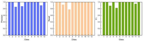
Figure 12.
Precision, recall, and F1 scores of CNN-CA.
In previous models, significant classification confusion was observed for classes 1, 3, and 6 [27]. The model proposed in this study overcomes this issue, and Figure 13 presents the inference results of the optimal parameters. The classification accuracy is significantly higher than previous models, indicating that its feature extraction and classification algorithms are more effective. In the confusion matrix, the network has a good generalization ability to high-energy modal categories, and all of them can accurately predict the true label. Although the model demonstrates stronger generalization ability and stability, in the low-energy modal class, the prediction accuracy for individual classes has decreased. This suggests that further feature engineering efforts need to be strengthened to enhance the prediction accuracy for low-energy modal or to improve the network structure in a targeted manner. This is one of our future research priorities.
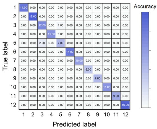
Figure 13.
Confusion matrix of accuracy with CNN-CA.
Figure 14 shows that the model has good distinction ability for 12 classes. The macro average (AUC) value of 1.00 indicates that the average performance of the model at the category level has reached the theoretical optimal level, and this evaluation is unaffected by any potential imbalance in the number of samples. Only Class 3 (AUC = 0.98) and Class 5 (AUC = 0.99) are slightly below 1.00. This indicates that the model demonstrates only extremely minimal errors for these two classes, maintaining reliable performance.
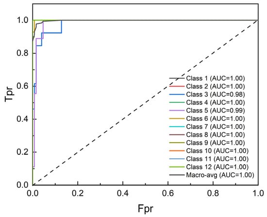
Figure 14.
ROC of CNN–CA.
6. Discussions
Since CNN and LSTM emphasize different feature representations. Finally, we discuss the embedding of an LSTM within a 1D CNN to achieve joint learning, i.e., learning long-term dependencies between time steps via the LSTM. The LSTM layer, with layer number 1, is supplemented after the convolutional layer. Through a detailed analysis of each metric in Figure 15, it is identified that the hybrid model exhibits performance shortcomings in specific classes (such as classes 3, 4, 5, and 8), specifically manifested as insufficient precision and recall rates. The result of the overall inference is shown in Figure 16. It can be concluded that the accuracy performs the same as the CNN-Attention in accuracy (97.81%). The difference is that there is a variation in the accuracy of identification of leakage classes, but the trend remains that there will be a decline in the accuracy of low-energy modal classes. Therefore, the performance that the hybrid network provides can already be achieved by the data reconstruction and lightweight CNN proposed in this paper, and a redundant stacking of the network structure is no longer required.
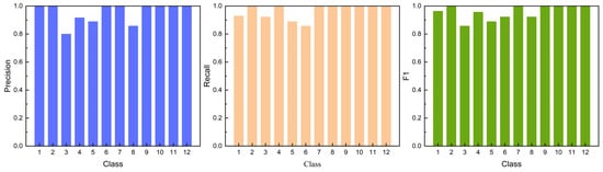
Figure 15.
Precision, recall, and F1 scores of CNN–LSTM–CA.

Figure 16.
Confusion matrix of accuracy with CNN–LSTM–CA.
Based on the quantitative metrics provided (Figure 17), there is no significant difference in performance between the two models. They all achieved similar classification capabilities. Whether in overall macro-level performance or in the ability to identify various classes at the micro level, lightweight models demonstrate equally good performance.
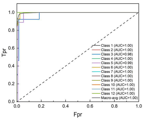
Figure 17.
ROC of CNN–LSTM–CA.
7. Limitations
Although experimental settings enable precise variable control, the ability to capture the complexity and unpredictability of real environments is yet to be verified. Furthermore, only a limited amount of noise and pipe scale is introduced during training, and the generalizability of these findings to other conditions requires further investigation. Based on the limitations, we have defined the next steps: conducting field validation to assess its performance under realistic conditions and optimizing the model.
8. Conclusions and Outlook
This paper proposes a lightweight convolutional neural network that incorporates a channel attention mechanism during the classification stage to highlight important feature channels. Feature engineering for energy clustering methods has been enhanced. Feature peaks in low-energy modes have been amplified, while high-energy modes have been applied with Bessel low-pass filtering to stabilize feature distribution.
The proposed CNN achieves rapid convergence and high accuracy (97.81%) in natural gas leakage prediction and classification, with overall performance (AUC) approaching that of hybrid networks while maintaining low computational complexity. This model not only has competitive accuracy but also demonstrates advantages in efficiency and deployment.
Future work will extend the range of feature engineering values and incorporate frequency-domain features to enhance the model’s adaptability and generalization capabilities under complex operating conditions, ultimately contributing to the development of intelligent and proactive pipeline safety management systems.
Author Contributions
Writing—review and editing, Z.C.; Data curation, Z.G.; Investigation, L.Q. Project administration, H.M.; Funding acquisition, H.M.; Methodology, C.Z.; Formal analysis, H.Z.; Visualization, X.F.; Resources, T.S.; Supervision, K.W.; Validation, X.W.; Writing—original draft, S.W. All authors have read and agreed to the published version of the manuscript.
Funding
This research was funded by National Natural Science Foundation of China (52274177) and the Chongqing Construction Science and Technology Programme (2024–0146).
Data Availability Statement
The original data presented in the study are openly available at https://arxiv.org/abs/2106.10277 (accessed on 1 September 2025).
Conflicts of Interest
Authors Zhi Chen, Zhibing Gu, Long Qin were employed by the company Sichuan Changning Natural Gas Development Co., Ltd. Authors Changlin Zhou, Xingzheng Feng, Tao Song, Ke Wu were employed by the company Sichuan Shengnuo Oil and Gas Engineering Technology Service Co., Ltd. Author Xin Wang was employed by the company Southwest Oil and Gas Field Branch of China National Petroleum Corporation. The remaining authors declare that the research was conducted in the absence of any commercial or financial relationships that could be construed as a potential conflict of interest.
References
- Feng, Y.; Gao, J.; Yin, X.; Chen, J.; Wu, X. Risk assessment and simulation of gas pipeline leakage based on Markov chain theory. J. Loss Prev. Process Ind. 2024, 91, 105370. [Google Scholar] [CrossRef]
- Zeng, F.; Jiang, Z.; Zheng, D.; Si, M.; Wang, Y. Study on numerical simulation of leakage and diffusion law of parallel buried gas pipelines in tunnels. Process Saf. Environ. Prot. 2023, 177, 258–277. [Google Scholar] [CrossRef]
- Han, H.; Chang, X.; Duan, P.; Li, Y.; Zhu, J.; Kong, Y. Study on the leakage and diffusion behavior of hydrogen-blended natural gas in utility tunnels. J. Loss Prev. Process Ind. 2023, 85, 105151. [Google Scholar] [CrossRef]
- Xia, H.; Liu, W.; Zhang, Y.; Kan, R.; Wang, M.; He, Y.; Cui, Y.; Ruan, J.; Geng, H. An approach of open-path gas sensor based on tunable diode laser absorption spectroscopy. Chin. Opt. Lett. 2008, 6, 437–440. [Google Scholar] [CrossRef]
- You, K.; Zhang, Y.J.; Wang, L.M.; Li, H.; Li, H.B.; He, Y. Improving the Stability of Tunable Diode Laser Sensor for Natural Gas Leakage Monitoring. Adv. Mat. Res. 2013, 760–762, 84–87. [Google Scholar] [CrossRef]
- Zhang, S.; Liu, W.; Zhang, Y.; Shu, X.; Yu, D.; Kan, R.; Dong, J.; Geng, H.; Liu, J. Gas leakage monitoring with scanned-wavelength direct absorption spectroscopy. Chin. Opt. Lett. 2010, 8, 443–446. Available online: https://opg.optica.org/col/abstract.cfm?uri=col-8-5-443 (accessed on 1 September 2025). [CrossRef]
- Zhang, L.; Pang, T.; Zhang, Z.; Sun, P.; Xia, H.; Wu, B.; Guo, Q.; Sigrist, M.W.; Shu, C. A novel compact intrinsic safety full range Methane microprobe sensor using “trans-world” processing method based on near-infrared spectroscopy. Sens. Actuators B Chem. 2021, 334, 129680. [Google Scholar] [CrossRef]
- Zhang, L.; Zhang, Z.; Sun, P.; Pang, T.; Xia, H.; Cui, X.; Guo, Q.; Sigrist, M.W.; Shu, C.; Shu, Z. A dual-gas sensor for simultaneous detection of methane and acetylene based on time-sharing scanning assisted wavelength modulation spectroscopy. Spectrochim. Acta A Mol. Biomol. Spectrosc. 2020, 239, 118495. [Google Scholar] [CrossRef] [PubMed]
- Mukherjee, T.; Paul, A. Dielectric Breakdown-Based Gas Leakage Detector Using Poly-Si Microtips. IEEE Trans. Electron. Devices 2018, 65, 5029–5037. [Google Scholar] [CrossRef]
- Meng, G.; Hu, H.; Qiu, Y.; Chen, S.; Gu, S.; Chang, X.; Du, S. Natural gas leakage: Forward and inverse method of leakage field based on multipath concentration monitoring. Measurement 2025, 240, 115494. [Google Scholar] [CrossRef]
- Yang, H.; Yao, X.F.; Wang, S.; Yuan, L.; Ke, Y.C.; Liu, Y.H. Simultaneous determination of gas leakage location and leakage rate based on local temperature gradient. Measurement 2019, 133, 233–240. [Google Scholar] [CrossRef]
- Miao, X.; Zhao, H. Leakage diagnosis of natural gas pipeline based on multi-source heterogeneous information fusion. Int. J. Press. Vessel. Pip. 2024, 209, 105202. [Google Scholar] [CrossRef]
- Lu, H.; Iseley, T.; Behbahani, S.; Fu, L. Leakage detection techniques for oil and gas pipelines: State-of-the-art. Tunn. Undergr. Space Technol. 2020, 98, 103249. [Google Scholar] [CrossRef]
- Vanitha, C.N.; Easwaramoorthy, S.V.; Krishna, S.A.; Cho, J. Efficient qualitative risk assessment of pipelines using relative risk score based on machine learning. Sci. Rep. 2023, 13, 14918. [Google Scholar] [CrossRef]
- Aromoye, I.A.; Lo, H.H.; Sebastian, P.; Abro, G.E.M.; Ayinla, S.L. Significant Advancements in UAV Technology for Reliable Oil and Gas Pipeline Monitoring. CMES Comput. Model. Eng. Sci. 2025, 142, 1155–1197. [Google Scholar] [CrossRef]
- Tian, X.; Jiao, W.; Liu, T.; Ren, L.; Song, B. Leakage detection of low-pressure gas distribution pipeline system based on linear fitting and extreme learning machine. Int. J. Press. Vessel. Pip. 2021, 194, 104553. [Google Scholar] [CrossRef]
- Ma, D.; Fang, H.; Wang, N.; Hu, H.; Jiang, X. The state-of-the-art in pipe defect inspection with computer vision-based methods. Measurement 2026, 257, 118431. [Google Scholar] [CrossRef]
- da Cruz, R.P.; da Silva, F.V.; Fileti, A.M.F. Machine learning and acoustic method applied to leak detection and location in low-pressure gas pipelines. Clean Technol. Environ. Policy 2020, 22, 627–638. [Google Scholar] [CrossRef]
- Baek, S.; Bacon, D.H.; Huerta, N.J. Enabling site-specific well leakage risk estimation during geologic carbon sequestration using a modular deep-learning-based wellbore leakage model. Int. J. Greenh. Gas Control 2023, 126, 103903. [Google Scholar] [CrossRef]
- Tao, T.; Deng, Z.; Chen, Z.; Chen, L.; Chen, L.; Huang, S. Intelligent Urban Sensing for Gas Leakage Risk Assessment. IEEE Access 2023, 11, 37900–37910. [Google Scholar] [CrossRef]
- Zhu, S.B.; Li, Z.L.; Zhang, S.M.; Ying, Y.; Zhang, H.F. Deep belief network-based internal valve leakage rate prediction approach. Measurement 2019, 133, 182–192. [Google Scholar] [CrossRef]
- Zuo, Z.; Ma, L.; Liang, S.; Liang, J.; Zhang, H.; Liu, T. A semi-supervised leakage detection method driven by multivariate time series for natural gas gathering pipeline. Process Saf. Environ. Prot. 2022, 164, 468–478. [Google Scholar] [CrossRef]
- Rehmer, A.; Kroll, A. On the vanishing and exploding gradient problem in Gated Recurrent Units. IFAC-PapersOnLine 2020, 53, 1243–1248. [Google Scholar] [CrossRef]
- Hochreiter, S.; Schmidhuber, J. Long Short-Term Memory. Neural Comput. 1997, 9, 1735–1780. [Google Scholar] [CrossRef]
- Zhang, X.; Shi, J.; Yang, M.; Huang, X.; Usmani, A.S.; Chen, G.; Fu, J.; Huang, J.; Li, J. Real-time pipeline leak detection and localization using an attention-based LSTM approach. Process Saf. Environ. Prot. 2023, 174, 460–472. [Google Scholar] [CrossRef]
- Xu, H.; Tian, Y.; Ren, H.; Liu, X. A Lightweight Channel and Time Attention Enhanced 1D CNN Model for Environmental Sound Classification. Expert Syst. Appl. 2024, 249, 123768. [Google Scholar] [CrossRef]
- Yao, L.; Zhang, Y.; He, T.; Luo, H. Natural gas pipeline leak detection based on acoustic signal analysis and feature reconstruction. Appl. Energy 2023, 352, 121975. [Google Scholar] [CrossRef]
- Liao, H.; Zhu, W.; Zhang, B.; Zhang, X.; Sun, Y.; Wang, C.; Li, J. Application of Natural Gas Pipeline Leakage Detection Based on Improved DRSN-CW. In Proceedings of the 2021 IEEE International Conference on Emergency Science and Information Technology, Chongqing, China, 22–24 November 2021; pp. 514–518. [Google Scholar] [CrossRef]
- Kim, Y. Convolutional Neural Networks for Sentence Classification. In Proceedings of the 2014 Conference on Empirical Methods in Natural Language Processing (EMNLP), Doha, Qatar, 25–29 October 2014; pp. 1746–1751. [Google Scholar] [CrossRef]
- Simonyan, K.; Zisserman, A. Very Deep Convolutional Networks for Large-Scale Image Recognition. In Proceedings of the 3rd International Conference on Learning Representations. arXiv 2014, arXiv:1409.1556v6. Available online: https://api.semanticscholar.org/CorpusID:14124313 (accessed on 1 September 2025).
- Petersen, P.; Voigtlaender, F. Optimal approximation of piecewise smooth functions using deep ReLU neural networks. Neural Netw. 2018, 108, 296–330. [Google Scholar] [CrossRef]
- Lin, M.; Chen, Q.; Yan, S. Network in Network. In Proceedings of the 2nd International Conference on Learning Representations. arXiv 2013, arXiv:1312.4400v3. Available online: http://arxiv.org/abs/1312.4400 (accessed on 1 September 2025).
- Ioffe, S.; Szegedy, C. Batch Normalization: Accelerating Deep Network Training by Reducing Internal Covariate Shift. In Proceedings of the 32nd International Conference on Machine Learning. arXiv 2015, arXiv:1502.03167v3. Available online: https://arxiv.org/abs/1502.03167 (accessed on 1 September 2025).
- Xu, Z.; Jia, Z.; Wei, Y.W.; Zhang, S.; Jin, Z.; Dong, W. A strong anti-noise and easily deployable bearing fault diagnosis model based on time–frequency dual-channel Transformer. Measurement 2024, 236, 115054. [Google Scholar] [CrossRef]
- Brauwers, G.; Frasincar, F. A General Survey on Attention Mechanisms in Deep Learning. IEEE Trans. Knowl. Data Eng. 2023, 35, 3279–3298. [Google Scholar] [CrossRef]


Disclaimer/Publisher’s Note: The statements, opinions and data contained in all publications are solely those of the individual author(s) and contributor(s) and not of MDPI and/or the editor(s). MDPI and/or the editor(s) disclaim responsibility for any injury to people or property resulting from any ideas, methods, instructions or products referred to in the content. |
© 2025 by the authors. Licensee MDPI, Basel, Switzerland. This article is an open access article distributed under the terms and conditions of the Creative Commons Attribution (CC BY) license (https://creativecommons.org/licenses/by/4.0/).