Optimization of Fine Milling Process Parameters for Small Impeller

Abstract

Addressing the issues of surface machining quality and residual stress in small impellers, the outward opening integral small impeller was selected as the key research object, and the main evaluation indicators of the surface quality of the experiment were set as the surface roughness and residual stress. The finite element simulation technology was used to analyze how the process parameters can affect the residual stress and outer surface roughness of the small impeller. After obtaining the results, the genetic algorithm was used to optimize it to obtain the optimal combination of process parameters. The surface roughness is reduced by 34.2%, and the residual stress is reduced by 28.6%, and at the same time, proved the feasibility of the optimization of the process parameters. The numerical control machining test of the small impeller was carried out to verify the feasibility and accuracy of the process parameter optimization.

1. Introduction

Small impellers are an important component widely used in aviation, aerospace, metallurgy, petrochemicals, and other fields. Their surface quality is a key factor affecting their performance.

Rotary parts are widely used in the machinery and equipment industry and play a very important role in many fields such as aviation, aerospace, metallurgy, and petrochemicals [1]. Surface quality is a major factor affecting the working performance of small impellers, so research on surface quality issues has attracted widespread attention both domestically and internationally. Compared with other countries with mature processing technologies, there are still many problems in the production and manufacturing of small impellers in China. Achieving high-quality processing of small impellers is currently the top priority in solving processing problems.

Small impellers, characterized by thin blades, large, curved surface twist angles, and deep, narrow flow channels, are classified as typical complex curved surface components that are difficult to machine [2]. During the production and machining of small impellers, the selection of process parameters directly affects the surface quality and service life of the impeller. Therefore, selecting reasonable process parameters is of utmost importance throughout the entire machining process of small impellers. However, workers tend to be cautious when selecting processing parameters, primarily adjusting them based on their own processing experience rather than through scientific and effective selection. Therefore, selecting reasonable and scientific process parameters is of great significance for achieving high-quality processing and production of small impellers.

Therefore, an orthogonal experiment with process parameters as the primary influencing factors was designed in this paper. By studying the two evaluation indicators of surface quality (i.e., surface roughness and residual stress), the paper investigated the variation regularity of these indicators under the influence of process parameters; using surface roughness and residual stress as optimization objectives, a multi-objective optimization mathematical model was constructed. This model was optimized using a genetic algorithm to obtain the optimal combination of process parameters. This set of process parameters is applied to the CNC machining of small impellers to improve the surface machining quality of small impellers and provide guidance for their production and machining.

2. Materials and Methods of Research

2.1. The Material Composition and Structural Configuration of the Small Impeller

The small impeller investigated in this study consists of nine sets of main blades and nine sets of splitter blades. Its structural dimensions are as follows: the upper diameter is 5.4 mm, the lower diameter is 32 mm, and the impeller height is 9.9 mm. The trailing edge height of the blades is 1.9 mm, with a thickness of 0.2 mm, while the distance between the main and splitter blades is 1.7 mm. The filet radius is 0.5 mm, and the impeller is made of 7075 aluminum alloy. The fundamental structural dimensions and the three-dimensional solid model of the small impeller are shown in Figure 1.

2.2. The Influence of Process Parameters on Milling Force and the Establishment of a Prediction Model

Due to the complex geometry of the small impeller, the machining challenges are primarily concentrated in three aspects:

(1)

Tool interference issues. The narrow space between the main and splitter blades of the small impeller often leads to significant tool–blade interference during machining, thereby affecting normal production and processing.

(2)

Machining deformation issues. The large twist angles of the blades make the impeller prone to deformation during machining. The narrow spacing between the main and splitter blades, combined with the high requirements for surface quality, increases the likelihood of tool–blade interference, which can result in machining deformation. In addition, the deep and narrow flow channels of the impeller reduce tool rigidity and may even lead to tool breakage.

(3)

Surface quality issues. Owing to the small diameter of the impeller and the narrow spacing between adjacent main and splitter blades, the tool is highly susceptible to vibration, which adversely affects the surface quality.

The processing of the small impeller is mainly divided into several key parts: rough machining of the flow channel, precision machining of the main and auxiliary blades, precision machining of the flow channel, and precision machining of the root radius [3]. Among them, the precision machining trajectory of the small impeller blades is shown in Figure 1b.

Therefore, to address the problem of unreasonable selection of process parameters during the milling of small impellers, an orthogonal experiment was designed with ap, ae, n, and fz as the four primary influencing factors. Based on finite element simulation techniques and multi-objective optimization methods, the effects of these four process parameters on surface roughness (Ra) and residual stress (σ) during the finishing process of small impellers were analyzed. Finally, a genetic algorithm was employed to optimize the process parameters, and the optimized parameters were subsequently validated through CNC machining experiments.

Given the overall structural complexity of the small impeller, numerous factors may affect the machining process. Since finite element simulation cannot account for all influencing factors, and in order to reduce computational time without compromising the accuracy of the results, the following assumptions were made in the simulation:

(1)

The workpiece material was selected from the material library as aluminum alloy, with the constitutive model defined as plastic.

(2)

Considering that tool wear is likely to occur during the simulation, the tool type was set as an elastoplastic body, with WC-type cemented carbide selected as the tool material.

(3)

The temperature was assumed constant at 20 °C, and the friction system was defined with a constant coefficient of friction of 0.6.

(4)

The workpiece material number Al7075-T6 was selected from the library, owing to its favorable plastic mechanical properties after solution treatment. The specific parameter settings used in this simulation analysis are listed in

Table 1. Machining parameters.

$\mathit{n}/\mathit{r}\cdot {\mathbf{min}}^{-1}$	${\mathit{f}}_{\mathbf{z}}/\mathbf{mm}\cdot {\mathit{z}}^{-1}$	${\mathit{a}}_{\mathit{p}}/\mathbf{mm}$	${\mathit{a}}_{\mathbf{e}}/\mathbf{mm}$	Coefficient of Friction	Temperature
8 × 103	0.16	1.25	0.15	0.1	20 °C
1 × 104	0.20	1.50	0.20
1.2 × 103	0.24	1.75	0.25
1.4 × 103	0.30	2.00	0.30

.

In the simulation process, tetrahedral elements were adopted for mesh generation. The number of mesh elements for the workpiece was set to 80,000, while that for the tool was 5000. The minimum element size of the workpiece mesh was 0.15584 mm. The detailed mesh division of the workpiece and tool is shown in Figure 1c. In addition, to ensure the accuracy and reliability of the simulation results, constraints were applied to the bottom profile of the small impeller. Specifically, the translational velocities in the X, Y, and Z directions were set to zero, i.e., all degrees of freedom were constrained. In this way, the bottom of the impeller was fixed, ensuring that the tool moved along the prescribed path while the workpiece remained stationary.

3. Results and Discussion

3.1. Orthogonal Experimental Design

To reduce the cutting force during the finishing process, obtain the optimal combination of process parameters, and ensure that the surface quality of the small impeller was at its best, the orthogonal experimental method was selected for process parameter optimization. This is because orthogonal experiments not only reduce the number of experiments but also ensure that the values of each group of factors are both global and representative.

The primary process parameters affecting the surface quality of small impellers during finishing are spindle speed $n$, feed per tooth $f_z$, axial cutting depth $a_p$, and radial cutting depth $a_e$. These four primary process parameters were selected as the influencing factors for the orthogonal experiment design, and a four-factor, four-level orthogonal experiment table was designed, as shown in

Table 2.  $L16\left(4^4\right)$ orthogonal table.

Experimental Number	$\mathit{n}/\mathit{r}\cdot {\mathbf{min}}^{-1}$	${\mathit{f}}_{\mathit{z}}/\mathbf{m}\mathbf{m}\cdot {\mathit{z}}^{-1}$	${\mathit{a}}_{\mathit{p}}/\mathbf{m}\mathbf{m}$	${\mathit{a}}_{\mathit{e}}/\mathbf{m}\mathbf{m}$
1	8 × 103	0.16	1.25	0.15
2	8 × 103	0.20	1.50	0.20
3	8 × 103	0.24	1.75	0.25
4	8 × 103	0.28	2.00	0.30
5	1 × 104	0.16	1.50	0.25
6	1 × 104	0.20	1.25	0.30
7	1 × 104	0.24	2.00	0.15
8	1 × 104	0.28	1.75	0.20
9	1.2 × 104	0.16	1.75	0.30
10	1.2 × 104	0.20	2.00	0.25
11	1.2 × 104	0.24	1.25	0.20
12	1.2 × 104	0.28	1.50	0.15
13	1.4 × 104	0.16	2.00	0.20
14	1.4 × 104	0.20	1.75	0.15
15	1.4 × 104	0.24	1.50	0.30
16	1.4 × 104	0.28	1.25	0.25

.

3.2. Simulation Experiment Design and Result Analysis

Finite element simulation technology has a high degree of automation, so finite element simulation software is used to perform simulation analysis on small impellers. However, due to the complex overall structure of small impellers, they are affected by many factors during the manufacturing process, and finite element simulation cannot take all factors into account. To reduce computer simulation time without affecting the accuracy of the results [4].

The following settings were made for the simulation:

(1)

The workpiece material was selected from the aluminum alloy library, with a plastic material constitutive model.

(2)

During the simulation process, the tool is prone to wear, so an elastoplastic material was selected as the tool type, with WC-type cemented carbide as the tool material.

(3)

The temperature remains constant at 20 °C.

(4)

The friction system is a constant value with a friction coefficient of 0.6.

(5)

The workpiece material number selected from the library is Al7075-T6, as it exhibits good plastic mechanical properties after solution treatment [5].

Finite element simulation analysis was performed on 16 different process parameter combinations in an orthogonal experiment. One blade was selected as the simulation object. The simulation was terminated when the force on the tool path stabilized after initial fluctuations. The changes in milling force in the X, Y, and Z directions were obtained. The milling force values in the three directions under different process parameter combinations are shown in

Table 3. Statistical table of milling force results.

Serial Number	$\mathit{n}$	${\mathit{f}}_{\mathit{z}}$	${\mathit{a}}_{\mathit{p}}$	${\mathit{a}}_{\mathit{e}}$	${\overline{{\mathit{F}}_{\mathit{x}}}}^{\mathit{\prime }}$	${\overline{{\mathit{F}}_{\mathit{y}}}}^{\mathit{\prime }}$	${\overline{{\mathit{F}}_{\mathit{z}}}}^{\mathit{\prime }}$	$\overline{\mathit{F}}$
1	8 × 103	0.16	1.25	0.15	3.12	27.28	15.73	31.64
2	8 × 103	0.20	1.50	0.20	5.13	32.97	11.93	35.44
3	8 × 103	0.24	1.75	0.25	3.54	33.46	13.37	36.21
4	8 × 103	0.28	2.00	0.30	4.12	37.54	18.14	41.90
5	1 × 104	0.16	1.50	0.25	4.35	27.95	11.37	11.23
6	1 × 104	0.20	1.25	0.30	3.37	30.91	9.83	32.61
7	1 × 104	0.24	2.00	0.15	5.94	33.01	13.52	36.16
8	1 × 104	0.28	1.75	0.20	7.12	27.54	19.56	34.52
9	1.2 × 104	0.16	1.75	0.30	5.96	38.61	18.45	43.20
10	1.2 × 104	0.20	2.00	0.25	4.18	35.96	13.12	38.51
11	1.2 × 104	0.24	1.25	0.20	4.96	27.32	10.97	29.86
12	1.2 × 104	0.28	1.50	0.15	7.32	23.24	9.43	26.13
13	1.4 × 104	0.16	2.00	0.20	3.15	34.54	11.23	36.46
14	1.4 × 104	0.20	1.75	0.15	4.34	37.19	13.46	39.79
15	1.4 × 104	0.24	1.50	0.30	7.46	28.12	15.93	33.17
16	1.4 × 104	0.28	1.25	0.25	3.92	35.54	9.36	36.96

.

Select the multi-factor analysis of variance function method to analyze the simulation data results in Table 3, and derive the degree of influence of the four process parameters on the milling force, as shown in Figure 2 below. Figure 2a shows the degree of influence in the X-direction, Figure 2b shows the degree of influence in the Y-direction, Figure 2c shows the degree of influence in the Z-direction and Figure 2d shows the degree of influence of milling joint force.

Based on the above analysis, we can conclude that:

-

The influence of X-direction process parameters on milling force is as follows: a_p and f_Z are the most significant, followed by n and a_e.

-

The influence of Y-direction process parameters on milling force is as follows: a_p and f_Z are the most significant, followed by a_e and n.

-

The influence of Z-direction process parameters on milling force is as follows: a_p and a_e are the most significant, followed by f_Z and n.

-

The degree of influence of process parameters on the milling force is as follows: a_p and a_e are greater, f_Z and n are next.

3.3. Establishment and Validation of a Milling Force Prediction Model

To effectively control and predict the surface quality of small impellers during the machining process, we decided to use the non-linear regression function provided by MATLAB 2020 software to construct a mathematical model of milling force. The standard formula for calculating milling force is defined as shown in Equation (1) according to the Metal Cutting Handbook [6]:

$$F_z={\displaystyle \frac{9.81C_F{f_z}^{X_{FZ}}\cdot {a_p}^{Y_{FZ}}\cdot {a_e}^{{\mu }_{FZ}}\cdot Z}{d^{q_F}\cdot n^{W_F}\cdot 60^{W_F}}}\cdot K_{FZ}(N)$$

(1)

In Equation (1): C_F is the milling force coefficient, K_FZ is the operating condition coefficient, and X_FZ, Y_FZ, Y_FZ, W_F are the indices of various cutting parameters. According to the above formula, the milling force is directly related to the four selected process parameters, and thus, it is necessary to determine the exponent corresponding to each parameter. In this experiment, considering the machining material of the small impeller and the selected cemented carbide ball-end mill, the above formula was simplified, and the resulting expression is presented in Equation (2).

$$F_z=C_F\cdot n^{W_F}\cdot {f_z}^{X_F}\cdot {a_p}^{Y_F}\cdot {a_e}^{{\mu }_F}$$

(2)

In this experiment, the processing material of the impeller and the selected carbide ball-end milling cutter were simplified and took logarithm in Equation (2), the result is shown in Equation (3):

$$\mathrm{l}\mathrm{g}{F}_Z=\mathrm{l}\mathrm{g}{C}_F+W_F\mathrm{l}\mathrm{g}n+X_F\mathrm{l}\mathrm{g}{f}_z+Y_{F}l\mathrm{g}{a}_p+{\mu }_F\mathrm{l}\mathrm{g}{a}_e$$

(3)

If $\mathit{lg}{F}_Z=F,\mathit{lg}{C}_F=u_1,W_F=u_2,X_F=u_3,Y_F=u_4,{\mu }_F=u_5,\mathit{lg}n=x_1,\mathit{lg}{f}_z=x_2,\mathit{lg}{a}_p=x_3,\mathit{lg}{a}_e=x_4$

Equation (2) can be transformed into Equation (4):

$$F=u_1+u_2{x}_1+u_3{x}_2+u_4{x}_3+u_5{x}_4$$

(4)

After substituting the 16 sets of experimental data from the orthogonal array into Equation (2), calculations were performed using a non-linear regression function. On this basis, the accurate values of each coefficient of the milling force were calculated, respectively, and prediction models for the milling forces in the X, Y, and Z directions as well as the resultant milling force were established.

The correlation coefficient of the predicted milling force in the resulting model is

μ₁ = 34.1849  μ₂ = 0.0001  μ₃ = 2.2121  μ₄ = 3.7559  μ₅ = −29.4144

The correlation coefficient in the prediction model for the X-direction milling force is

μ₁ = 0.2125  μ₂ = 0.0001  μ₃ = 2.8298  μ₄ = 1.1227  μ₅ = 3.4127

The correlation coefficient in the prediction model for the Y-direction milling force is

μ₁ = 31.5088  μ₂ = 0.0002  μ₃ = −2.0418  μ₄ = 3.4990  μ₅ = −31.1167

The correlation coefficient in the prediction model for the Z-direction milling force is

μ₁ = 15.7547  μ₂ = −0.0004  μ₃ = 1.6760  μ₄ = 2.4680  μ₅ = −11.3906

On the basis of the correlation coefficients obtained from the operation of the aforementioned program, substituting them into Equation (2) further enables the derivation of the prediction models for the milling forces in the X, Y, and Z directions as well as the resultant milling force, which are, respectively, given by Equations (5)–(8):

$$F=34.189\cdot n^{0.0001}\cdot {f_z}^{2.2121}\cdot {a_p}^{3.7559}\cdot {a_e}^{-29.4144}$$

(5)

$$F=0.2125\cdot n^{0.0001}\cdot {f_z}^{2.8298}\cdot {a_p}^{1.1227}\cdot {a_e}^{3.4127}$$

(6)

$$F=31.5008\cdot n^{0.0002}\cdot {f_z}^{-2.0418}\cdot {a_p}^{3.4990}\cdot {a_e}^{-31.1167}$$

(7)

$$F=15.7547\cdot n^{-0.0004}\cdot {f_z}^{1.6760}\cdot {a_p}^{2.4680}\cdot {a_e}^{-11.3906}$$

(8)

To verify the accuracy and reliability of the model, four sets of simulation results were randomly selected for validation. The theoretical values of the milling force were compared with the measured values, as shown in

Table 4. Comparison and analysis of predicted and measured milling forces.

$\mathit{n}$	${\mathit{f}}_{\mathit{z}}$	${\mathit{a}}_{\mathit{p}}$	${\mathit{a}}_{\mathit{e}}$	X-Direction Milling Force		Y-Direction Milling Force		Z-Direction Milling Force
				Predicted Value	Actual Measured Value	Predicted Value	Actual Measured Value	Predicted Value	Actual Measured Value
8 × 103	0.24	1.75	0.25	6.19	3.54	22.34	33.46	7.92	9.83
1 × 104	0.20	1.25	0.30	4.72	3.37	34.32	30.91	16.57	11.37
1.2 × 104	0.24	1.25	0.20	1.98	4.96	21.07	27.32	12.71	10.97
1.4 × 104	0.20	1.75	0.15	6.47	4.34	36.28	37.19	10.20	13.46

.

Based on the comparison results in Table 4, the average error of the milling force in the X-direction is 1.26%, the average error in the Y direction is 0.88%, and the average error in the Z-direction is 1.05%. From the average errors, it can be concluded that the predicted values are generally consistent with the measured values, proving that the model is accurate and reliable [7].

3.4. Establishment of a Mathematical Model for Surface Quality Evaluation Indicators

3.4.1. Establishment of Surface Roughness Model

Milling experiments were conducted using 7075 aluminum alloy rods. Based on the orthogonal test plan table, multiple actual processing tests were carried out, and surface roughness values were measured for different parameter combinations. To ensure measurement accuracy, multiple blades of the impeller were selected for measurement, and the average value of the measurement results was taken. The results are recorded in

Table 5. Surface roughness results.

Serial Number	$\mathit{n}/\mathit{r}\cdot {\mathbf{min}}^{-1}$	${\mathit{f}}_{\mathit{z}}/\mathbf{m}\mathbf{m}\cdot {\mathit{z}}^{-1}$	${\mathit{a}}_{\mathit{p}}/\mathbf{m}\mathbf{m}$	${\mathit{a}}_{\mathit{e}}/\mathbf{m}\mathbf{m}$	${\mathit{R}}_{\mathit{a}}$
1	8 × 103	0.16	1.25	0.15	2.517
2	8 × 103	0.20	1.50	0.20	3.829
3	8 × 103	0.24	1.75	0.25	2.143
4	8 × 103	0.28	2.00	0.30	2.869
5	1 × 104	0.16	1.50	0.25	1.793
6	1 × 104	0.20	1.25	0.30	1.954
7	1 × 104	0.24	2.00	0.15	2.043
8	1 × 104	0.28	1.75	0.20	2.938
9	1.2 × 104	0.16	1.75	0.30	3.107
10	1.2 × 104	0.20	2.00	0.25	3.334
11	1.2 × 104	0.24	1.25	0.20	2.476
12	1.2 × 104	0.28	1.50	0.15	1.904
13	1.4 × 104	0.16	2.00	0.20	2.751
14	1.4 × 104	0.20	1.75	0.15	1.827
15	1.4 × 104	0.24	1.50	0.30	1.617
16	1.4 × 104	0.28	1.25	0.25	2.541

.

A multi-factor analysis of variance was performed on the results in Table 5, and the four process parameters were found to have the following order of influence on surface roughness: $a_p$ > $a_e$ > $n$ > $f_Z$. During the milling process of small impellers, the surface roughness decreases as $a_p$ and $a_e$ decreases and increases as $n$ and $f_Z$ increases. The variation regularity of the surface roughness of 7075 aluminum alloy processing was verified, proving the correctness of the established model [8]. The mathematical expression for surface roughness is shown in Equation (9):

$$R_a=C_1{n}^k{f_z}^l{a_p}^m{a_e}^q$$

(9)

In the equation: R_a is the surface roughness value; μm, C₁ is the correction coefficient; $k,l,m,q$ is the exponent of each process parameter. After converting both sides of Equation (9) to their logarithmic forms, the result is shown in Equation (10):

$$\mathit{ln}{R}_a=\mathit{ln}{C}_1+k\mathit{ln}n+l\mathit{ln}{f}_z+m\mathit{ln}{a}_p+q\mathit{ln}{a}_e$$

(10)

After multiple iterations using MATLAB program code, the final prediction model for surface roughness was obtained and shown in Equation (11):

$$R_a=3.1548\cdot n^{-0.0001}\cdot {f_z}^{-10.452}\cdot {a_p}^{0.8599}\cdot {a_e}^{-4.6697}$$

(11)

3.4.2. Residual Stress Model Establishment

In finite element simulation, complex workpieces and tools are typically simplified to reduce computation time and ensure the accuracy of results [9]. This paper simplifies the blades of the small impeller into $14\times 2\times 10 \mathrm{m}\mathrm{m}$ size workpieces and selects a 2° ball-end milling cutter as the tool. The models of the workpiece and tool are created in the 3D software NX 12.0 and exported.

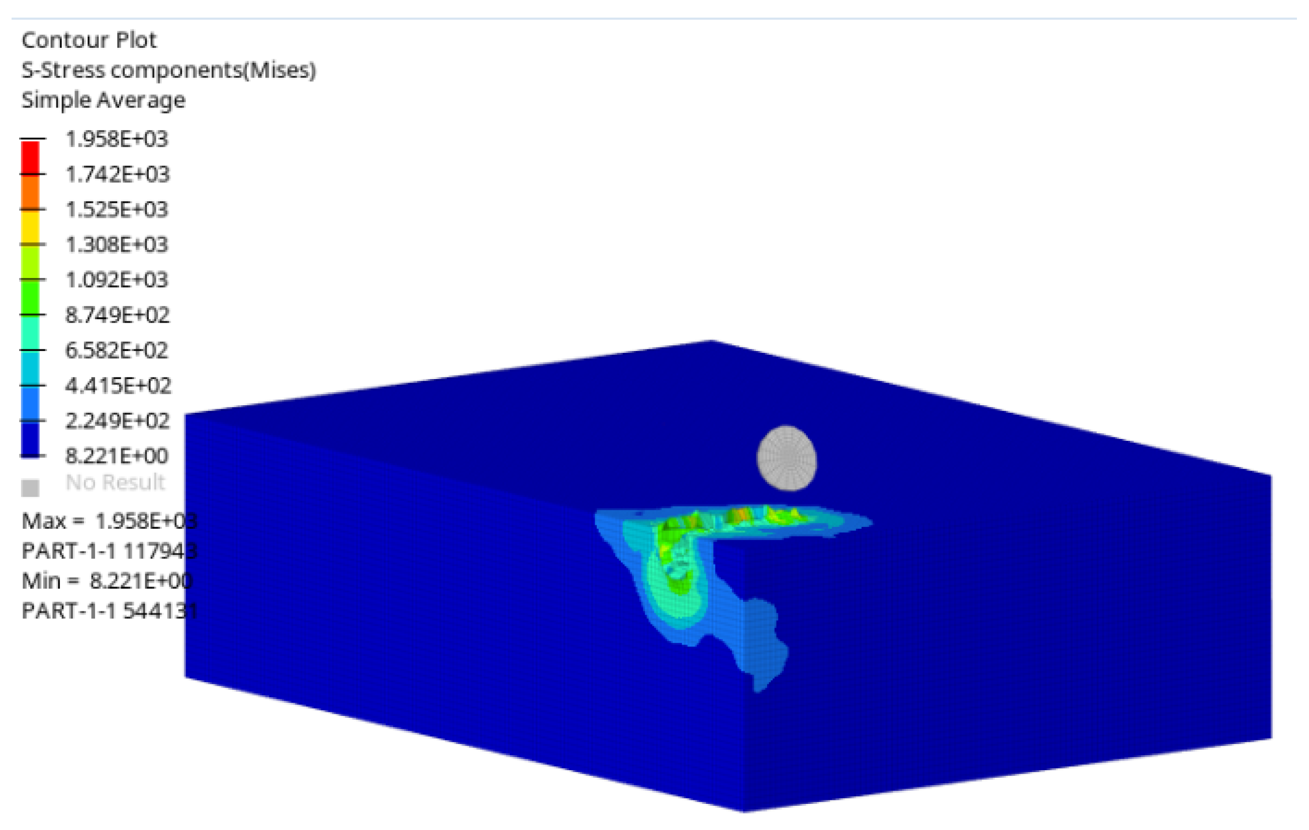
Simulation analysis is then conducted in the ABAQUS 2020 software. For computational efficiency, the tool is simplified by excluding the tool holder and retaining only the tool head. The ball-end mill is modeled as a rigid body, with tool wear effects neglected. The C3D8R element type is employed for discretization, which exhibits reduced susceptibility to shear self-locking under bending loads, thereby demonstrating superior performance in bending-dominated problems. Additionally, this element provides relatively accurate displacement solutions and maintains solution accuracy even under conditions of mesh distortion or deformation. The tool model consists of 544 elements and 694 nodes, with a seed size of 0.1. The workpiece is discretized using C3D8R reduced-integration hexahedral elements, resulting in 560,000 elements and 583,881 nodes. The total number of elements in the global model is 560,544, with a total of 584,575 nodes. Numerical simulations are performed using the ABAQUS explicit dynamic solver, with a computational time of 0.06 s.

The tool is inclined at a 20° angle relative to the workpiece plane. During the milling process, the tool exhibits a composite motion of high-speed rotation and translation. The milling process simulation is shown in Figure 3, and the surface residual stresses obtained under different milling process parameter combinations are shown in

Table 6. Residual stress simulation results.

Serial Number	$\mathit{n}/\mathit{r}\cdot {\mathbf{min}}^{-1}$	${\mathit{f}}_{\mathit{z}}/\mathbf{m}\mathbf{m}\cdot {\mathit{z}}^{-1}$	${\mathit{a}}_{\mathit{p}}/\mathbf{m}\mathbf{m}$	${\mathit{a}}_{\mathit{e}}/\mathbf{m}\mathbf{m}$	$\mathit{\sigma }/\mathbf{Mpa}$
1	8 × 103	0.16	1.25	0.15	−195.8
2	8 × 103	0.20	1.50	0.20	−257.5
3	8 × 103	0.24	1.75	0.25	−316.2
4	8 × 103	0.28	2.00	0.30	−371.4
5	1 × 104	0.16	1.50	0.25	−220.7
6	1 × 104	0.20	1.25	0.30	−452.3
7	1 × 104	0.24	2.00	0.15	−294.2
8	1 × 104	0.28	1.75	0.20	−334.9
9	1.2 × 104	0.16	1.75	0.30	−243.4
10	1.2 × 104	0.20	2.00	0.25	−482.6
11	1.2 × 104	0.24	1.25	0.20	−369.1
12	1.2 × 104	0.28	1.50	0.15	−310.8
13	1.4 × 104	0.16	2.00	0.20	−198.6
14	1.4 × 104	0.20	1.75	0.15	−394.1
15	1.4 × 104	0.24	1.50	0.30	−311.7
16	1.4 × 104	0.28	1.25	0.25	−243.6

.

A multi-factor analysis of the results in Table 6 reveals that the variation regularity of surface residual stress under the influence of four process parameters is as follows: a_p > a_e > f_Z > n. During the milling process of small impellers, residual stress decreases as a_p and a_e decreases, and increases as n and f_Z increases, consistent with the variation regularity of surface residual stress in 7075 aluminum alloy [10], thereby validating the accuracy of the established model. Residual stress σ is also expressed by an exponential function composed of four process parameters, as shown in Equation (12):

$$\sigma =C_2{n}^{b_1}{f_z}^{b_2}{a_p}^{b_3}{a_e}^{b_4}$$

(12)

In Equation (12): C₂ is the coefficient of the workpiece material and milling conditions; $b_1$, $b_2$, $b_3$, $b_4$ are the exponents of each processing parameter. Conversion of both sides of Equation (12) to their logarithmic forms is shown in Equation (13):

$$\mathit{ln}\sigma =\mathit{ln}{C}_2+b_1\mathit{ln}n+b_2\mathit{ln}{f}_z+b_3\mathit{ln}{a}_p+b_4\mathit{ln}{a}_e$$

(13)

Let $y=\mathit{ln}\sigma ,b_0=\mathit{ln}{C}_2,x_1=\mathit{ln}n,x_2=\mathit{ln}{f}_z,x_3=\mathit{ln}{a}_p,x_4=\mathit{ln}{a}_e$, then Equation (13) transforms into Equation (14):

$$y=b_0+b_1{x}_1+b_2{x}_2+b_3{x}_3+b_4{x}_4$$

(14)

In Equation (13), parameters $\mathit{ln}n,\mathit{ln}{f}_z,\mathit{ln}{a}_p \mathrm{and} \mathit{ln}{a}_e$ may all be acquired from the preceding experimental data, while the remaining parameters ($b_0,b_1,b_2,b_3,b_4$) are derived via computational programming using 16 sets of the aforementioned experimental data in MATLAB.

Finally, after multiple iterations using MATLAB program code, the final residual stress prediction model was obtained, as shown in Equation (15):

$$\sigma =-164.7492\cdot n^{-0.0016}\cdot {f_z}^{-211.0374}\cdot {a_p}^{-38.7862}\cdot {a_e}^{-92.8891}$$

(15)

3.5. Optimization of Small Impeller Process Parameters Based on Genetic Algorithms

3.5.1. Genetic Algorithm

A genetic algorithm is an optimization algorithm based on the theory of natural selection and the genetic mechanisms of similar species. First, the parameter space is replaced with an encoded space, and then a fitness function is defined and used as the basis for evaluation. The encoded population serves as the basis for population evolution. The iterative process of genetic algorithms is based on selection and genetic mechanisms, achieving random recombination of superior genes in individual bit strings, so that the newly generated offspring population set is superior to the parent population set [11].

3.5.2. Multi-Objective Optimization Mathematical Model

Through the selection of the above design variables, the determination of constraints, and the establishment of the objective function, a multi-objective optimization mathematical model for small impeller process parameters was obtained, as shown in Equation (16):

$$\left\{\begin{array}{l}X=\left[n,f_z,a_p,a_e\right],X\in R^4\\ \min f(X)=0.5\times 3.1548n^{-0.0001}{f_z}^{-10.452}{a_p}^{0.8599}{a_e}^{-4.6697}\\ +0.5\times (-164.7492)n^{-0.0016}{f_z}^{-211.0374}{a_p}^{-38.7862}{a_e}^{-92.8891}\\ s.t\left\{\begin{array}{l}{n}_{\min }\le n\le n_{\max },8000\le n\le 14000\\ v_{c\min }\le v_c\le v_{c\max },26\le v_c\le 44\\ a_{p\min }\le a_p\le a_{p\max },1.25\le a_p\le 2.00\\ a_{e\min }\le a_e\le a_{e\max },0.15\le a_e\le 0.30\end{array}\right.\end{array}\right.$$

(16)

In Equation (16), n, n_max and n_min denote the machine tool spindle speed, maximum spindle speed, and minimum spindle speed, respectively, with the unit of r/min; v_c, v_cmax, and v_cmin referring to the machining feed rate, maximum allowable feed rate during machining, and minimum allowable feed rate, respectively, with the unit of mm/min; a_p, a_pmax, and a_pmin representing the axial depth of cut in the machining process, maximum allowable axial depth of cut, and minimum allowable axial depth of cut, respectively, with the unit of mm; a_e, a_emax, and a_emin standing for the radial depth of cut in the machining process, maximum allowable radial depth of cut, and minimum allowable radial depth of cut, respectively, with the unit of mm.

With specific parameters in Equation (16) held constant, the remaining parameters were systematically varied and analyzed to examine the effect of their variations on the residual stress induced during the machining process of the small impeller. The resulting functional graphs are presented in Figure 4a–d. The points corresponding to minimum residual stress are selected for optimization, followed by a detailed analysis of the machining parameters of the small impeller.

3.5.3. Process Parameter Optimization Based on Genetic Algorithms

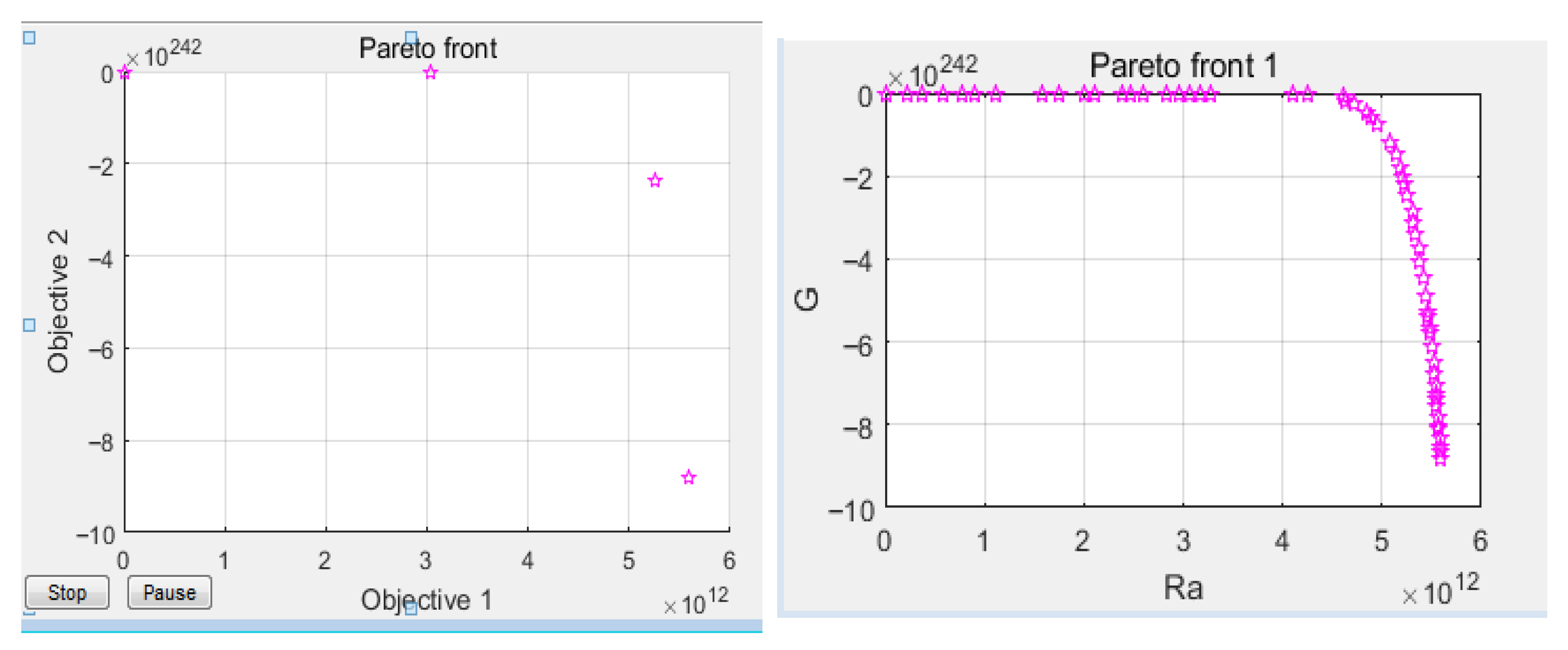
For convenience of calculation, Population Size is set to 200, Crossover Fraction is set to 0.9, Migration Fraction is set to 0.15, and Evolutionary Generations is set to 300 [12]. The results of the program running in MATLAB 2020 are shown in Figure 5.

The optimal parameter combination obtained is shown in Figure 5. Within the range of experimental parameters, the optimal solution obtained by MATLAB genetic algorithms a_p and a_e is close to the minimum value, while n and f_Z take relatively large values, ensuring that surface roughness and residual stress are minimized, thereby improving the surface quality of the small impeller. The corresponding process parameter combination is shown in

Table 7. Optimal combination of process parameters and unoptimized process parameters.

	n/r·min−1	fz/mm·z−1	ap/mm	ae/mm
Unoptimized Process Parameters	8 × 103	0.24	1.75	0.25
Optimized Process Parameters	1.2884 × 104	0.17736	1.2618	0.26551

.

3.5.4. CNC Machining Experimental Verification

The optimized process parameters and CNC machining program were applied to the CNC machining experiment of the small impeller. The experimental machine tool selected is Beijing Jingdiao JDGR200A10SH five-axis machining center. After completing the processing, the experimenter used detection instruments to measure the surface roughness and residual stress of the small impeller.

(1) Verify surface roughness

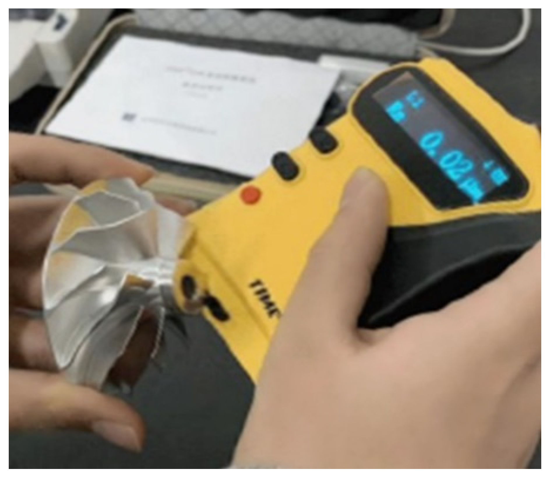
Blades are a critical component in the design and manufacture of small impellers. The surface precision and quality of the blades directly impact the overall mechanical performance of the small impeller [13]. Strict requirements are imposed on the deformation during the blade manufacturing process, particularly regarding surface roughness, which is $Ra\le 3.2 \mathsf{\mu }\mathrm{m}$. As shown in Figure 6, a surface roughness measurement instrument was used to measure the surface roughness of the physical blades of the small impeller before and after optimization of the CNC machining process.

Nine sets of blade surfaces were randomly selected for surface roughness measurement, and the results were compared with those of small impellers processed using unoptimized process parameters. The measurement results are shown in

Table 8. Comparison of surface roughness before and after optimization.

Blade	Ra of Measured Values (μm)									Average Value
unoptimized	1.51	1.82	2.01	1.89	1.96	2.11	1.67	1.84	1.76	1.84
after optimization	0.96	1.47	1.24	1.45	1.10	0.86	1.54	1.03	1.22	1.21

.

According to the measurement results in Table 8, it can be seen that using the optimized process parameters for milling the small impeller reduced the surface roughness by 34.2% and met the processing technical requirements of R_a ≤ 3.2 μm, indicating that the surface quality of the small impeller processed under the optimized process parameters met the standards and was of good quality.

(2) Verification of residual stress

Measurements were taken at three random points on the small impeller blades using an X-350A X-ray stress tester, and the measurement results for the random points on the blades are shown in

Table 9. Random point 1 residual stress measurement results.

$\mathit{\psi }$	0.0°	25.0°	35°	45°
$2^{\theta }p$	138.725°	138.690°	138.737°	138.545°
$\sigma$	−131.2 MPa		error $\Delta \sigma$	±10 MPa

,

Table 10. Random point 2 residual stress measurement results.

$\mathit{\psi }$	0.0°	25.0°	35°	45°
$2^{\theta }p$	137.344°	137.071°	137.176°	137.215°
$\sigma$	−128.4 MPa		error	±10 MPa

and

Table 11. Random point 3 residual stress measurement results.

$\mathit{\psi }$	0.0°	25.0°	35°	45°
$2^{\theta }p$	138.725°	138.686°	138.733°	138.552°
$\sigma$	−129.6 MPa		error	±10 MPa

.

Based on the average measurement results of three random points, the optimized residual stress value $\sigma$ is 129.7, which is 28.6% lower than the pre-optimization value $\sigma$ of 181.6. This indicates that the surface quality of the small impeller processed under the optimized process parameters meets the standards and is of good quality.

After comparing the results before and after testing, it was found that when processing was carried out using the unoptimized process parameters, the small impeller flow channels were extremely narrow, leading to tool breakage, and the surface quality of the processed small impellers did not improve. However, when CNC machining was performed using the optimized process parameters, the CNC machine operated stably during processing, and no tool interference or collisions occurred. The tool’s service life was significantly extended. After parameter optimization, the surface roughness and residual stress of the small impeller were both reduced compared to the values before optimization. This indicates that the optimized process parameters can improve the surface quality of the small impeller.

4. Conclusions

(1)

Focusing on the structural characteristics and processing difficulties of the small impeller, axial cutting depth $a_p$, radial cutting depth $a_e$, spindle speed $n$ and feed per tooth $f_{\mathrm{Z}}$, these four important processing parameters were selected to conduct orthogonal milling experiments on workpieces. By using finite element simulation software, how the milling force changes when each set of process parameters changes can be determined. Then, the data of simulated milling force of each group of machining parameters were analyzed by multi-factor analysis function. Finally, based on the above analysis results, we can obtain the influence of process parameters on the milling force, a prediction model was established based on this to verify the model accuracy.

(2)

Based on the orthogonal test, the surface roughness of the small impeller blades under different process parameters was measured. By parametric fitting, we can obtain the empirical formula of surface roughness. Then, finite element simulation technology was used to build a simplified model of the single blade in the milling process and the residual stress value in blade milling process under different process parameters was simulated by orthogonal test. Finally, the method of parameter fitting was used again to obtain the residual stress empirical formula.

(3)

According to the optimization principle, taking the minimization of surface roughness and the minimization of residual stress as the optimization goals, we can obtain the optimal combination of process parameters by constructing a multi-objective optimization mode of small impeller machining process parameters and using genetic algorithm to optimize the process parameters. On this basis, the numerical control machining experiment of the small impeller was carried out to verify that the optimized process parameters are greatly improved, the surface roughness is reduced by 34.2%, and the residual stress is reduced by 28.6%, and at the same time, the feasibility of the optimization of the process parameters is proved.