Mechanism-Guided and Attention-Enhanced Time-Series Model for Rate of Penetration Prediction in Deep and Ultra-Deep Wells

Abstract

Accurate prediction of the rate of penetration (ROP) in deep and ultra-deep wells remains a major challenge due to complex downhole conditions and limited real-time data. To address the issues of physical inconsistency and weak generalization in conventional da-ta-driven approaches, this study proposes a mechanism-guided and attention-enhanced deep learning framework. In this framework, drilling physical principles such as energy balance are reformulated into differentiable constraint terms and directly incorporated in-to the loss function of deep neural networks, ensuring that model predictions strictly ad-here to drilling physics. Meanwhile, attention mechanisms are integrated to improve feature selection and temporal modeling: for tree-based models, we investigate their implicit attention to key parameters such as weight on bit (WOB) and torque; for sequential models, we design attention-enhanced architectures (e.g., LSTM and GRU) to capture long-term dependencies among drilling parameters. Validation on 49,284 samples from 11 deep and ultra-deep wells in China (depth range: 1226–8639 m) demonstrates that the synergy between mechanism constraints and attention mechanisms substantially improves ROP prediction accuracy. In blind-well tests, the proposed method achieves a mean absolute percentage error (MAPE) of 9.47% and an R² of 0.93, significantly outperforming traditional methods under complex deep-well conditions. This study provides reliable intelligent decision support for optimizing deep and ultra-deep well drilling operations. By improving prediction accuracy and enabling real-time anomaly detection, it enhances operational safety and efficiency while reducing drilling risks. The proposed approach offers high practical value for field applications and supports the intelligent development of the oil and gas industry.

1. Introduction

Accurate prediction of the rate of penetration (ROP) is fundamental to optimizing drilling parameters, enhancing drilling efficiency, and reducing operational costs [1]. As a key performance indicator in drilling operations, ROP is jointly influenced by lithological properties, drilling equipment characteristics, and dynamic operational conditions [2]. Developing a high-fidelity ROP prediction model is therefore essential for real-time drilling optimization and intelligent decision-making in complex well environments [3].

Traditional approaches to ROP prediction have largely relied on physics-based models rooted in drilling mechanics. Classical empirical and semi-theoretical models, such as the Bourgoyne and Young model [4] and Bingham formulations [5], provide useful insights into bit–rock interactions. However, these models are inherently constrained by simplifying assumptions. They often neglect critical uncertainties in real drilling processes, including heterogeneity in rock formations, tool wear, and continuous adjustments of operational parameters [6]. Consequently, their predictive performance tends to deteriorate in deep and ultra-deep wells where downhole conditions are highly variable and nonlinear [7].

Recent advances in drilling monitoring technologies have enabled the collection of large volumes of real-time drilling data, creating new opportunities for data-driven ROP prediction [8]. Machine learning and deep learning techniques are particularly promising, as they can capture complex nonlinear relationships among drilling parameters and adapt to diverse geological and operational conditions [9,10]. In recent years, numerous studies have confirmed the advantages of machine learning and deep learning techniques. For instance, Liu et al. [11] systematically compared multiple regression algorithms for multivariate ROP prediction, demonstrating that Gradient Boosting regression achieved the best performance, with its prediction accuracy positively correlated with training data size and the number of logging features, and validated its effectiveness in adjacent wells. Similarly, Wang et al. [12] proposed a PCA-Informer model that significantly outperformed traditional RNN and LSTM methods in prediction accuracy by combining principal component analysis with the Informer architecture, providing a new solution for actual drilling operations. Furthermore, Allawi et al. [13] applied and compared multiple boosting machine learning models including Gradient Boosting (GBM) and Extreme Gradient Boosting (XGBoost) for ROP prediction in the West Qurna oil field, confirming that these ensemble learning methods can achieve high-precision predictions with low error rates while identifying optimal ranges for 14 key operational parameters to enhance drilling efficiency. Additionally, a 2025 study [14] on a hybrid Gradient Boosting Machine (GBM) model optimized via Bayesian Probability of Improvement algorithm achieved a test R² of 0.773, highlighting the potential of hybrid, optimally tuned machine learning models as robust tools for data-driven ROP prediction. Moreover, Liu et al. [15] developed a dynamic multi-step ROP prediction model by integrating a continuous learning structure with a self-attention mechanism, demonstrating its enhanced capability to capture long-term dependencies within sequential drilling data and achieving over 90% prediction accuracy in field applications, which significantly improves the reliability of long-sequence ROP forecasting. Meanwhile, Tu Bingrui et al. [16] introduced a GRU-Informer model for real-time ROP prediction, where GRU networks capture short-term correlations in drilling parameters and the Informer component handles long-term dependencies, with experimental results showing superior performance over traditional RNNs, LSTMs, and standalone GRU or Informer models. Nevertheless, purely data-driven models often suffer from two critical shortcomings: (i) a lack of physical interpretability, leading to predictions that may contradict known drilling mechanisms [17], and (ii) limited generalization capability when applied to wells with unseen geological settings [18].

To address these challenges, this study proposes a mechanism-guided and attention-enhanced deep learning framework for accurate ROP prediction in deep and ultra-deep wells. In this framework, fundamental drilling physics—such as energy balance principles—are reformulated into differentiable constraint terms and embedded directly into the loss function of deep neural networks, ensuring that predictions remain consistent with drilling mechanisms [19]. In parallel, attention mechanisms are introduced to strengthen feature selection and temporal modeling capabilities, thereby enhancing the model’s ability to capture long-term dependencies among drilling parameters [20]. By synergizing physical constraints with advanced deep learning techniques, the proposed framework bridges the gap between mechanism-based and data-driven approaches, providing both physical interpretability and high predictive accuracy [21].

2. Materials and Methods

2.1. Data Preparation

2.1.1. Data Overview

This study utilizes a comprehensive dataset comprising 49,284 samples from 11 deep and ultra-deep wells in China, with depths ranging from 1226 to 8639 m, all drilled with PDC bits. As shown in

Table 1. Parameters and Boundaries.

Category	Parameters
Engineering	Depth
	Torque
	WOB
	RPM
	SPP
	ROP
	ECD
	Inlet Density
	$\mathrm{F}\mathrm{l}\mathrm{o}\mathrm{w}\mathrm{I}\mathrm{n}$
	Inlet Temperature
	Outlet Temperature
Formation	Formation
Drilling Tools	Bit Size
	Bit Type
	Drill Footage
	Total Area of Water Holes

, the dataset encompasses 16 key features including engineering parameters (e.g., WOB), bit parameters (e.g., bit size), and geological parameters (e.g., formation).

2.1.2. Data Processing Methods

To ensure the quality and reliability of the input data for subsequent modeling, a comprehensive and rigorous data preprocessing pipeline was implemented [22]. The work-flow involved outlier removal, data imputation, feature selection, and data smoothing.

1.

Outlier Removal Based on 3σ Criterion

The first step involved the identification and elimination of anomalous data points that could significantly skew the model’s learning process. The 3σ criterion [23], a common statistical method assuming a normal distribution of data, was employed for this purpose. For each feature, the mean (μ) and standard deviation (σ) were calculated. Any data point lying outside the range of (μ − 3σ, μ + 3σ) was considered an outlier and subsequently removed from the dataset. This process effectively filters out extreme values with a 99.7% confidence interval, thereby enhancing the dataset’s overall robustness.

2.

Data Imputation using K-Nearest Neighbors (KNNs) Algorithm

The removal of outliers and the inherent nature of field data collection inevitably resulted in missing values. To address this issue without introducing significant bias, the K-Nearest Neighbors (KNN) algorithm [24] was utilized for data imputation. This method identifies the K most similar samples (neighbors) to the sample with the missing value, based on the Euclidean distance across other features. The missing value is then imputed as the mean (or median) of that feature from the identified neighbors. Compared to simple mean/median imputation, the KNN algorithm preserves the intrinsic relationships within the dataset, leading to a more accurate and realistic estimation of the missing values.

3.

Data Smoothing with Savitzky–Golay (SG) Filter

Downhole data acquisition is often contaminated with high-frequency noise due to vibrations, sensor malfunctions, and transmission errors. To suppress this noise while preserving the essential trends and patterns of the data, the Savitzky–Golay (SG) [25] smoothing filter was applied [22]. Unlike simple moving average filters that can distort signal peaks, the SG filter works by fitting successive sub-sets of adjacent data points with a low-degree polynomial using the method of linear least squares. This sophisticated approach effectively smooths the data while maintaining the original shape and critical features of the signal, such as relative maxima and minima, which are crucial for accurate ROP modeling.

4.

Feature Selection via Pearson Correlation Analysis

To mitigate multicollinearity and eliminate irrelevant features, thus reducing model complexity and improving generalizability, two-stage feature selection was conducted using Pearson correlation analysis. First, the Pearson correlation coefficient between all pairs of input features was computed. If the absolute correlation coefficient between any two features exceeded 0.9, indicating severe multicollinearity, one of them was removed to prevent redundant information. Second, the absolute correlation coefficient between each remaining feature and the target variable (ROP) was calculated. Features exhibiting an absolute correlation with ROP of less than 0.1 were deemed to have a negligible linear relationship with the target and were subsequently discarded. This process resulted in an optimal subset of features that are both non-redundant and informative for predicting ROP.

2.1.3. Dataset Splitting Strategy

To rigorously evaluate the generalizability and performance of the developed model across different geological formations and depth intervals, a structured dataset splitting strategy was employed. Rather than employing random splitting, which could lead to data leakage and overoptimistic performance estimates, the dataset was partitioned on a well-by-well basis. This approach simulates a realistic operational scenario where the model is trained on historical data from offset wells and subsequently deployed to predict the drilling performance of a new, unseen well.

The dataset comprising 11 deep and ultra-deep wells was divided as follows:

• Training Set (9 wells): Wells labeled X1 through X9 were used for model training. This set provides the model with a broad learning base, encompassing a wide depth range from 1226 m to 8639 m, which includes diverse drilling conditions and geological features.
• Validation Set (1 well): Well Y1 (depth range: 3800–8242 m) was specifically designated as the validation well. This well was used to provide an intermediate assessment of the model’s predictive capability, ensuring that the model was performing well on unseen data before final evaluation.
• Test Set (1 well): Well Z1 (depth range: 4602–7542 m) was designated as the fully blind test well. This well was not used during the training or validation phases and was reserved exclusively for the final, unbiased evaluation of the model’s performance, providing a true measure of its predictive ability on completely unseen data.

The respective depth coverage of each subset is illustrated in Figure 1. This splitting framework ensures that the model’s performance is tested on geographically distinct data, providing a robust and operationally relevant evaluation of its practical utility.

2.2. Applications of the Attention

The integration of attention mechanisms has become a pivotal advancement in ma-chine learning, significantly enhancing model interpretability and predictive performance across diverse domains. These mechanisms can be broadly categorized into two paradigms: implicit and explicit attention. Implicit attention refers to the innate, model-intrinsic ability of certain algorithms to prioritize features or instances through their inherent learning process, without a dedicated architectural component. This is exemplified by tree-based ensemble models like Random Forest, Gradient Boosting Machines (XGBoost, LightGBM, CatBoost), and other boosting variants, which naturally learn and utilize feature importance. In contrast, explicit attention involves a distinct, parameterized module that is deliberately incorporated into a model’s architecture to dynamically compute and apply weighting schemes. This approach is prominently featured in neural network-based sequences models, such as Att-LSTM and Att-GRU, where a dedicated attention layer actively learns to assign context-dependent weights to different parts of the input sequence. This section delves into the foundational principles of both paradigms, elucidating their operational mechanisms and theoretical underpinnings.

2.2.1. Implicit Attention

Implicit attention denotes the intrinsic, often indirect, capability of a machine learning model to focus on the most informative features or samples during its training phase. Unlike its explicit counterpart, this form of attention is not governed by a separate computational submodule but is an emergent property of the model’s core algorithm. In tree-based ensembles, such as Random Forest, XGBoost, LightGBM, and CatBoost, this attentional behavior is manifested through the learning of feature importances.

The principle operates on the premise that features which contribute most significantly to reducing impurity (e.g., Gini impurity or entropy) or minimizing loss across a multitude of trees are deemed more critical. The model, through iterative splitting and boosting, implicitly “pays more attention” to these features by granting them a higher probability of being selected for splits and by relying on them for making pivotal decisions. For instance, in a boosting algorithm, the process of sequentially correcting the errors of previous weak learners inherently directs focus (i.e., attention) towards the most challenging instances to predict, effectively assigning them greater weight in subsequent learning rounds. Thus, the attentional mechanism, while not formally instantiated as a distinct layer, is fundamentally embedded within the model’s learning dynamics and is quantitatively reflected in the computed feature importance scores.

2.2.2. Explicit Attention

Explicit attention refers to a modular, algorithmic component that is consciously de-signed and integrated into a model’s architecture to dynamically compute a set of weights, signifying the relative importance of individual elements within an input. This mechanism allows the model to adaptively focus on the most relevant parts of the input for a given task or context, a process that is fully differentiable and learned end-to-end during training. The core principle involves three key steps: First, a scoring function evaluates the relevance of each element in the input sequence (e.g., hidden states of an RNN) relative to a current context or query. Second, these scores are normalized into a set of attention weights (typically using a softmax function), which sum to one and represent a probability distribution over the input elements. Finally, a context vector is generated as a weighted sum of the input elements, using the computed attention weights. This context vector, which encapsulates a focused view of the input, is then used for downstream pre-diction. This paradigm is powerfully illustrated in models like Att-LSTM and Att-GRU, where a dedicated attention layer is placed atop the recurrent network. Instead of relying solely on the final hidden state to represent the entire sequence, the attention mechanism allows the model to weigh all previous hidden states when generating the output. This explicitly mitigates the information bottleneck problem inherent in standard RNNs and empowers the model to capture long-range dependencies more effectively by directly at-tending to relevant information anywhere in the input sequence, regardless of distance.

2.3. Hybrid Loss Function Formulation

The core contribution of this work is the development of a composite loss function that penalizes deviations from both empirical observations and established physical principles.

2.3.1. Data Loss Term

The data loss component ensures alignment between model predictions and measured field data, where ROP is derived from the inverse of drilling time.

$$L_{\mathrm{d}\mathrm{a}\mathrm{t}\mathrm{a}}={\displaystyle \frac{1}{N}}\sum _{i=1}^N{\left(RO{P}_{\mathrm{p}\mathrm{r}\mathrm{e}\mathrm{d}}^{\left(i\right)}-RO{P}_{\mathrm{r}\mathrm{e}\mathrm{a}\mathrm{l}}^{\left(i\right)}\right)}^2$$

(1)

2.3.2. Physics-Informed Constraints

To guide the neural network towards physically plausible predictions and improve its generalizability, we introduce three physics-based constraint terms derived from simplified models of the drilling process.

• Mechanical Energy Constraint

The rate of penetration is fundamentally linked to the mechanical work done by the drill bit to crush rock. A widely used and simplified model that captures this relationship is the Bingham model [4,5], which expresses ROP as proportional to the work rate per unit area:

$$ROP\propto {\displaystyle \frac{WOB\cdot RPM\cdot BitDiameter}{A_b}}$$

(2)

where $A_b$ is the bit cross-sectional area. For a given bit size, the diameter and area are constant. Therefore, the model can be simplified to the following:

$$ROP=K_1^{\prime }\cdot \left(WOB\cdot RPM\right)$$

(3)

Here, the composite parameter $K_1^{\prime }$ encapsulates the effects of bit design, rock type, and efficiency. Our mechanical energy loss term is designed to penalize significant deviations from this fundamental trend, encouraging the model to learn a relationship where ROP increases with both WOB and RPM. The loss term is formulated as the mean squared error between the predicted ROP, and this simplified physical model is shown below:

$$L_{\mathrm{m}\mathrm{e}\mathrm{c}\mathrm{h}}={\displaystyle \frac{1}{N}}\sum _{i=1}^N{\left(RO{P}_{\mathrm{p}\mathrm{r}\mathrm{e}\mathrm{d}}^{\left(i\right)}-K_1\cdot WO{B}^{\left(i\right)}\cdot {RPM}^{\left(i\right)}\right)}^2$$

(4)

where $K_1$ is a scalable parameter initialized based on typical values and can be optimized during training.

2.

Hydraulic Energy Constraint

Efficient hole cleaning, which removes drilled cuttings from beneath the bit, is critical for achieving high ROP. The hydraulic horsepower at the bit is a key indicator of cleaning efficiency [26,27]. It is proportional to the product of standpipe pressure (SPP) and flow rate (FlowIn):

$$HSI\propto SPP\cdot FlowIn$$

(5)

where HSI is the Hydraulic Horsepower per Square Inch. A well-cleaned bottom hole allows the bit to engage with fresh rock, thereby increasing ROP. Thus, ROP can be expected to have a positive correlation with the hydraulic energy delivered. Our constraint term enforces this positive correlation:

$$L_{\mathrm{h}\mathrm{y}\mathrm{d}}={\displaystyle \frac{1}{N}}\sum _{i=1}^N{\left({ROP}_{\mathrm{p}\mathrm{r}\mathrm{e}\mathrm{d}}^{\left(i\right)}-K_2\cdot {SPP}^{\left(i\right)}\cdot {FlowIn}^{\left(i\right)}\right)}^2$$

(6)

Here, $K_2$ is another scalable parameter that absorbs the conversion constants and efficiencies. This term guides the model to learn that higher hydraulic energy should generally facilitate a faster ROP, all else being equal.

3.

Formation Strength Constraint

The resistance of the formation to drilling is a primary factor controlling ROP. While complex, a first-order principle is that ROP is inversely proportional to rock strength [28]. Direct measurements of in situ rock strength are not available in standard drilling data. However, the Equivalent Circulating Density (ECD) is influenced by the wellbore pressure required to maintain stability, which is itself related to the strength and fracture gradient of the formation. In many drilling models, a higher ECD can indicate a greater pressure confinement on the rock, effectively increasing its “apparent strength” and making it harder to fail, leading to a reduction in ROP [29]. We therefore propose a simplified constraint using ECD as a proxy for the relative changes in formation strength and confinement:

$$L_{\mathrm{f}\mathrm{o}\mathrm{r}\mathrm{m}\mathrm{a}\mathrm{t}\mathrm{i}\mathrm{o}\mathrm{n}}={\displaystyle \frac{1}{N}}\sum _{i=1}^N{\left({ROP}_{\mathrm{p}\mathrm{r}\mathrm{e}\mathrm{d}}^{\left(i\right)}-{\displaystyle \frac{K_3}{{ECD}^{\left(i\right)}}}\right)}^2$$

(7)

This term penalizes predictions where ROP increases with ECD, which is physically counter-intuitive, and instead encourages the inverse relationship observed in field operations.

4.

Composite Loss Integration

The individual constraint losses are synthesized through a weighted combination:

$$L_{physics}=\alpha \cdot L_{mech}+\beta \cdot L_{hyd}+\gamma \cdot L_{formation}$$

(8)

The weighting coefficients α, β, γ, and λ in Equations (5) and (6) are not pre-defined as fixed hyperparameters. Instead, they are implemented as trainable parameters, initialized to 1.0 and optimized concurrently with the network’s weights during the training process. Similarly, the coefficients K1, K2, and K3 within the physics-based constraints are also treated as trainable parameters of the model, rather than fixed constants. This data-adaptive approach allows the model to autonomously determine the optimal balance between the data fidelity term and the various physics-based constraints, leading to a more robust and generalizable solution.

2.3.3. Loss Function and Optimization Objective

The optimization approach aims to refine ROP predictions by balancing data accuracy with physical plausibility. This is achieved through a composite loss function that combines a standard data-fitting error term with a physics-based regularizer. The physics component incorporates essential drilling principles related to mechanical energy, hydraulic efficiency, and formation strength, ensuring the model’s outputs are not only statistically accurate but also consistent with established domain knowledge.

The complete optimization objective is then defined as follows:

$$L_{total}=L_{data}+\lambda \cdot L_{physics}$$

(9)

2.4. Model Selection and Development

2.4.1. Tree-Based Models

Tree-based ensemble models are a cornerstone of modern machine learning, leveraging the combined predictive power of multiple decision trees to achieve robust and accurate outcomes. A conceptual structure of such an ensemble is illustrated in Figure 2. Despite sharing the foundational principle of aggregating tree outputs, these models diverge in their approaches to tree construction, aggregation, and optimization, resulting in distinct performance characteristics, computational efficiencies, and suitability for diverse data types. By integrating numerous “weak” learners (individual decision trees), these methods create a “strong” learner that mitigates the overfitting risks associated with single, overly complex trees. The progression from Random Forest to advanced gradient boosting frameworks, such as XGBoost, LightGBM, and CatBoost, reflects ongoing advancements in scalability, accuracy, and adaptability to large-scale and complex datasets.

1.

Random Forest

Random Forest employs bagging (Bootstrap Aggregating) to construct an ensemble of decision trees, each trained on a randomly sampled subset of the data with replacement and a random subset of features. This dual randomness in data and feature selection ensures that individual trees are decorrelated, capturing diverse patterns within the data. Final predictions are generated by averaging outputs (for regression) or taking a majority vote (for classification) across all trees. This approach significantly reduces variance and overfitting compared to a single decision tree, making Random Forest a robust, user-friendly algorithm, particularly effective for high-dimensional datasets [30]. Its ability to provide feature importance scores further enhances its interpretability, making it a staple in applications requiring reliable predictions without extensive tuning [31].

2.

Extreme Gradient Boosting (XGBoost)

XGBoost [32] is an advanced gradient boosting framework that builds trees sequentially, with each tree correcting the residual errors of its predecessors. Its key strengths lie in its optimization techniques and regularization strategies. By employing a second-order Taylor expansion of the loss function, XGBoost achieves more precise tree construction than standard gradient descent methods. Additionally, it incorporates L1 (Lasso) and L2 (Ridge) regularization terms in its objective function to control model complexity and prevent overfitting. This combination of sophisticated optimization and regularization enables XGBoost to deliver exceptional accuracy, making it a preferred choice in machine learning competitions and real-world applications, despite its computational intensity [33]. Its scalability has been widely validated across diverse domains, including structured data prediction tasks.

3.

Light Gradient Boosting Machine (LightGBM)

Developed by Microsoft, LightGBM [34] is a gradient boosting framework optimized for efficiency and scalability on large datasets. Its innovative features include Gradient-based One-Side Sampling (GOSS) and Exclusive Feature Bundling (EFB). GOSS prioritizes instances with large gradients—those harder to predict—while randomly sampling instances with smaller gradients, thereby focusing computational resources on the most informative data points. EFB reduces dimensionality by bundling mutually exclusive features into a single feature, enhancing efficiency. Unlike level-wise tree growth, LightGBM adopts a leaf-wise approach, selecting the leaf with the maximum loss reduction for expansion, which often accelerates convergence and improves accuracy. However, careful parameter tuning is required to prevent overfitting, particularly on smaller datasets. LightGBM’s efficiency makes it ideal for large-scale industrial applications.

4.

Categorical Boosting (CatBoost)

CatBoost [35] is a gradient boosting algorithm designed to handle categorical features effectively, addressing a common challenge in real-world datasets. Its standout feature is its advanced treatment of categorical variables, using target statistics to compute expected target values for each category while incorporating a prior to mitigate overfitting. This approach avoids target leakage and reduces the need for extensive feature engineering. Additionally, CatBoost employs Ordered Boosting, a novel gradient-boosting scheme that addresses prediction shift issues inherent in traditional boosting, enhancing model robustness and generalizability, especially for datasets with rich categorical features. Its performance has been rigorously validated in applications involving heterogeneous data, making it a versatile tool for complex predictive tasks.

2.4.2. Time-Series Models

Time-series data, prevalent in applications such as drilling operations, exhibit complex sequential dependencies that challenge conventional modeling techniques. Standard Recurrent Neural Networks (RNNs) often fail to capture long-range dependencies due to the vanishing gradient problem, which impedes learning from temporally distant events [36]. To address this, advanced gated RNN architectures, namely Long Short-Term Memory (LSTM) and Gated Recurrent Unit (GRU), were developed. These models employ gating mechanisms to regulate information flow, enabling selective retention and updating of information over extended sequences. This capability makes them ideal for modeling intricate drilling processes, where historical parameters like weight-on-bit or torque influence future outcomes, such as the Rate of Penetration (ROP). While both LSTM and GRU aim to capture temporal dynamics, they differ in architectural complexity and gating strategies, offering distinct trade-offs in performance and computational efficiency.

• Long Short-Term Memory (LSTM)

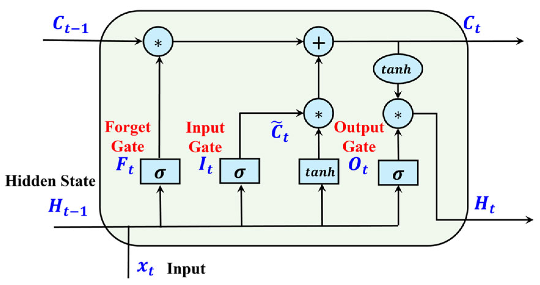
The Long Short-Term Memory (LSTM) network addresses the vanishing gradient problem through a memory cell regulated by three specialized gates: the input gate, forget gate, and output gate [37]. The architecture of an LSTM unit, depicting the interplay of these gates, is shown in Figure 3. The forget gate determines which prior information to discard from the cell state, while the input gate controls the integration of new information from the current input. The output gate dictates which parts of the updated cell state are passed as the hidden state to the next timestep. By maintaining a separate cell state and using additive updates, LSTMs effectively preserve critical information over long sequences, making them robust for modeling complex sequential patterns, such as those in drilling operations where long-term dependencies are critical [38]. This architectural design provides fine-grained control over memory dynamics, enabling LSTMs to excel in tasks requiring the retention of long-term temporal relationships.

The following equations define the operations at a single time step t:

Forget Gate (F_t): This gate decides what information to discard from the previous cell state C_t−1. It takes the current input x_t and the previous hidden state H_t−1 as input and outputs a vector of values between 0 (completely forget) and 1 (completely retain).

$$F_t=\sigma \left(W_f\cdot \left[H_{t-1},x_t\right]+b_f\right)$$

(10)

Input Gate (I_t): This gate controls the extent to which new information is stored in the cell state. It also uses the current input and previous hidden state.

$$I_t=\sigma \left(W_i\cdot \left[H_{t-1},X_t\right]+b_i\right)$$

(11)

Candidate Cell State ($\tilde{C}$_t): A vector of new candidate values, created from the current input, that could be added to the cell state.

$${\tilde{C}}_t=\mathrm{t}\mathrm{a}\mathrm{n}\mathrm{h}\left(W_C\cdot \left[H_{t-1},X_t\right]+b_C\right)$$

(12)

Cell State Update (C_t): The new cell state C_t is computed by first element-wise multiplying the previous cell state C_t−1 by the forget gate’s output (to “forget” irrelevant information) and then adding the element-wise product of the input gate and the candidate state (to “remember” new relevant information).

$$C_t=F_t\odot C_{t-1}+I_t\odot {\tilde{C}}_t$$

(13)

Output Gate (O_t): This gate determines which parts of the updated cell state C_t will be output as the hidden state H_t.

$$O_t=\sigma \left(W_o\cdot \left[H_{t-1},X_t\right]+b_o\right)$$

(14)

Hidden State (H_t): The final hidden state for the current time step is computed by passing the updated cell state through a tanh activation function and then filtering it with the output gate.

$$H_t=O_t\odot \mathrm{t}\mathrm{a}\mathrm{n}\mathrm{h}\left(C_t\right)$$

(15)

2.

Gated Recurrent Unit (GRU)

The Gated Recurrent Unit (GRU) offers a streamlined alternative to the LSTM, designed to achieve comparable performance with reduced computational complexity [39]. By merging the cell state and hidden state and utilizing only two gates—the update gate and the reset gate—GRUs simplify the architecture. The streamlined structure of the GRU cell is illustrated in Figure 4. The update gate balances the retention of past information with the incorporation of new input, while the reset gate determines how much of the previous hidden state to ignore when computing the candidate activation. This parsimonious design results in fewer trainable parameters, leading to faster training times and lower computational demands compared to LSTMs, often with minimal compromise in predictive accuracy. GRUs are particularly advantageous in resource-constrained environments or with smaller datasets, making them suitable for real-time time-series applications, such as monitoring drilling processes [40].

The key innovation of the Gated Recurrent Unit (GRU) is its update gate (Z_t), which elegantly combines the separate forget and input gates of an LSTM into a single, unified mechanism. This gate directly regulates the interpolation between the previous hidden state and a new candidate state, allowing the model to dynamically control information retention and renewal within a more streamlined architecture. This elegant design is captured by its core state update equation:

$$H_t=\left(1-Z_t\right)\odot H_{t-1}+Z_t\odot {\tilde{H}}_t$$

(16)

2.5. Evaluation Indicators

2.5.1. Mean Absolute Error (MAE)

The Mean Absolute Error (MAE) is a widely adopted metric for assessing the accuracy of predictive models, particularly in applications like Rate of Penetration (ROP) forecasting in drilling operations [22]. It computes the average of the absolute differences between predicted and actual values, offering a straightforward and interpretable measure of prediction error. Unlike the Mean Squared Error (MSE), MAE assigns equal weight to all errors, making it less sensitive to outliers and thus more robust in datasets with extreme values [41]. A lower MAE indicates that the model’s predictions are, on average, closer to the true values, providing a reliable gauge of overall performance.

$$MAE={\displaystyle \frac{1}{n}}\sum _{i=1}^n\left|RO{P}_{\mathrm{r}\mathrm{e}\mathrm{a}\mathrm{l}}^{\left(i\right)}-RO{P}_{\mathrm{p}\mathrm{r}\mathrm{e}\mathrm{d}}^{\left(i\right)}\right|$$

(17)

2.5.2. Coefficient of Determination (R²)

The Coefficient of Determination (R²) quantifies the proportion of variance in the observed data that is explained by the model’s predictions, serving as a critical indicator of goodness-of-fit. It evaluates how effectively the predicted values capture the variability of the actual data around its mean, making it particularly valuable for assessing model performance in regression tasks like ROP prediction. An R² value approaching 1 indicates that the model explains a substantial portion of the target variable’s variance, reflecting strong predictive capability, while a lower R² suggests a weaker fit [42]. This metric is widely used to compare the explanatory power of different models across diverse applications.

$$R^2=1-{\displaystyle \frac{\sum _{i=1}^n{\left(RO{P}_{\mathrm{r}\mathrm{e}\mathrm{a}\mathrm{l}}^{\left(i\right)}-RO{P}_{\mathrm{p}\mathrm{r}\mathrm{e}\mathrm{d}}^{\left(i\right)}\right)}^2}{\sum _{i=1}^n{\left(RO{P}_{\mathrm{r}\mathrm{e}\mathrm{a}\mathrm{l}}^{\left(i\right)}-{\overline{ROP}}_{\mathrm{r}\mathrm{e}\mathrm{a}\mathrm{l}}\right)}^2}}$$

(18)

2.5.3. Mean Absolute Percentage Error (MAPE)

The Mean Absolute Percentage Error (MAPE) measures the average magnitude of prediction errors as a percentage of the actual observed values, providing a scale-independent metric for evaluating forecast accuracy. This makes MAPE particularly useful in practical applications, such as ROP prediction, where understanding relative errors facilitates operational decision-making. By expressing errors as percentages, MAPE offers an intuitive interpretation of model performance, especially when comparing predictions across datasets with different scales [43]. A lower MAPE value signifies higher predictive accuracy, making it a valuable tool for assessing model reliability in real-world scenarios.

$$MAPE={\displaystyle \frac{100\mathrm{\%}}{n}}\sum _{i=1}^n\left|{\displaystyle \frac{RO{P}_{\mathrm{r}\mathrm{e}\mathrm{a}\mathrm{l}}^{\left(i\right)}-RO{P}_{\mathrm{p}\mathrm{r}\mathrm{e}\mathrm{d}}^{\left(i\right)}}{RO{P}_{\mathrm{r}\mathrm{e}\mathrm{a}\mathrm{l}}^{\left(i\right)}}}\right|$$

(19)

3. Results

3.1. Data Processing

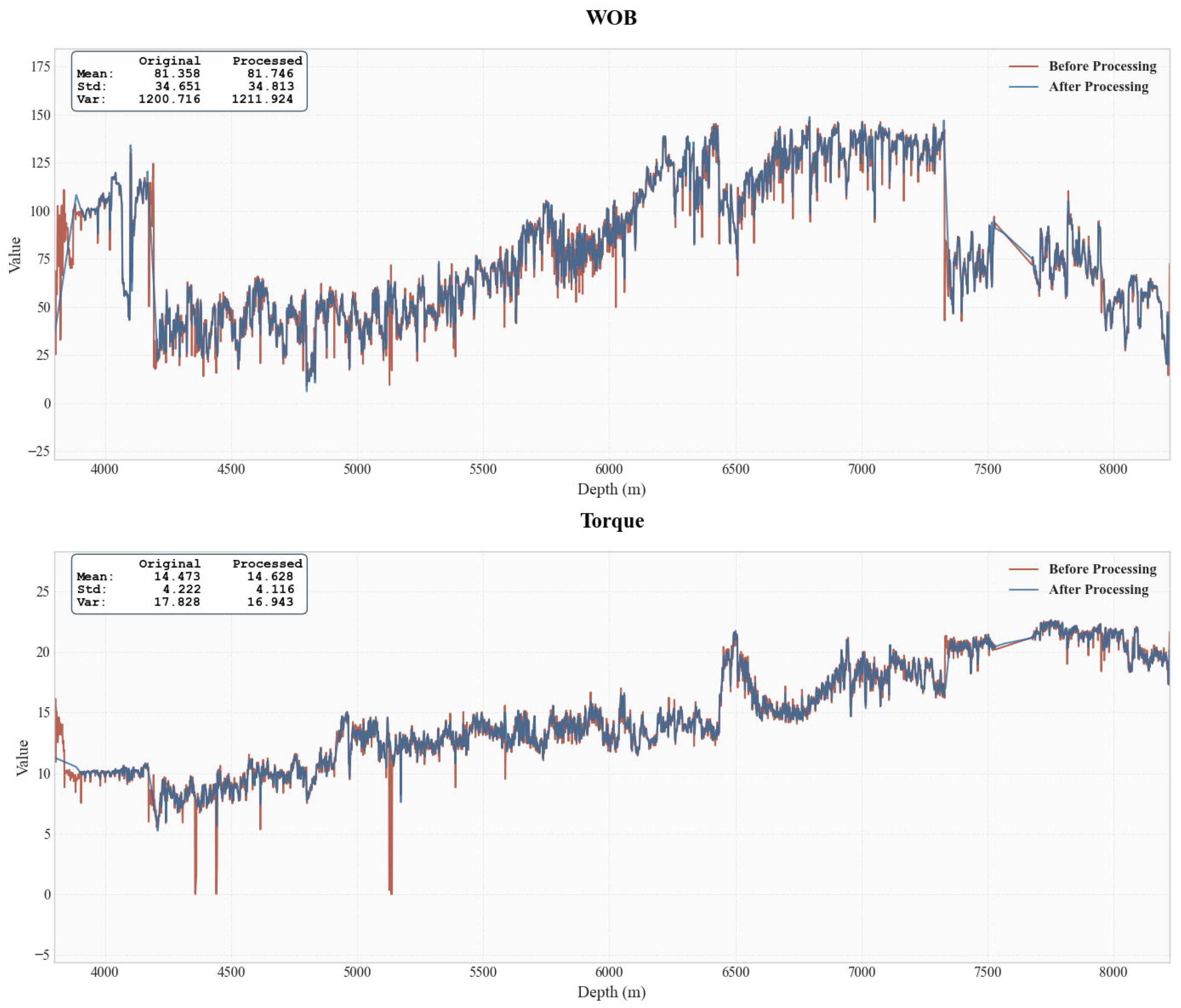
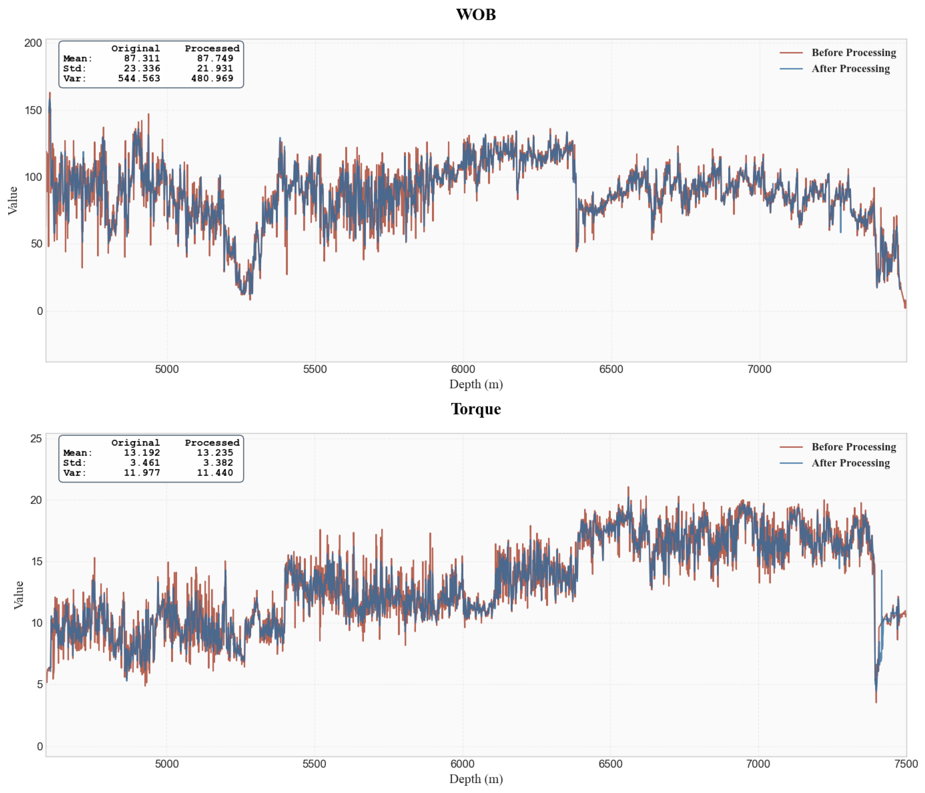
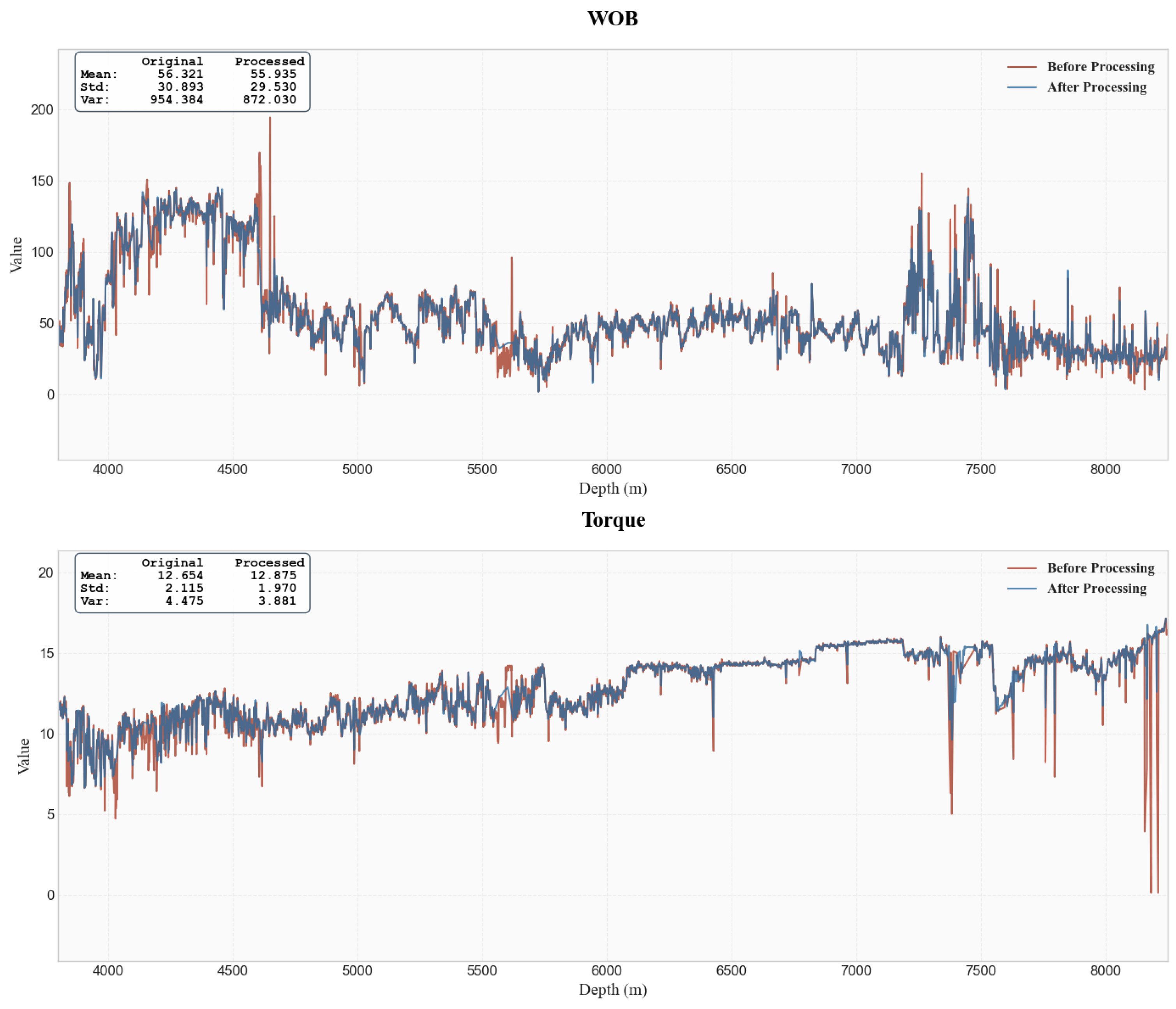
Following the comprehensive preprocessing pipeline outlined in Section 2, a high-quality dataset was obtained for model development and evaluation, with comparative diagrams illustrating the data before and after processing for three representative wells (the training well X2 in Figure 5, the test well Y1 in Figure 6, and the validation well Z1 in Figure 7). The final processed dataset consists of 38,426 training samples derived from offset wells, covering a extensive depth range from 1226 to 8639 m (a span of 7413 m). This broad coverage ensures the model is exposed to a wide variety of drilling conditions and geological formations. The validation set contains 3640 samples from well Y1, spanning a depth interval of 2940.8 m (4602.0–7542.8 m). The test set, from well Z1, covers a depth range of 4442.0 m (3800.0–8242.0 m), providing a robust challenge for assessing model generalizability.

The quality of the processed data was quantitatively assessed by comparing key statistical metrics—namely the mean, variance, and standard deviation—of critical parameters before and after processing. A representative analysis was conducted on wells X2 (training), Y1 (validation), and Z1 (test). The results demonstrated a marked improvement in data quality. The application of the 3σ outlier removal and SG filtering significantly reduced anomalous spikes and high-frequency noise, which was reflected in stabilized variance and standard deviation values. Furthermore, the KNN imputation ensured data completeness without introducing substantial bias, preserving the original statistical distribution of the dataset. This rigorous preprocessing procedure resulted in a clean, consistent, and reliable dataset, forming a solid foundation for subsequent model training and evaluation.

3.2. Ablation Study

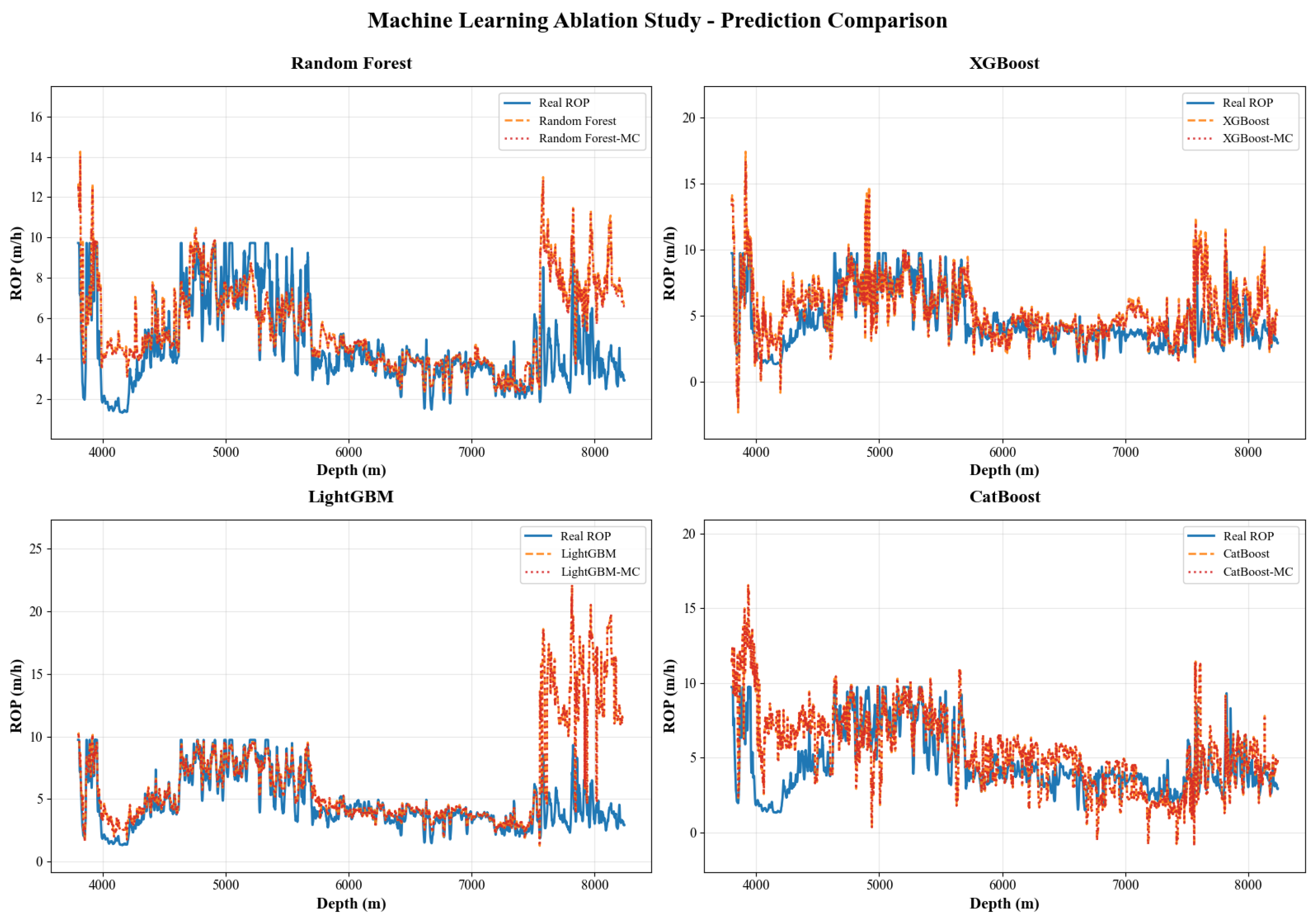
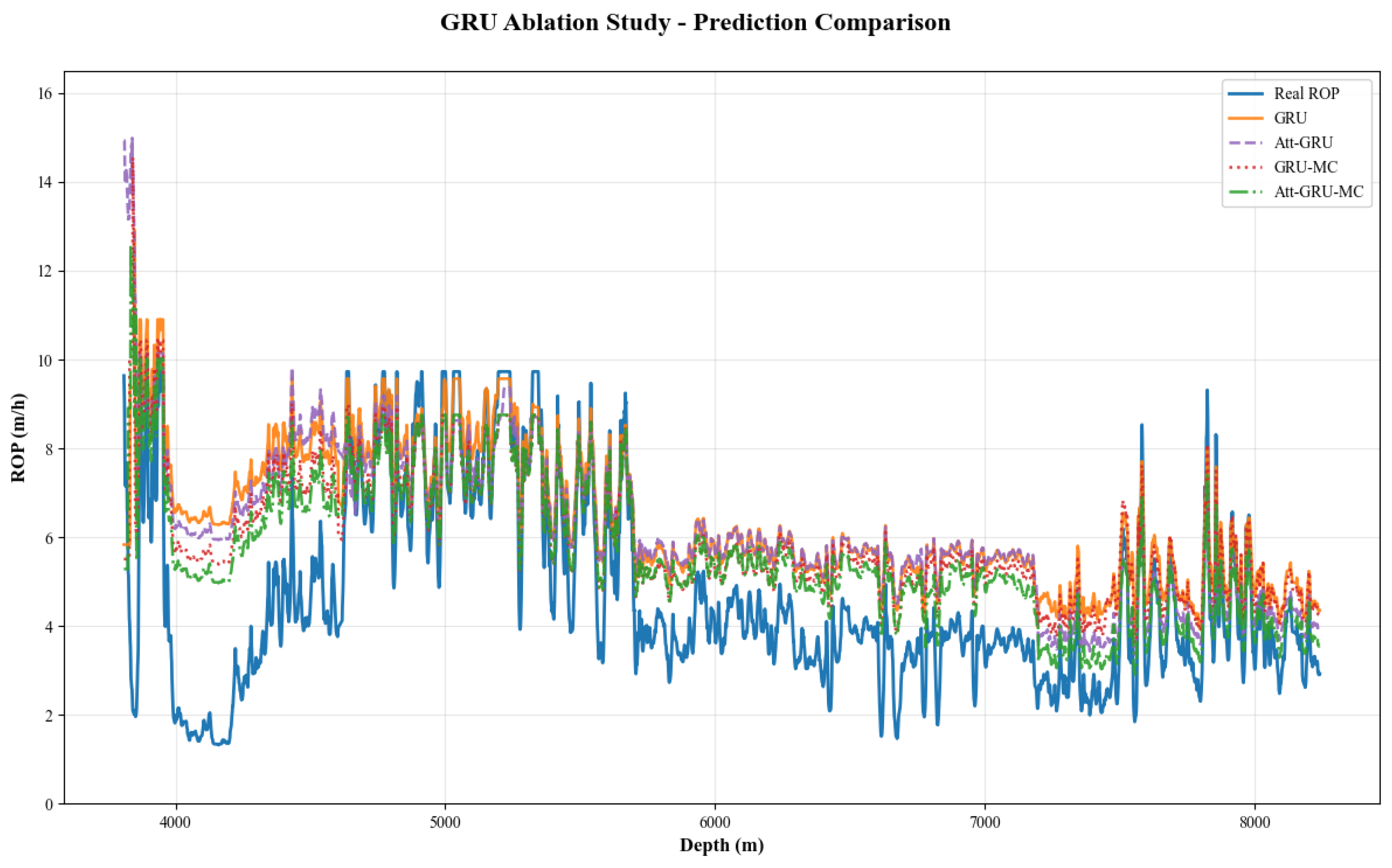
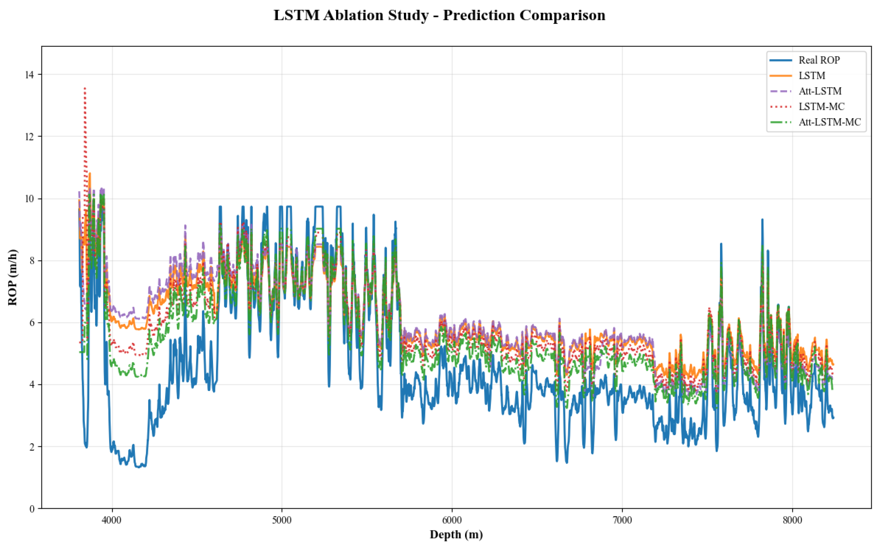
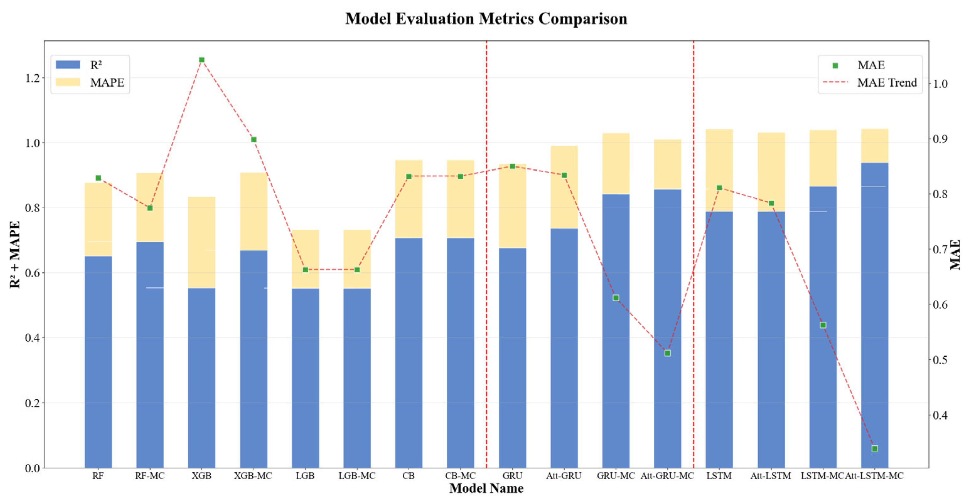
To systematically validate the effectiveness of the proposed approach, we incorporated a physics-based constraint loss function into the training process of all machine learning models (e.g., Random Forest, XGBoost) and deep learning models (e.g., LSTM, GRU). Experimental results demonstrate that the introduction of physical constraints significantly improved the prediction accuracy of all models, reducing the mean absolute error (MAE) and root mean square error (RMSE), while increasing the coefficient of determination (R²). The performance comparison of different machine learning methods under physical constraints is shown in Figure 8. This confirms that guidance by physical principles enhances the generalization capability of the models. Furthermore, on the basis of the physical constraints, we integrated attention mechanisms (Att-LSTM, Att-GRU) into the deep learning models to enhance their ability to capture long-term dependencies in drilling time-series data. The comparative results of the GRU-based variants are presented in Figure 9, while the LSTM-based variants are compared in Figure 10. The comparative results clearly showed that the deep learning models combined with attention mechanisms achieved the best performance on the test well, with the predicted curves exhibiting the highest agreement with the true values and a further reduction in error. A comprehensive comparison of all evaluation indicators across different methods is summarized in Figure 11.

4. Discussion

This study demonstrates significant achievements in the field of drilling parameter prediction by integrating mechanistic constraints (MCs) with attention mechanisms, exhibiting high theoretical and practical engineering value. It not only proves that physics-guided machine learning models (e.g., Att-LSTM-MCs) significantly outperform purely data-driven models and traditional machine learning methods in predictive accuracy, but more importantly, greatly enhances the physical plausibility and decision interpretability of the model. The visualization of attention weights allows the model to “emulate” the decision-making processes of experienced engineers, clearly revealing the dynamic importance of key parameters (such as WOB and torque) during different drilling phases. Meanwhile, the physical constraints effectively prevent predictions that violate physical principles, ensuring the model’s robustness and generalization capability under extreme operating conditions. This paradigm of integrating domain knowledge with deep learning provides an effective solution to the long-standing challenges of “black-box nature” and reliability in engineering applications, playing a crucial role in enabling safe and efficient intelligent drilling optimization.

4.1. Analysis of Attention Mechanism

The integration of attention mechanisms has yielded substantial improvements in both predictive accuracy and model interpretability, as evidenced by the comprehensive performance metrics. Among the baseline models without attention mechanisms, GRU-MCs and LSTM-MCs already demonstrated competitive performance with MAPE values of 12.97% and 13.54%, and R² scores of 0.84 and 0.88, respectively. However, the incorporation of attention mechanisms resulted in remarkable enhancements across all evaluation metrics. The Att-LSTM-MCs model emerged as the top performer, achieving a MAPE of 9.47%, an R² of 0.93, along with the lowest RMSE (1.85) and MAE (1.47) among all models. This represents a relative improvement of approximately 30% in MAPE and 5% in R² compared to its non-attention counterpart.

The superior performance of attention-enhanced models can be attributed to their ability to dynamically focus on the most relevant temporal features and drilling parameters during different operational phases. Unlike standard recurrent networks that treat all time steps equally, the attention mechanism enables the model to assign varying im-portance weights to different elements in the input sequence. This capability is particularly valuable in drilling operations where the significance of parameters such as weight-on-bit, torque, and hydraulic measurements varies substantially throughout the drilling process. The attention weights effectively serve as an intrinsic feature selection mechanism, allowing the model to prioritize information that is most predictive of ROP changes while filtering out noisy or irrelevant inputs.

Visualization of the attention weights revealed insightful patterns in how the model processes drilling data. During periods of formation transitions or changing drilling conditions, the attention mechanism consistently allocated higher weights to mechanical parameters such as WOB and torque. Conversely, during stable drilling phases, hydraulic parameters and historical ROP values received greater emphasis. This adaptive behavior demonstrates that the model learns physically meaningful relationships without explicit instruction, effectively mimicking the decision-making process of experienced drilling engineers. The attention mechanism not only enhances predictive performance but also pro-vides valuable insights into the relative importance of different parameters under varying downhole conditions, thereby serving as a window into the model’s decision-making process and significantly improving model interpretability [21].

4.2. Analysis of Physics-Based Constraints

The incorporation of physics-based constraints (MCs) has fundamentally enhanced the physical plausibility and generalization capability of all models in the study. The mechanistic constraints, derived from fundamental drilling energy principles, served as a regularizing influence that guided the models toward physically realistic solutions. This is particularly evident in the consistent performance improvement across all model architectures when compared to their purely data-driven counterparts. The constraints effectively prevented physically impossible predictions that sometimes occur in conventional machine learning models, especially in regions with sparse training data or extreme drilling conditions.

The impact of mechanistic constraints is most pronounced in their effect on model generalization. The deep learning models with mechanistic constraints (LSTM-MCs and GRU-MCs) achieved R² values of 0.88 and 0.84, respectively, significantly outperforming most tree-based models. While CatBoost-MCs showed a relatively high R² of 0.76, its elevated MAPE (17.44%) and MAE (2.28) indicated systematic prediction biases that were substantially reduced in the constrained deep learning models. This demonstrates that the physics-based constraints effectively anchor the models in established drilling principles while maintaining the flexibility to learn complex patterns from data. The constraints act as a form of domain knowledge injection, reducing the hypothesis space that the models need to explore during training and thereby decreasing the risk of overfitting.

The synergistic effect between mechanistic constraints and attention mechanisms is particularly noteworthy. The Att-LSTM-MCs model achieved the best overall performance with a MAPE of 9.47% and R² of 0.93, representing the optimal integration of physical knowledge and data-driven learning. This combination allows the model to leverage the strengths of both approaches: the attention mechanism identifies the most relevant features and temporal dependencies, while the physical constraints ensure that the predictions remain within physically plausible bounds. The constraints also enhance model robustness in challenging drilling environments, as evidenced by the consistent performance across different well conditions. This hybrid approach represents a significant advancement over traditional methods, providing both high accuracy and physical consistency, which is essential for real-world drilling optimization applications where safety and reliability are paramount concerns. The mechanistic constraints essentially serve as a physics-based regularizer, ensuring that the models not only perform well statistically but also operate in accordance with established drilling principles, making them more trust-worthy for critical decision-making in field operations.

4.3. Future Work

Although the proposed physics-informed attention-based model has demonstrated promising results in predicting rate of penetration (ROP), several avenues remain open for further investigation to enhance its applicability and performance. Future research will first focus on exploring more advanced attention mechanisms, such as multi-head attention or transformer-based architectures, to better capture complex temporal dependencies and interactions among multivariate drilling parameters. Building on this, a deeper analysis of the attention weights themselves, particularly through visualization techniques like heatmaps across depth, will be undertaken to quantitatively interpret how the model shifts its focus between parameters (e.g., WOB/RPM vs. hydraulics) during formation transitions, thereby enhancing the model’s interpretability and our understanding of its decision-making process.

Additionally, efforts will be made to integrate more data sources, including logging-while-drilling (LWD) measurements, real-time downhole vibrations, and geomechanical properties, to enrich the input feature space and improve model generalization under varying geological conditions.

Furthermore, a critical area for future work is the rigorous assessment of how specific physics-based constraints, such as our mechanical energy constraint utilizing RPM, quantitatively alter the model’s physical plausibility beyond aggregate performance metrics. This involves detailed analysis of model behavior under specific operational regimes (e.g., high RPM, low torque, or distinct lithologies) to demonstrate enhanced generalization and physical consistency, which will be a focal point of our subsequent research.

Another critical direction involves advancing the model towards real-time field deployment. This will require developing lightweight and computationally efficient versions suitable for edge computing devices, enabling high-frequency inference with low latency—essential for closed-loop drilling optimization. Furthermore, future work will emphasize uncertainty quantification through Bayesian deep learning approaches to provide probabilistic predictions and confidence intervals, thereby enhancing decision-making reliability in high-risk drilling operations.

Lastly, extending the hybrid modeling framework to other drilling optimization objectives, such as tool wear prediction and anomaly detection, represents a promising research direction. Such efforts would contribute to building a more comprehensive and trustworthy AI-assisted drilling system, bridging the gap between data-driven intelligence and domain-specific physical principles.

5. Conclusions

This study presents a comprehensive and novel framework that integrates physics-based constraints and attention mechanisms for predicting the Rate of Penetration (ROP) in complex drilling environments, particularly in deep and ultra-deep wells. The pro-posed methodology is designed to overcome key limitations of conventional purely da-ta-driven approaches, which often produce physically implausible results and lack interpretability, especially when extrapolating to unseen geological conditions. By incorporating domain knowledge derived from drilling mechanics—expressed through mechanistically grounded loss terms—and enhancing temporal feature learning via attention mechanisms, this hybrid approach ensures that predictions are both accurate and physically consistent.

The core design of this study revolves around a dual-strategy architecture. First, physics-based constraints are embedded directly into the learning objective function, formulated using Mean Squared Error (MSE) terms that penalize deviations from established energy-based principles—mechanical, hydraulic, and formation strength relationships. This mechanism not only regularizes the model but also injects foundational drilling knowledge, enabling reliable generalization beyond training data. Second, attention mechanisms are integrated into deep learning models (such as Att-LSTM and Att-GRU), allowing the network to dynamically prioritize informative features and time steps, thereby improving both predictive performance and operational interpretability.

Experimental validation across multiple machine learning and deep learning models confirms the effectiveness of the proposed framework. The combined model (Att-LSTM with physical constraints) achieved a remarkable MAPE of 9.47% and an R² of 0.93 on challenging blind-test wells, significantly outperforming standalone data-driven models. Analysis of attention weights provided actionable insights into the relative importance of drilling parameters under different downhole conditions, offering a window into model decision-making that is valuable for real-time drilling optimization.

Furthermore, this study offers important implications for ROP prediction in deep and ultra-deep wells. The integration of physical principles mitigates the common issue of model overfitting using high-dimensional and noisy drilling data, which is especially critical in extreme drilling environments where data scarcity and unpredictability are major concerns. The attention mechanism’s ability to highlight critical features—such as weight-on-bit and torque during formation transitions—provides drillers with interpretable feedback that can support on-the-fly decision-making.

This work establishes a new paradigm for hybrid modeling in drilling optimization, one that successfully balances data-driven learning with physical principles. It provides a robust foundation for the next generation of intelligent drilling systems, contributing to enhanced efficiency, safety, and cost-effectiveness in hydrocarbon exploration. The framework’s ability to deliver accurate, physically consistent, and interpretable predictions makes it particularly suitable for real-time drilling advisory systems and automated optimization platforms, marking a significant step forward in the digital transformation of oil and gas drilling operations.

References

1. Li, G.; Song, X.; Zhu, Z.; Tian, S.; Sheng, M. Research progress and the prospect of intelligent drilling and completion technologies. Pet. Drill. Technol. 2023, 51, 35–47. [Google Scholar]
2. Bourgoyne, A.T.; Millheim, K.K.; Chenevert, M.E.; Young, F.S. Applied Drilling Engineering; Society of Petroleum Engineers: Richardson, TX, USA, 1986. [Google Scholar]
3. Eren, T.; Ozbayoglu, M.E. Real time optimization of drilling parameters during drilling operations. In Proceedings of the SPE Oil and Gas India Conference and Exhibition? Mumbai, India, 20–22 January 2010; p. SPE-129126-MS. [Google Scholar]
4. Bourgoyne, A.T., Jr.; Young, F., Jr. A multiple regression approach to optimal drilling and abnormal pressure detection. Soc. Pet. Eng. J. 1974, 14, 371–384. [Google Scholar] [CrossRef]
5. Bingham, M.G. A New Approach to Interpreting—Rock Drillability; The Petroleum Publishing Co.: Tulsa, OK, USA, 1965. [Google Scholar]
6. Dupriest, F.E.; Koederitz, W.L. Maximizing drill rates with real-time surveillance of mechanical specific energy. In Proceedings of the SPE/IADC Drilling Conference and Exhibition, Amsterdam, The Netherlands, 23–25 February 2005; p. SPE-92194-MS. [Google Scholar]
7. Soares, C.; Gray, K. Real-time predictive capabilities of analytical and machine learning rate of penetration (ROP) models. J. Pet. Sci. Eng. 2019, 172, 934–959. [Google Scholar] [CrossRef]
8. Noshi, C.I.; Schubert, J.J. The role of machine learning in drilling operations; a review. In Proceedings of the SPE Eastern Regional Meeting, Pittsburgh, PA, USA, 7–11 October 2018; p. D043S005R006. [Google Scholar]
9. Hegde, C.; Gray, K. Use of machine learning and data analytics to increase drilling efficiency for nearby wells. J. Nat. Gas Sci. Eng. 2017, 40, 327–335. [Google Scholar] [CrossRef]
10. Singh, K.; Yalamarty, S.S.; Kamyab, M.; Cheatham, C. Cloud-based ROP prediction and optimization in real-time using supervised machine learning. In Proceedings of the Unconventional Resources Technology Conference, Denver, CO, USA, 22–24 July 2019; pp. 3067–3078. [Google Scholar]
11. Liu, W.; Fu, J.; Tang, C.; Huang, X.; Sun, T. Real-time prediction of multivariate ROP (rate of penetration) based on machine learning regression algorithms: Algorithm comparison, model evaluation and parameter analysis. Energy Explor. Exploit. 2023, 41, 1779–1801. [Google Scholar] [CrossRef]
12. Wang, Y.; Lou, Y.; Lin, Y.; Cai, Q.; Zhu, L. ROP Prediction Method Based on PCA—Informer Modeling. ACS Omega 2024, 9, 23822–23831. [Google Scholar] [CrossRef]
13. Allawi, R.H.; Al-Mudhafar, W.J.; Abbas, M.A.; Wood, D.A. Leveraging Boosting Machine Learning for Drilling Rate of Penetration (ROP) Prediction Based on Drilling and Petrophysical Parameters. Artif. Intell. Geosci. 2025, 6, 100121. [Google Scholar] [CrossRef]
14. Hao, J.; Xu, H.; Peng, Z.; Cao, Z. An online adaptive ROP prediction model using GBDT and Bayesian Optimization algorithm in drilling. Geoenergy Sci. Eng. 2025, 246, 213596. [Google Scholar] [CrossRef]
15. Liu, Y.; Zhang, F.; Yang, S.; Cao, J. Self-attention mechanism for dynamic multi-step ROP prediction under continuous learning structure. Geoenergy Sci. Eng. 2023, 229, 212083. [Google Scholar] [CrossRef]
16. Tu, B.; Bai, K.; Zhan, C.; Zhang, W. Real-time prediction of ROP based on GRU-Informer. Sci. Rep. 2024, 14, 2133. [Google Scholar] [CrossRef] [PubMed]
17. Huang, Z.; Zhu, L.; Wang, C.; Zhang, C.; Li, Q.; Jia, Y.; Wang, L. Intelligent Prediction of Rate of Penetration Using Mechanism-Data Fusion and Transfer Learning. Processes 2024, 12, 2133. [Google Scholar] [CrossRef]
18. Wang, J.; Li, C.; Cheng, P.; Yu, J.; Cheng, C.; Ozbayoglu, E.; Baldino, S. Data integration enabling advanced machine learning ROP predictions and its applications. In Proceedings of the Offshore Technology Conference, Houston, TX, USA, 6–9 May 2024; p. D041S049R003. [Google Scholar]
19. Raissi, M.; Perdikaris, P.; Karniadakis, G.E. Physics-informed neural networks: A deep learning framework for solving forward and inverse problems involving nonlinear partial differential equations. J. Comput. Phys. 2019, 378, 686–707. [Google Scholar] [CrossRef]
20. Vaswani, A.; Shazeer, N.; Parmar, N.; Uszkoreit, J.; Jones, L.; Gomez, A.N.; Kaiser, Ł.; Polosukhin, I. Attention is all you need. Adv. Neural Inf. Process. Syst. 2017, 30, 6000–6010. [Google Scholar]
21. Barbosa, L.F.F.M.; Nascimento, A.; Mathias, M.H.; de Carvalho, J.A. Machine learning methods applied to drilling rate of penetration prediction and optimization—A review. J. Pet. Sci. Eng. 2019, 183, 106332. [Google Scholar] [CrossRef]
22. Peng, C.; Pang, J.; Fu, J.; Cao, Q.; Zhang, J.; Li, Q.; Deng, Z.; Yang, Y.; Yu, Z.; Zheng, D. Predicting Rate of Penetration in Ultra-deep Wells Based on Deep Learning Method. Arab. J. Sci. Eng. 2023, 48, 16753–16768. [Google Scholar] [CrossRef]
23. Barnett, V.; Lewis, T. Outliers in Statistical Data; Wiley: New York, NY, USA, 1994; Volume 3. [Google Scholar]
24. Troyanskaya, O.; Cantor, M.; Sherlock, G.; Brown, P.; Hastie, T.; Tibshirani, R.; Botstein, D.; Altman, R.B. Missing value estimation methods for DNA microarrays. Bioinformatics 2001, 17, 520–525. [Google Scholar] [CrossRef]
25. Savitzky, A.; Golay, M.J. Smoothing and differentiation of data by simplified least squares procedures. Anal. Chem. 1964, 36, 1627–1639. [Google Scholar] [CrossRef]
26. Kendall, H.; Goins, W., Jr. Design and operation of jet-bit programs for maximum hydraulic horsepower, impact force or jet velocity. Trans. AIME 1960, 219, 238–250. [Google Scholar] [CrossRef]
27. Maidla, E.; Ohara, S. Field verification of drilling models and computerized selection off drill bit, WOB, and drillstring rotation. SPE Drill. Eng. 1991, 6, 189–195. [Google Scholar] [CrossRef]
28. Warren, T. Penetration-rate performance of roller-cone bits. SPE Drill. Eng. 1987, 2, 9–18. [Google Scholar] [CrossRef]
29. Schuh, F. The critical buckling force and stresses for pipe in inclined curved boreholes. In Proceedings of the SPE/IADC Drilling Conference and Exhibition, Amsterdam, The Netherlands, 5–7 March 1991; p. SPE-21942-MS. [Google Scholar]
30. Breiman, L. Random forests. Mach. Learn. 2001, 45, 5–32. [Google Scholar] [CrossRef]
31. Biau, G.; Scornet, E. A random forest guided tour. Test 2016, 25, 197–227. [Google Scholar] [CrossRef]
32. Chen, T.; Guestrin, C. Xgboost: A scalable tree boosting system. In Proceedings of the 22nd ACM SIGKDD International Conference on Knowledge Discovery and Data Mining, San Francisco, CA, USA, 13–17 August 2016; pp. 785–794. [Google Scholar]
33. Friedman, J.H. Stochastic gradient boosting. Comput. Stat. Data Anal. 2002, 38, 367–378. [Google Scholar] [CrossRef]
34. Ke, G.; Meng, Q.; Finley, T.; Wang, T.; Chen, W.; Ma, W.; Ye, Q.; Liu, T.-Y. Lightgbm: A highly efficient gradient boosting decision tree. Adv. Neural Inf. Process. Syst. 2017, 30, 3149–3157. [Google Scholar]
35. Prokhorenkova, L.; Gusev, G.; Vorobev, A.; Dorogush, A.V.; Gulin, A. CatBoost: Unbiased boosting with categorical features. Adv. Neural Inf. Process. Syst. 2018, 31, 6639–6649. [Google Scholar]
36. Hochreiter, S.; Schmidhuber, J. Long short-term memory. Neural Comput. 1997, 9, 1735–1780. [Google Scholar] [CrossRef]
37. Greff, K.; Srivastava, R.K.; Koutník, J.; Steunebrink, B.R.; Schmidhuber, J. LSTM: A search space odyssey. IEEE Trans. Neural Netw. Learn. Syst. 2016, 28, 2222–2232. [Google Scholar] [CrossRef]
38. Graves, A.; Schmidhuber, J. Framewise phoneme classification with bidirectional LSTM and other neural network architectures. Neural Netw. 2005, 18, 602–610. [Google Scholar] [CrossRef]
39. Cho, K.; Van Merriënboer, B.; Gulcehre, C.; Bahdanau, D.; Bougares, F.; Schwenk, H.; Bengio, Y. Learning phrase representations using RNN encoder-decoder for statistical machine translation. arXiv 2014, arXiv:1406.1078. [Google Scholar] [CrossRef]
40. Chung, J.; Gulcehre, C.; Cho, K.; Bengio, Y. Empirical evaluation of gated recurrent neural networks on sequence modeling. arXiv 2014, arXiv:1412.3555. [Google Scholar] [CrossRef]
41. Willmott, C.J.; Matsuura, K. Advantages of the mean absolute error (MAE) over the root mean square error (RMSE) in assessing average model performance. Clim. Res. 2005, 30, 79–82. [Google Scholar] [CrossRef]
42. Draper, N. Applied Regression Analysis; McGraw-Hill. Inc.: Columbus, OH, USA, 1998. [Google Scholar]
43. De Myttenaere, A.; Golden, B.; Le Grand, B.; Rossi, F. Mean absolute percentage error for regression models. Neurocomputing 2016, 192, 38–48. [Google Scholar] [CrossRef]
Figure 1. Well depth distribution.
Processes 13 03433 g001
Figure 2. Tree-Based Ensemble Models.
Processes 13 03433 g002
Figure 3. The Architecture of the LSTM Model. The ‘*’ symbol denotes element-wise multiplication, and the ‘+’ symbol denotes element-wise addition.
Processes 13 03433 g003
Figure 4. The Architecture of the GRU Model. The ‘*’ symbol denotes element-wise multiplication, and the ‘+’ symbol denotes element-wise addition.
Processes 13 03433 g004
Figure 5. Comparison of Data Before and After Preprocessing for Test Well X2.
Processes 13 03433 g005
Figure 6. Comparison of Data Before and After Preprocessing for Test Well Y1.
Processes 13 03433 g006
Figure 7. Comparison of Data Before and After Preprocessing for Test Well Z1.
Processes 13 03433 g007
Figure 8. Performance Comparison of Machine Learning Models.
Processes 13 03433 g008
Figure 9. Performance Comparison of GRU-based Models.
Processes 13 03433 g009
Figure 10. Performance Comparison of LSTM-based Models.
Processes 13 03433 g010
Figure 11. Comprehensive Comparison of Evaluation Metrics.
Processes 13 03433 g011