A Multi-Source Data-Driven Fracturing Pressure Prediction Model

Abstract

Accurate prediction of fracturing pressure is critical for operational safety and fracturing efficiency in unconventional reservoirs. Traditional physics-based models and existing deep learning architectures often struggle to capture the intense fluctuations and complex temporal dependencies observed in actual fracturing operations. To address these challenges, this paper proposes a multi-source data-driven fracturing pressure prediction model, a model integrating TCN-BiLSTM-Attention Mechanism (Temporal Convolutional Network, Bidirectional Long Short-Term Memory, Attention Mechanism), and introduces a feature selection mechanism for fracture pressure prediction. This model employs TCN to extract multi-scale local fluctuation features, BiLSTM to capture long-term dependencies, and Attention to adaptively adjust feature weights. A two-stage feature selection strategy combining correlation analysis and ablation experiments effectively eliminates redundant features and enhances model robustness. Field data from the Sichuan Basin were used for model validation. Results demonstrate that our method significantly outperforms baseline models (LSTM, BiLSTM, and TCN-BiLSTM) in mean absolute error (MAE), root mean square error (RMSE), and coefficient of determination (R²), particularly under high-fluctuation conditions. When integrated with slope reversal analysis, it achieves sand blockage warnings up to 41 s in advance, offering substantial potential for real-time decision support in fracturing operations.

1. Introduction

Hydraulic fracturing is one of the key technologies for unconventional oil and gas development [1]. Among numerous parameters, fracturing pressure serves as a core indicator for real-time operational control and sand control/screenout prevention [2]. Accurate pressure prediction not only enhances operational safety but also improves fracturing efficiency. Consequently, fracturing pressure prediction has remained a research hotspot, with many scholars attempting to predict fracturing pressure through physical models. Examples include the classic two-dimensional geometric models PKN and KGD [3,4], as well as the near-wellbore branching/coupling model [5]. However, in actual operations, fracturing pressure often exhibits sudden fluctuations due to stage transitions and changes in fluid properties. These fluctuations are difficult to capture using traditional physical models. In response, with rapid advances in computing, deep learning (DL) has emerged as an effective approach for tackling complex problems and real-time computations [6,7]. It can process large datasets and capture hidden relationships within data sequences [8]. Consequently, DL has gradually found applications in the petroleum industry, such as in drilling rate prediction [9,10], wellbore stability [11,12], lithology prediction [13], and production forecasting [14,15]. These studies not only validate the effectiveness of DL in complex data analysis but also introduce new perspectives and methodologies for fracture pressure prediction.

In recent years, recognizing the periodic nature of fracturing pressure variations, researchers have applied time series forecasting models to fracturing pressure prediction studies. Examples include Deep Recurrent Neural Networks (DRNN), coupled autoregressive integrated moving average (ARIMA) models, locally weighted linear regression (LWLR), and gated recurrent units (GRU) [16,17,18,19]. However, these models excel at capturing long-term dependencies while underperforming in responding to local sudden changes. Consequently, researchers have proposed ensemble models such as convolutional neural networks (CNN)-LSTM, BiLSTM-Attention and other related models [20,21], which outperform single models in overall accuracy. Despite encouraging results, these approaches primarily focus on fitting global trends and often struggle to capture short-term fluctuations triggered by operational switching. Such local errors tend to accumulate and amplify over time, ultimately compromising overall prediction accuracy and peak/inflection reconstruction capabilities [22,23]. Furthermore, redundant features in raw fracturing data undermine model robustness. Additionally, the original fracturing operation data exhibits both multi-scale local abrupt changes and gradual trends, along with highly correlated/redundant features and noise. This can compromise the model’s robustness and generalization capability.

To overcome these limitations, this study proposes a multi-source data-driven fracturing pressure prediction model with integrated feature selection for fracture pressure prediction. Specifically, TCN employs causal and dilated convolutions to expand the receptive field without substantially increasing parameters, robustly capturing multi-scale local fluctuations and abrupt changes. It is particularly sensitive to short-term, sharp variations in pressure curves—such as transient responses triggered by fine-tuning of proppant volume fraction or pump rate. Concurrently, the residual structure enhances gradient stability, BiLSTM models long-term dependencies, and Attention enables adaptive weight adjustment for feature contributions. Simultaneously, by combining two-stage feature selection—correlation analysis followed by ablation experiments—we first “explicitly” eliminate redundancy and then “implicitly” suppress it, thereby jointly enhancing robustness and interpretability. Field validation in the Sichuan Basin demonstrates that when integrated with the slope reversal method, this model can issue sand blockage warnings 41 s earlier than manual operators, highlighting its significant engineering utility.

2. Methods

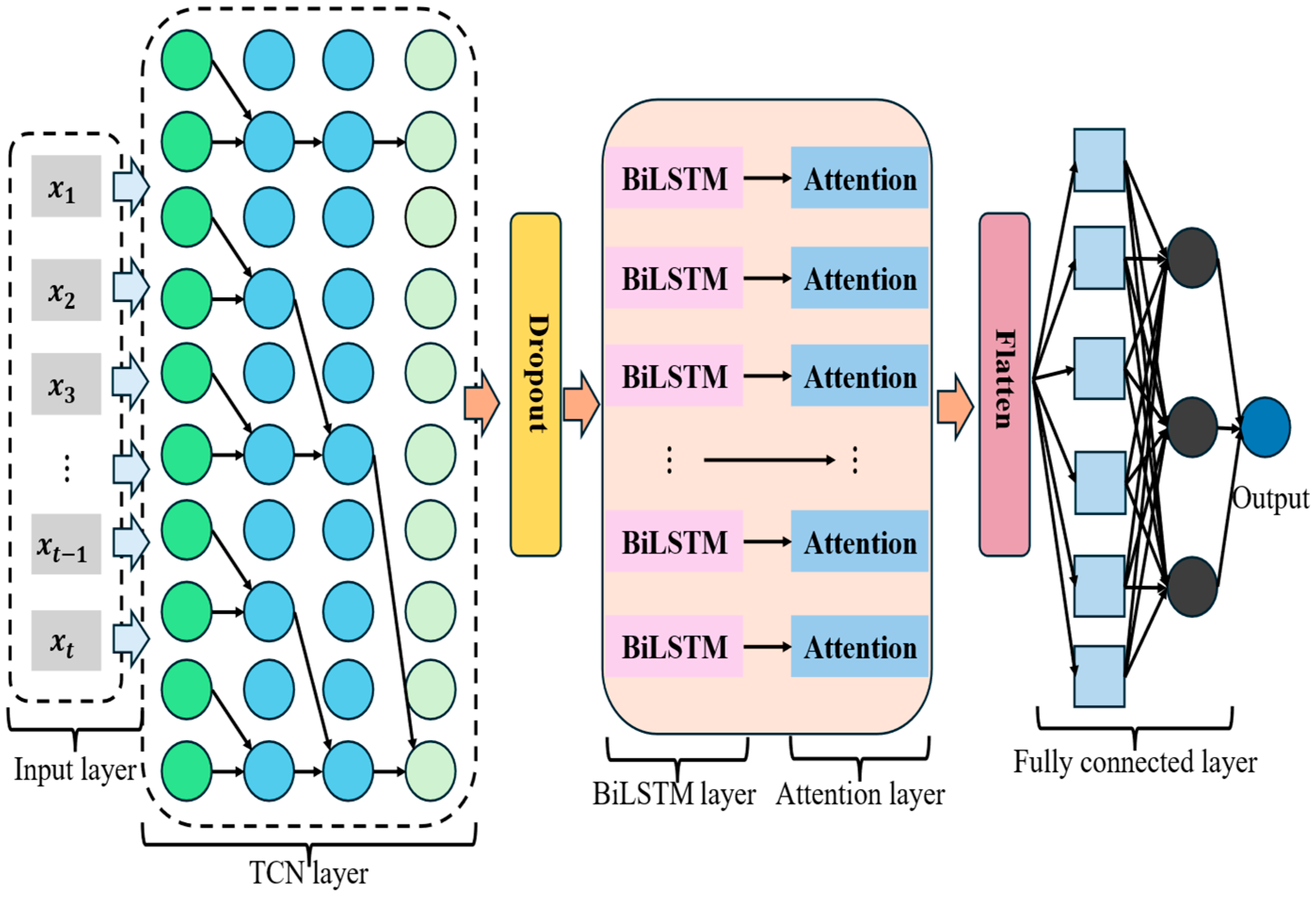
The framework structure of TCN-BiLSTM-Attention is shown as Figure 1, aiming to predict fracturing pressure during the fracturing operation. This model takes engineering parameters from the fracturing process as input to forecast variations in fracturing pressure. It comprises three submodules: TCN, BiLSTM, and Attention. TCN captures temporal patterns within the fracturing engineering parameter data. Simultaneously, BiLSTM captures long-term dependencies by processing both forward and backward contextual information within the time series. Subsequently, the Attention module processes the BiLSTM output to learn long-term sequential features. Finally, a dense layer maps key features into a one-dimensional space for the result output.

2.1. TCN Model

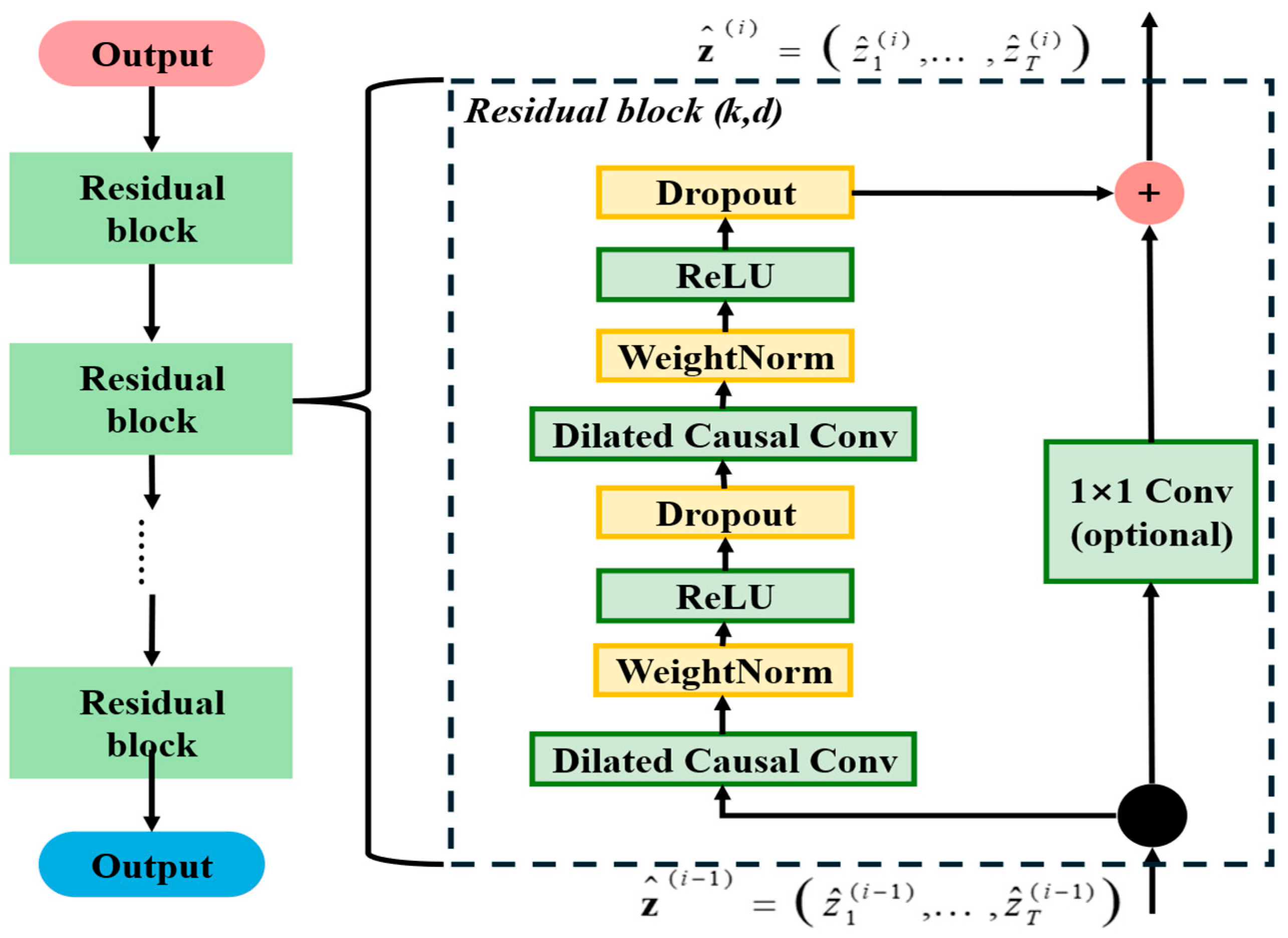
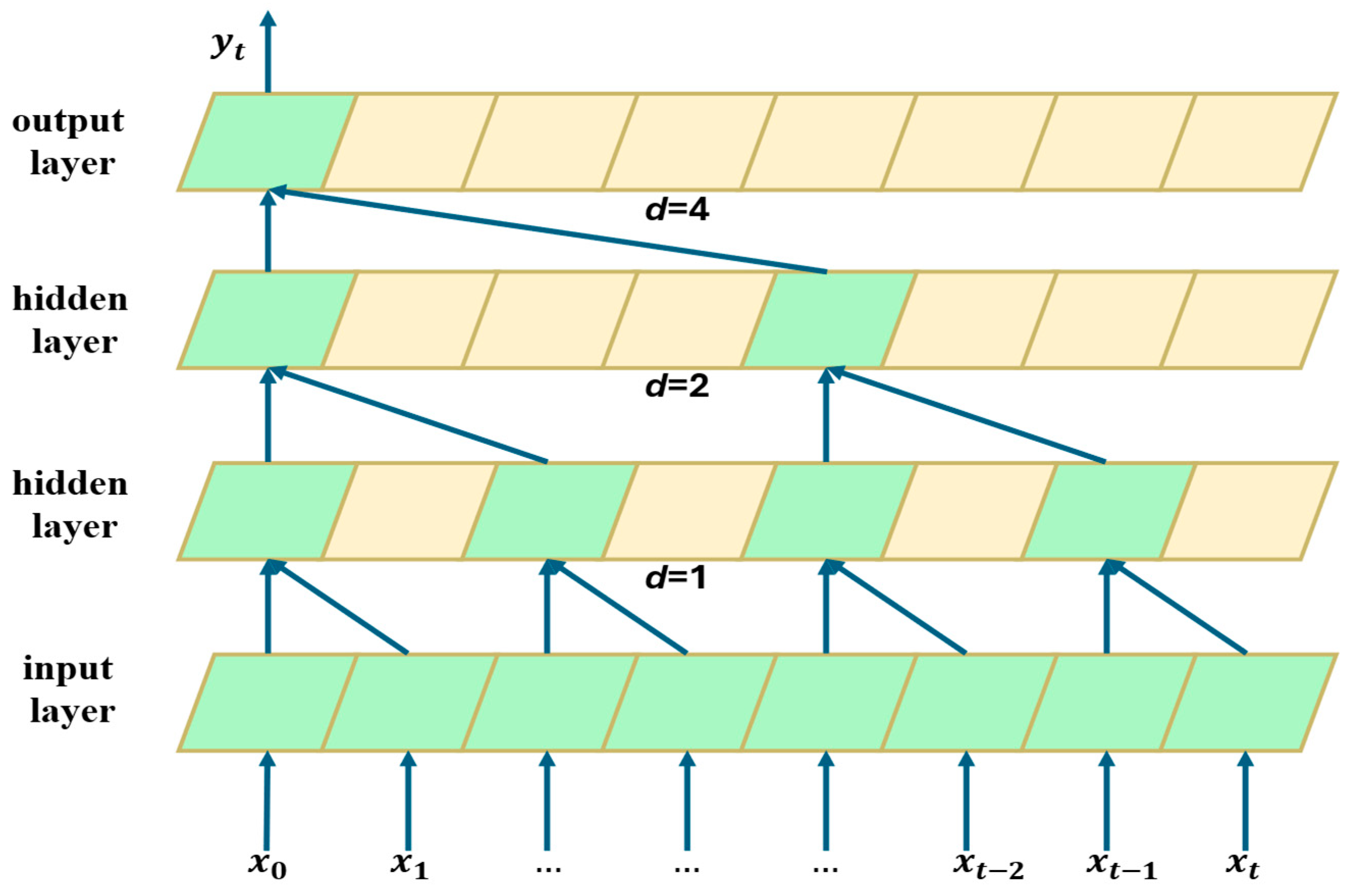
The TCN is an underlying architecture specifically designed for time series forecasting, built upon improvements to the CNN framework structure [24]. This study employs TCN to capture relevant features of local trend changes in data during the fracturing process. TCN consists of three key components—causal convolutions, dilated convolutions, and residual connections [25]. TCNs with kernel sizes of 2 and dilation factors of 1, 2, and 4 exhibit the dilated causal convolution structure shown in Figure 2. The TCN incorporates a residual structure comprising dilated causal convolutions, weight normalization, rectified linear unit (ReLU) activations, and a residual layer, as illustrated in Figure 3. Relevant TCN computational formulas can be found in [26].

2.2. BiLSTM Model

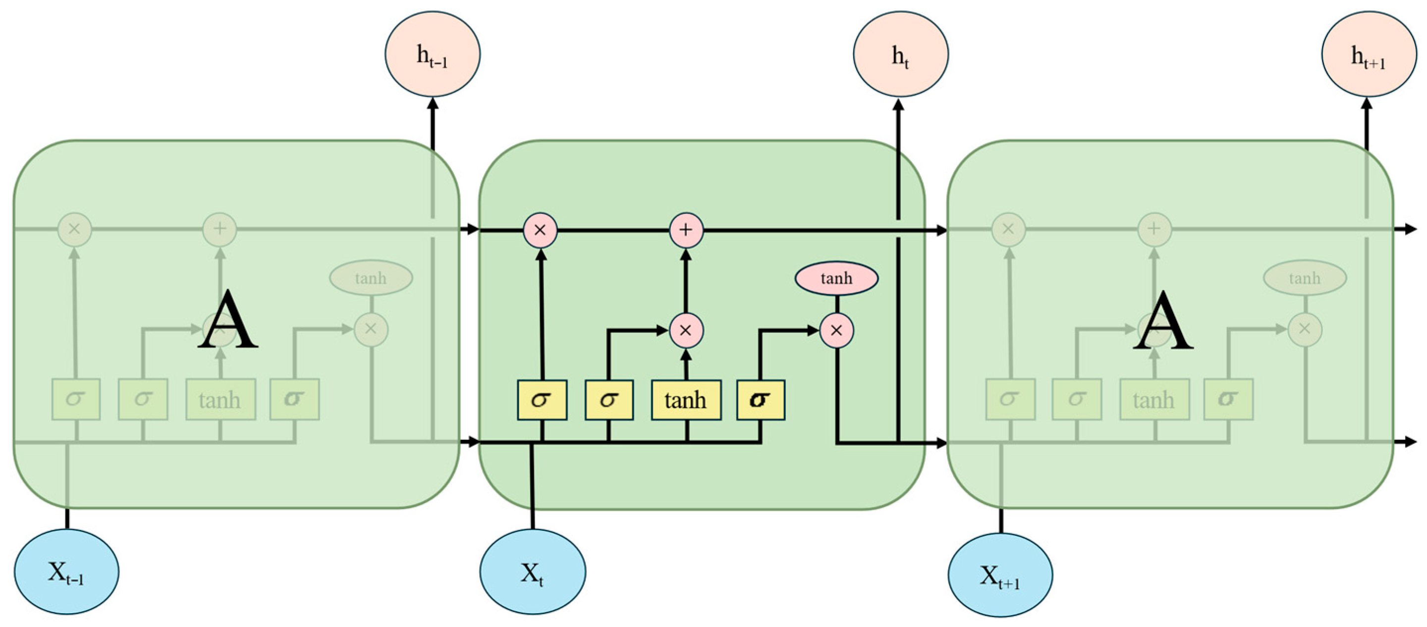
The structure of LSTM is shown in Figure 4. Its primary function is to predict future values by learning from past data [27]. The state of each neuron at every time step is controlled by three gates (input gate, forget gate, and output gate) and the update structure of the state memory unit [28], as described in Equations (1) and (2).

$$\left\{\begin{array}{l}{i}_t=\sigma \left(W_i\cdot [h_{t-1},x_t]+b_i\right)\hfill \\ f_t=\sigma \left(W_f\cdot [h_{t-1},x_t]+b_f\right)\hfill \\ o_t=\sigma \left(W_o\cdot [h_{t-1},x_t]+b_o\right)\hfill \end{array}\right.$$

(1)

$$\left\{\begin{array}{l}{\tilde{C}}_t=\tanh \left(W_c\cdot [h_{t-1},x_t]+b_c\right)\hfill \\ C_t=f_t\ast C_{t-1}+i_t\ast {\tilde{C}}_t\hfill \end{array}\right.$$

(2)

$$h_t=\tanh (C_t)\ast O_t$$

(3)

where $\sigma$ represents the sigmoid function, $W_k$, $b_k$($k=c,f,i,o$) denote the bias and weight matrix terms for the forget gate and input gate, respectively, $h_{t-1}$ is the hidden state output at the time step, $o_t$ and $i_t$ are the activation values for the output gate and input gate, and $C_t$ is the candidate value vector.

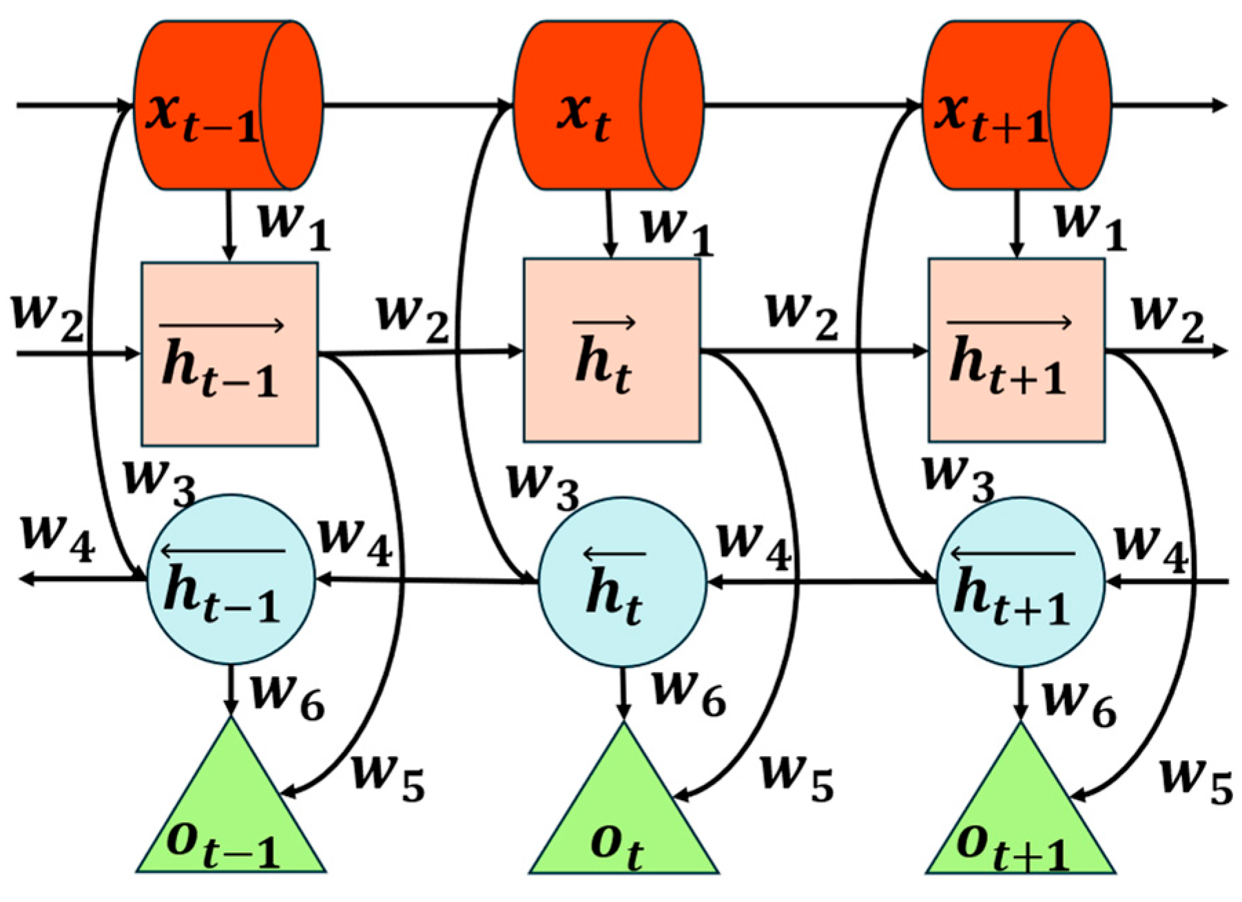
Currently, many time series forecasting models not only consider the impact of historical data on target parameters but also account for the influence of future data changes on these parameters. LSTM exhibits limitations in handling such data variations. Based on this, ref. [29] proposed the BiLSTM model, which considers both historical data and the effects of past data. The BiLSTM structure is shown as Figure 5. The output calculation formula for BiLSTM is presented in Equation (4).

$${\overleftrightarrow{h}}_i=\delta ({\overrightarrow{h}}_i,{\overleftarrow{h}}_i)$$

(4)

where $\delta$ is the function connecting forward and backward inputs, ${\overrightarrow{h}}_i$ denotes the influence of historical project data on fracturing pressure, and ${\overleftarrow{h}}_i$ denotes the influence of future project parameters on fracturing pressure.

2.3. Attention Model

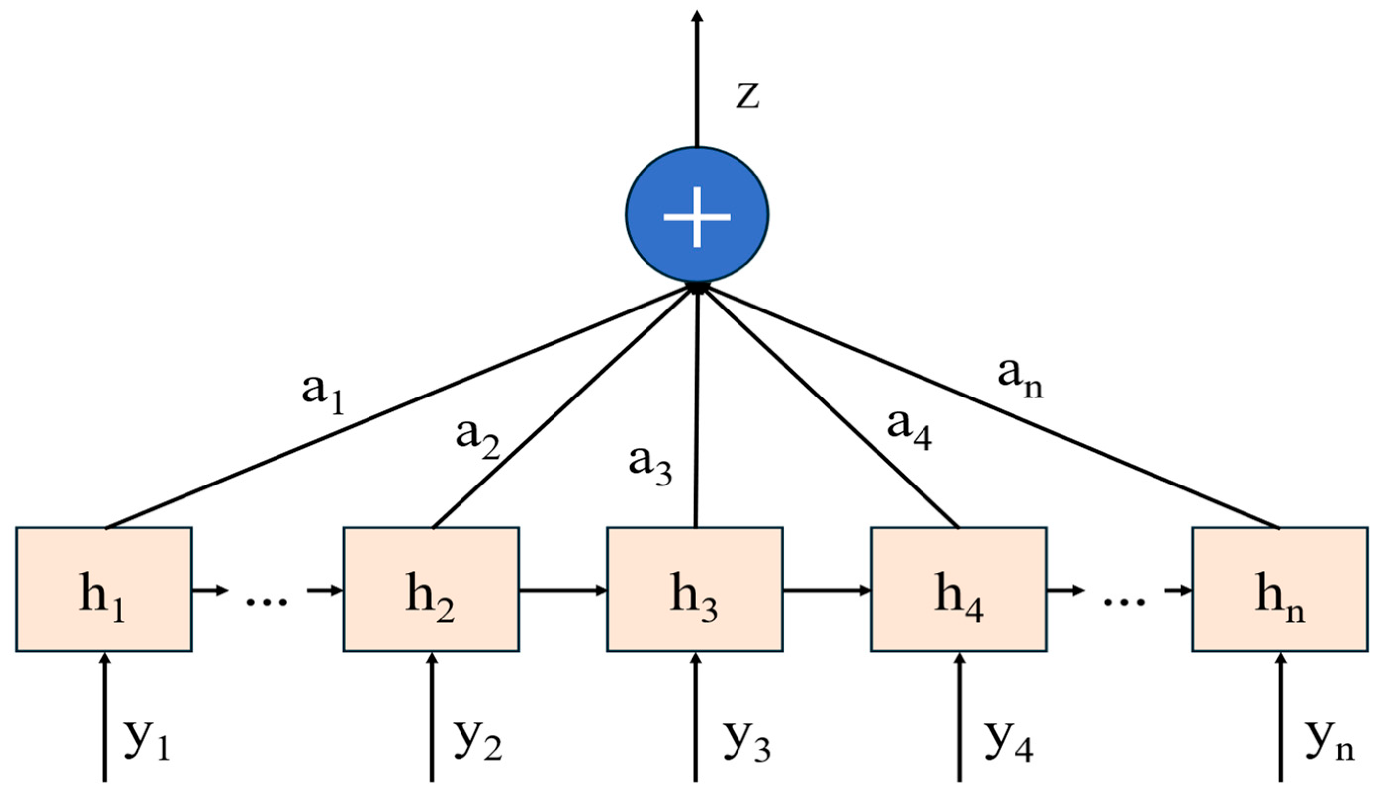
The output of fracturing pressure during the fracturing process is influenced by multiple factors. The temporal variations of each factor interact in complex ways to affect pressure changes. Although BiLSTM is commonly used for time series forecasting, it exhibits limitations in capturing long-term dependencies and dynamic relationships within fracturing engineering data. Therefore, an adaptive approach is required to model these dependencies at a higher level. This study introduces the widely adopted Attention Mechanism, which has demonstrated strong performance across domains, including image classification, object detection, semantic segmentation, video understanding, and image generation [30,31,32]. Attention facilitates representation generation by aggregating information from all time steps within the fracturing operation time series, weighted by varying attention coefficients.

First, compute the input sequences Q, K, and V using the equations shown in Equations (5)–(7).

$$Q=X{W}_Q$$

(5)

$$K=X{W}_K$$

(6)

$$V=X{W}_V$$

(7)

where $W_Q$, $W_K$, and $W_V$ denote the weight matrices used to optimize the fracturing operation parameters. Subsequently, the model normalizes using Q, K, and V, then applies these attention weights A to the value matrix Z to obtain the weighted representation Z, as detailed in Equations (8) and (9).

$$\mathrm{Attention}(Q,K,V)=\mathrm{softmax}\left({\displaystyle \frac{Q{K}^T}{\sqrt{d_k}}}\right)V$$

(8)

$$Z=AV$$

(9)

where $d_k$ represents the dimension of the key vector; Softmax serves as the activation function for multi-class classification; ${\displaystyle \frac{1}{\sqrt{d_k}}}$ is the scaling factor applied to prevent excessively large dot products. This weighted representation effectively integrates information from the entire set of fracturing operation parameters, thereby capturing the intricate variations in fracturing pressure.

The Attention structure, as shown in Figure 6, incorporates an attention mechanism. This enables the model to analyze the relative weights of different features across various time steps, assigning weights to relevant information and allocating higher weights to stronger features to enhance model performance.

3. Feature Analysis and Experimental Design

3.1. Feature Analysis

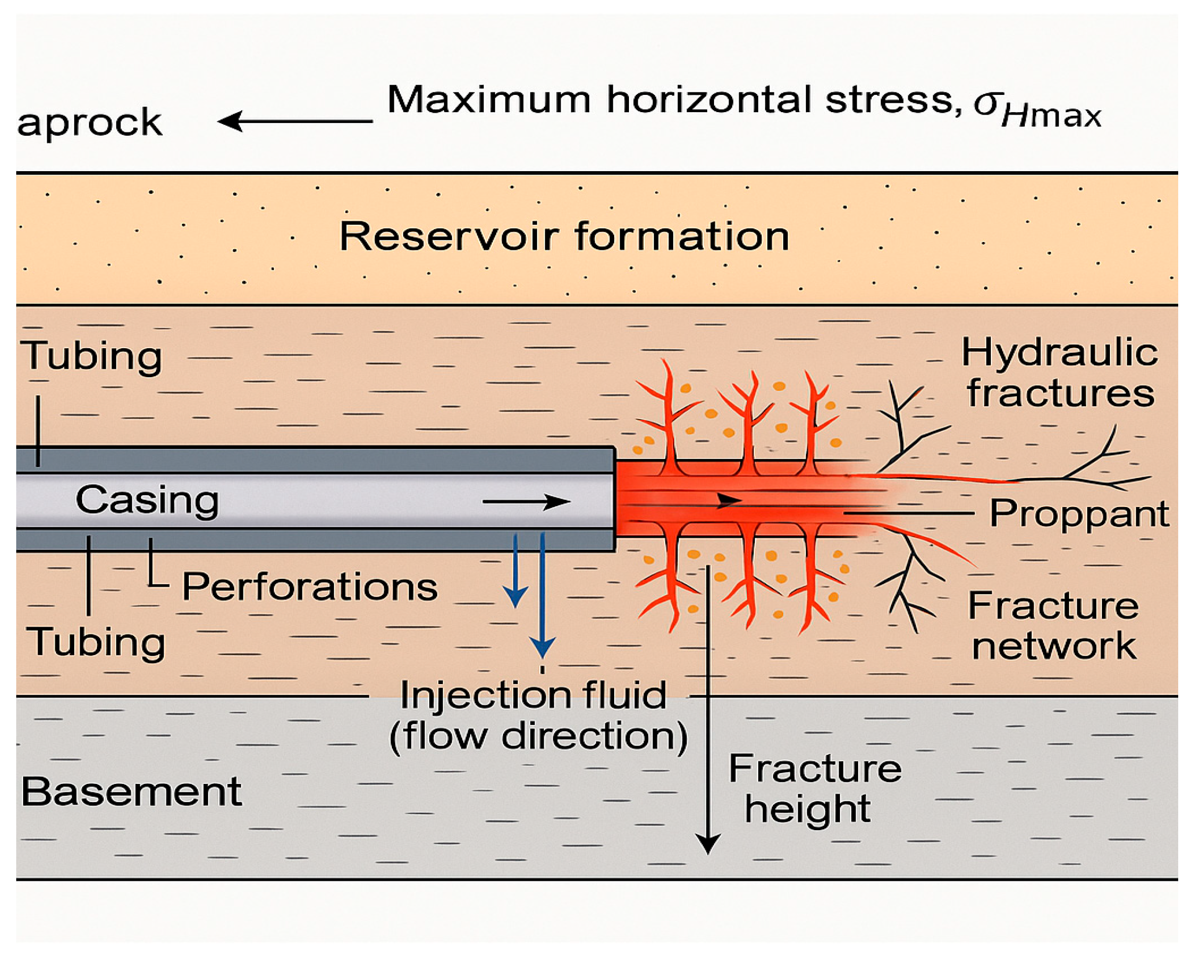
The dataset in this paper originates from the X shale gas block in China’s Sichuan Basin. This resource-rich block has produced a cumulative total of 95 billion cubic meters of natural gas as of September 2025, with proven geological reserves exceeding 1 trillion cubic meters. The study compiled historical hydraulic fracturing operation data for this block, with operational conditions shown in Figure 7.

Based on this, the paper utilizes natural language processing (NLP) technology to extract fracturing operation parameter design documents, obtaining the required detailed data as shown in

Table 1. Fracturing operation parameter data.

Parameter Name	Unit	Min	25%	50%	75%	Max	Mean
Fracturing pressure	MPa	0	75.1	92.22	98.21	115.6	84.21
Pump rate (PR)	m3/min	0	2.03	19.95	20.02	20.47	13.1
Proppant volume fraction (PVF)	%	0	0	0	9	15.1	3.96
Fluid viscosity (FV)	CP	0	20	20	30	41	21.62
Total fluid volume (TFV)	m3	0	255.9	1088.7	1901	2436.3	1100.75
Total proppant volume (TPV)		0	0.7	56.5	107.4	150.4	57.97
Young’s modulus (YM)	GPa	47.47	49.33	58.13	61.53	67.68	51.41
Poisson’s ratio (PRO)		0.27	0.29	0.30	0.31	0.32	0.29
Minimum horizontal stress (MHS)	MPa	85.97	86.38	88.68	90.83	95.84	86.91
Breakdown pressure (BP)	MPa	102.48	103.53	105.96	107.74	113.82	103.84
Brittleness index (BI)		61.78	64.42	68.45	72.97	73.98	66.66

.

As shown in Table 1, these data can be summarized as fracturing engineering parameters, primarily divided into two categories: controllable dynamic parameters such as pump rate, proppant volume fraction, and fluid viscosity; and uncontrollable static data such as Young’s modulus, Poisson’s ratio, and minimum horizontal stress.

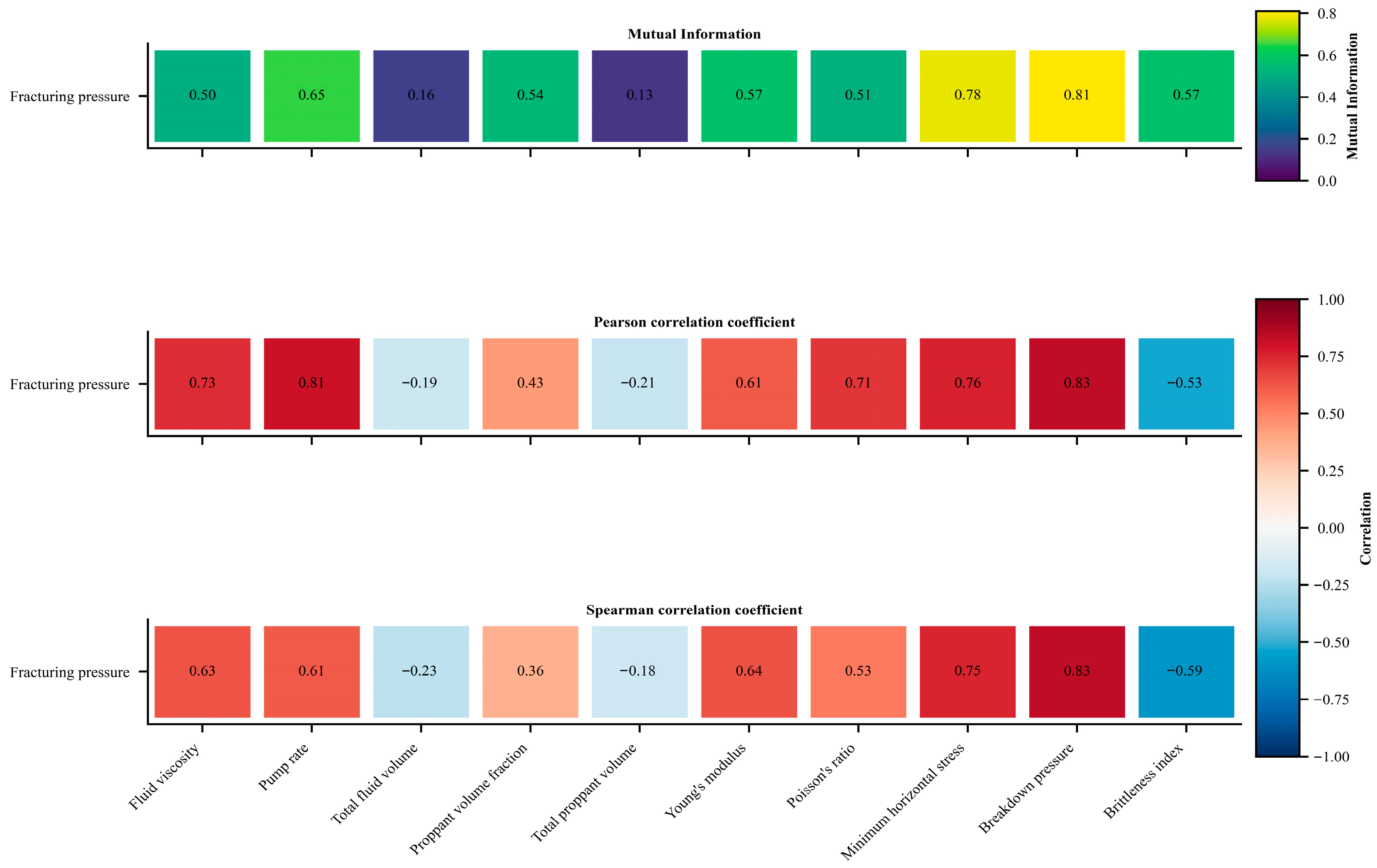
The correlation between target parameters and input parameters is one of the key factors affecting model performance [33,34]. Pearson’s correlation coefficient and Spearman’s analysis are suitable for describing linear relationships between two continuous variables [35,36], making them applicable for selecting data features of fracturing parameters in this study. The Pearson calculation formula is shown in Equation (10), while the Spearman formula is shown in Equation (11).

$$r={\displaystyle \frac{{\displaystyle \sum _{i=1}^n(x_i-\overline{x})}(y_i-\overline{y})}{\sqrt{{\displaystyle \sum _{i=1}^n{(x_i-\overline{x})}^2}}\sqrt{{\displaystyle \sum _{i=1}^n{(y_i-\overline{y})}^2}}}}$$

(10)

where $r$ is the Pearson correlation coefficient, with a value range of [−1, 1]; $n$ is the sample size; $x_i$ and $y_i$ are the i-th observed values of the two variables, respectively; $\overline{x}$ and $\overline{y}$ are the sample means of the two variables, respectively.

$${\rho }_s=1-{\displaystyle \frac{6{\displaystyle \sum d_i^2}}{n(n^2-1)}}$$

(11)

$$d_i=\mathrm{rank}(x_i)-\mathrm{rank}(y_i)$$

(12)

where ${\rho }_s$ denotes the Spearman coefficient, which ranges from −1 to 1. $d_i$ represents the rank difference between the fracturing pressure and target parameters. $\mathrm{rank}(x_i)$ indicates the rank of sample $x_i$ in X, while $\mathrm{rank}(y_i)$ denotes the rank of sample $y_i$ in Y. ${\displaystyle \sum d_i^2}$ signifies the sum of squared rank differences across all samples; a smaller value indicates greater consistency in the order of the two variables and stronger correlation. $n(n^2-1)$ represents the normalization factor.

Correlation analysis can only reveal linear relationships between fracturing pressure and other parameters. However, variations in fracturing pressure are not solely governed by linear relationships; they also involve nonlinear relationships, which are equally significant. Mutual information analysis, a commonly used method for examining nonlinear relationships [37], employs the calculation formula shown in Equation (13).

$$I(X;Y)={\displaystyle \sum _{i,j}p}(x_i,y_j)\log {\displaystyle \frac{p(x_i,y_j)}{p(x_i)p(y_j)}}$$

(13)

where $I(X;Y)$ denotes the nonlinear relationship between the random engineering parameter X and the objective parameter fracturing pressure, and $p(x_i,y_j)$ represents the joint probability distribution, i.e., the probability that $X=x_i$ and $Y=y_i$ occur simultaneously. is the ratio of the probability that $X$ and $Y$ occur together to the probability that they occur independently.

Based on the correlation analysis results in Figure 8, it can be observed that among the input parameters, FV, PR, YM, PRO, MHS, BP, and BI exhibit strong correlations with fracturing pressure. Meanwhile, PVF exhibits moderate correlations in both Pearson and Spearman analyses, but a stronger correlation in mutual information analysis. Some of the literature studies also treat PVF as an input parameter [38] since it can cause sand blockage in fractures, leading to fracturing pressure surges. Therefore, PVF is also included as an input feature. TPV and TFV exhibit weak correlations with fracturing pressure across all three correlation analyses and are thus excluded as input parameters.

This paper first performs preliminary screening based on Pearson, Spearman, and mutual information metrics to eliminate features exhibiting high multicollinearity and weak correlations. To further validate the actual contribution of each input feature to predictive performance, feature ablation experiments are conducted on the model using evaluation metrics. Common evaluation metrics such as MAE, R², and RMSE effectively reflect variations in pressure predictions [39]. Therefore, these three metrics are adopted as evaluation indicators for fracturing pressure prediction, with their calculation formulas as shown in the Equations (14)–(16).

$$MAE={\displaystyle \frac{1}{N}}{\displaystyle \sum _{i=1}^n|}{y}_i-{\widehat{y}}_i|$$

(14)

$$R^2=1-{\displaystyle \frac{{\displaystyle \sum _{i=1}^n{(y_i-{\widehat{y}}_i)}^2}}{{\displaystyle \sum _{i=1}^n{(y_i-\overline{y})}^2}}}$$

(15)

$$RMSE=\sqrt{{\displaystyle \frac{1}{N}}{\displaystyle \sum _{i=1}^{\mathrm{n}}{(y_i-{\widehat{y}}_i)}^2}}$$

(16)

where $y_i$ represents the actual fracturing pressure value, ${\widehat{y}}_i$ represents the model-predicted fracturing pressure value, and $N$ denotes the size of the dataset. The smaller the values of MAE and RMSE, the higher the prediction accuracy of the model; these values cannot be negative. The closer R² is to 1, the higher the variance in the data explained by the model and the better the prediction performance. The data range is [0, 1].

This study conducted ablation experiments by sequentially removing individual features while retaining the full-feature model as a baseline, then retraining the model to compare changes in MAE, RMSE, and R² on the test set. As shown in

Table 2. Ablation experiment results.

Unentered Feature	MAE	RMSE	R2
PR	1.8853	1.3279	0.8921
PVF	1.5632	1.7842	0.8525
FV	1.8643	1.4521	0.8352
TFV	0.5703	0.8423	0.9525
TPV	0.6832	0.9212	0.9429
YM	0.7409	1.1242	0.8851
PRO	0.8615	1.2821	0.8955
MHS	0.8489	1.3956	0.8845
BP	1.8588	1.4757	0.8709
BI	1.3109	1.6715	0.8931

, omitting PVF and FV significantly reduces model accuracy, whereas removing TFV and TPV has a minor impact on performance. The model evaluating all input features yielded overall performance metrics of MAE = 0.5423 MPa, RMSE = 0.8159 MPa, and R² = 0.9576. After removing TFV, the model’s MAE increased by 0.028 MPa, the RMSE rose by 0.0246 MPa, and the R² decreased by 0.0051. This suggests that removing TFV has a negligible impact on the model, resulting in minimal changes in evaluation metrics. After removing TPV, the model’s MAE increased by 0.1409 MPa, RMSE rose by 0.1053 MPa, and R² decreased by 0.0147. Therefore, TFV and TPV exhibit low predictive contribution and are redundant features that can be removed from the model to simplify its structure and enhance computational efficiency. This indicates that core construction parameters contribute more substantially to fracture pressure prediction, while auxiliary variables primarily serve a corrective role. TFV and TPV are redundant parameters. Therefore, the input features for this study comprise eight variables: FV, PR, PVF, YM, PRO, MHS, BP, and BI. The feature selection results are shown in

Table 3. Feature selection results.

Parameter Name	Pearson Correlation	Spearman’s Correlation	MC	Melting Experiment	Whether to Choose
Fluid viscosity	√	√	√	√	Yes
Pump rate	√	√	√	√	Yes
Total fluid volume	×	×	×	×	No
Proppant volume fraction	×	×	√	√	Yes
Total proppant volume	×	×	×	×	No
Young’s modulus	√	√	√	√	Yes
Poisson’s ratio	√	√	√	√	Yes
Minimum horizontal stress	√	√	√	√	Yes
Breakdown pressure	√	√	√	√	Yes
Brittleness index	√	√	√	√	Yes

.

Normalization effectively enhances prediction accuracy, improves model stability, and ensures regularization effects [40]. Due to differing units among feature parameters in the dataset, hidden influence relationships may be overlooked during model analysis. To accelerate model convergence and enhance stability and accuracy [41], considering that the data in this paper is distributed within an interval range, we employ maximum–minimum normalization to map fracturing operation data to the [0, 1] interval. The calculation formula is shown in the Equation (17).

$$X_i={\displaystyle \frac{x_i-\min (x_i)}{\max (x_i)-\min (x_i)}}$$

(17)

where $x_i$ represents the raw feature data, and $X_i$ represents the normalized feature values.

To evaluate the generalization capability of the proposed prediction model, it was compared with three benchmark models: LSTM, BiLSTM, and TCN-BiLSTM. To ensure the accuracy of the model comparison, a batch size of 256 for model input, the random seed count is 42, and the Adam optimizer is used. Model hyperparameters are one factor influencing model robustness [42]. Therefore, the commonly used parameter optimizer hyperopt was employed for parameter tuning [43]. For detailed information on the specific parameters of the prediction models used in the experiments, please refer to

Table 4. Model parameter settings.

Model	Parameter	Value
TCN	Layers	2
	Filters	128/256
	Kernel size	3/5
	Dropout	0.3
LSTM/BiLSTM	Layers	2
	Units	256/512
	Dropout	0.3
Attention	Heads	4
	Key	8
	Hidden	64
	Dropout	0.3
Learning rate		0.001
Activation function		ReLU

.

All experiments were conducted using a PyTorch 2.7.1 + CUDA 12.8 environment. The platform hardware specifications are as follows: Operating System: Windows 10, Processor: Intel Core i5-12490F, clocked at 4.6 GHz, Graphics Card: NVIDIA GeForce RTX 5070 Ti (16GB), CPU: 64 GB.

3.2. Experimental Design

To evaluate the predictive performance of the proposed model in this study, we designed a series of experiments to validate the algorithm’s effectiveness and assess the impact of different prediction models on the results. We compared the proposed model against LSTM, BiLSTM, and TCN-BiLSTM as benchmark models. This evaluation enabled us to verify their influence on the outcomes.

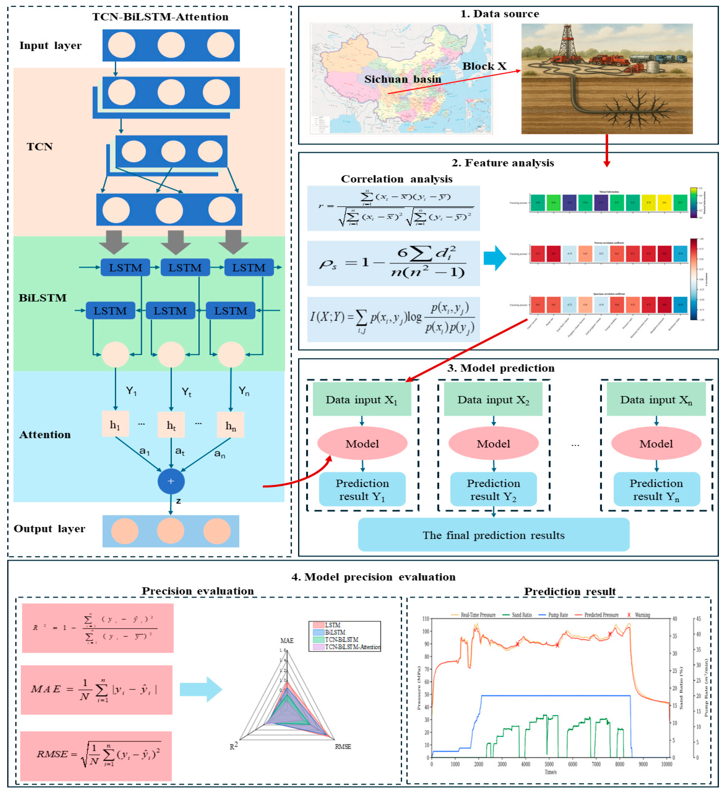
The experimental design is illustrated in Figure 9, outlining four key stages of the process. The first stage involves data sourcing, where historical fracturing operation data was obtained from Block X in the Sichuan Basin. This dataset was utilized for comparative fracturing pressure prediction experiments. The second stage involves feature analysis, where linear and nonlinear correlation analyses are performed on data characteristics to eliminate irrelevant features and prevent redundant data from impacting the model. The third stage involves implementing the prediction model. A TCN-BiLSTM-Attention-based prediction model, a multi-input single-output model, was employed. Through model training, future fracturing pressure data were obtained. Finally, model performance evaluation was conducted. This study employed three proposed evaluation metrics to compare model predictions with actual observations, verifying the model’s validity. Additionally, percentage metrics were used to quantitatively analyze the contribution of different model components to the overall improvement when comparing the proposed model with reference models.

4. Application Cases

4.1. Comparison of Pressure Prediction Models

To validate the proposed prediction model, this study utilized 10 completed fracturing stages from adjacent well sections within Block X or from strata with similar conditions as the validation set. Considering the delayed transmission characteristics of field data sensors, the dataset and test set were divided at a 4:1 ratio to assess the model’s performance. Two fracturing stages from Block X were designated as the target prediction stages, with the two validation sets named Dataset 1 and Dataset 2.

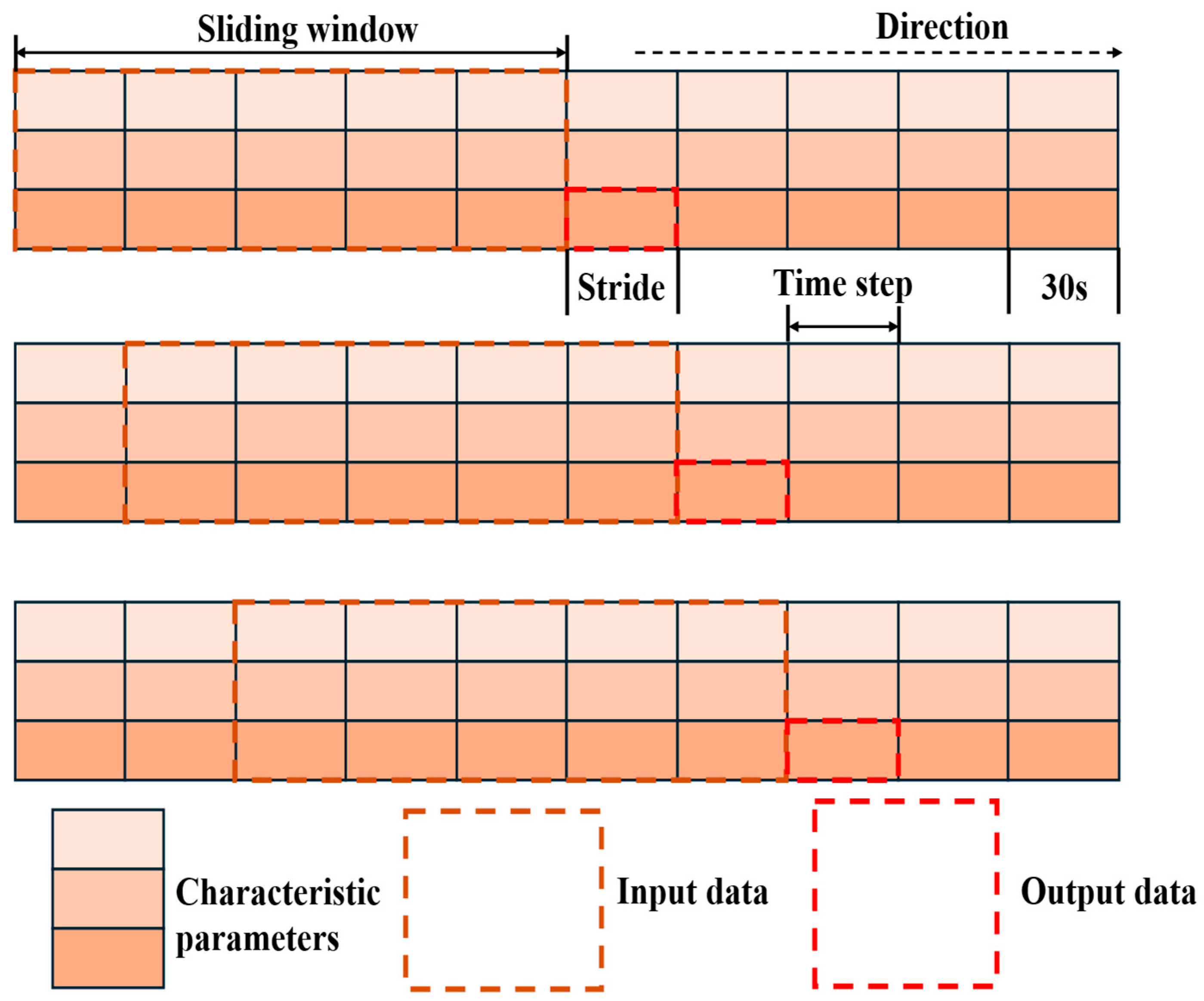
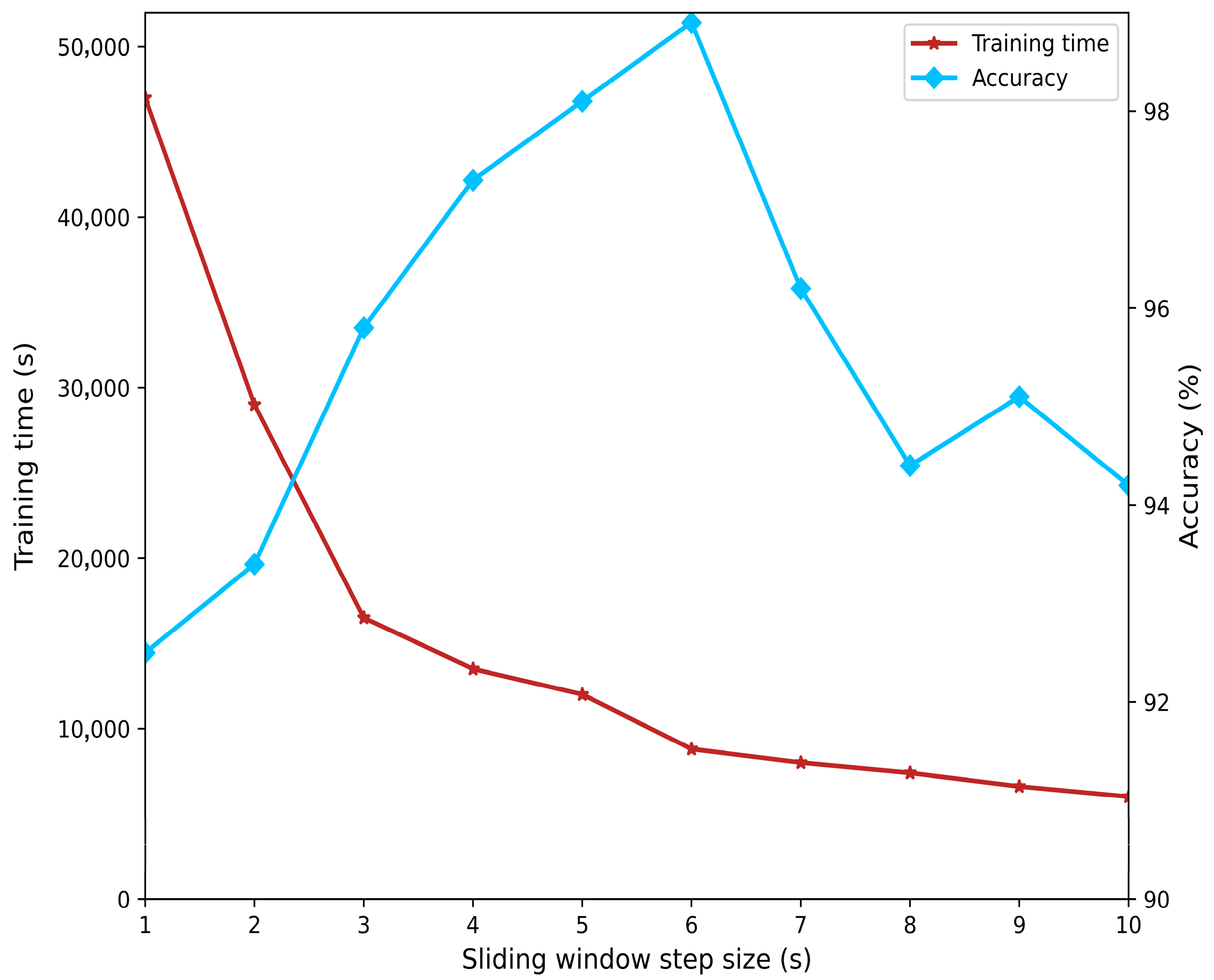
The sliding window is a key component in time series model forecasting, effectively converting historical data into a format suitable for time series analysis, as illustrated in Figure 10. As shown in Figure 11, a sliding window stride of n = 6 enables the model to avoid introducing excessive noise or overfitting while achieving optimal training time and model performance.

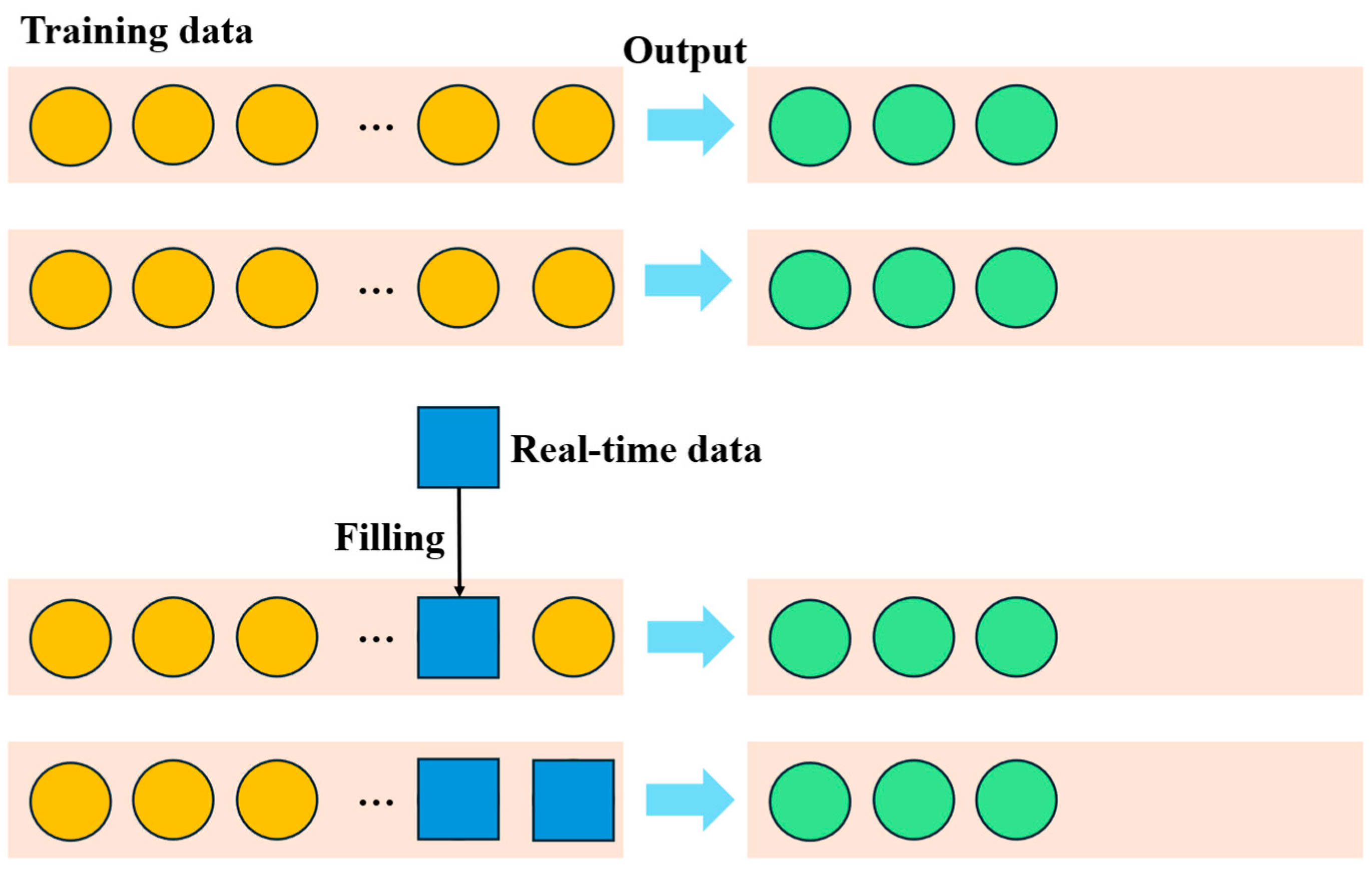
Currently, data transmission in Block X exhibits latency, which prevents the delivery of real-time data for real-time models. Therefore, this study accounts for the data transmission delay of 180 s in this oilfield. Based on a sliding window time step of 6 s, the window size and prediction step are set as shown in

Table 5. Sliding window setting.

Parameter	Value
Window length (s)	180
Prediction step size (s)	30

. Data from the 4th minute serves as the output. Parameter data from the 2nd to 4th minutes form the input for the second sample. The fracturing pressure variation in the 5th minute constitutes the output for the third sample. Subsequent processes repeat this procedure. However, to enhance the model’s predictive performance, real-time data is integrated during the prediction phase. To mitigate error propagation in the prediction process, predicted values from the training samples are dynamically replaced with actual data in real time, creating a recursive process. This process is illustrated in Figure 12.

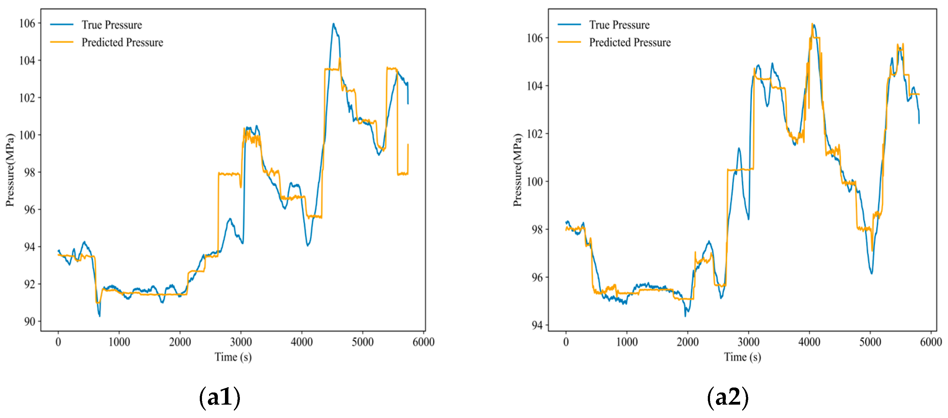
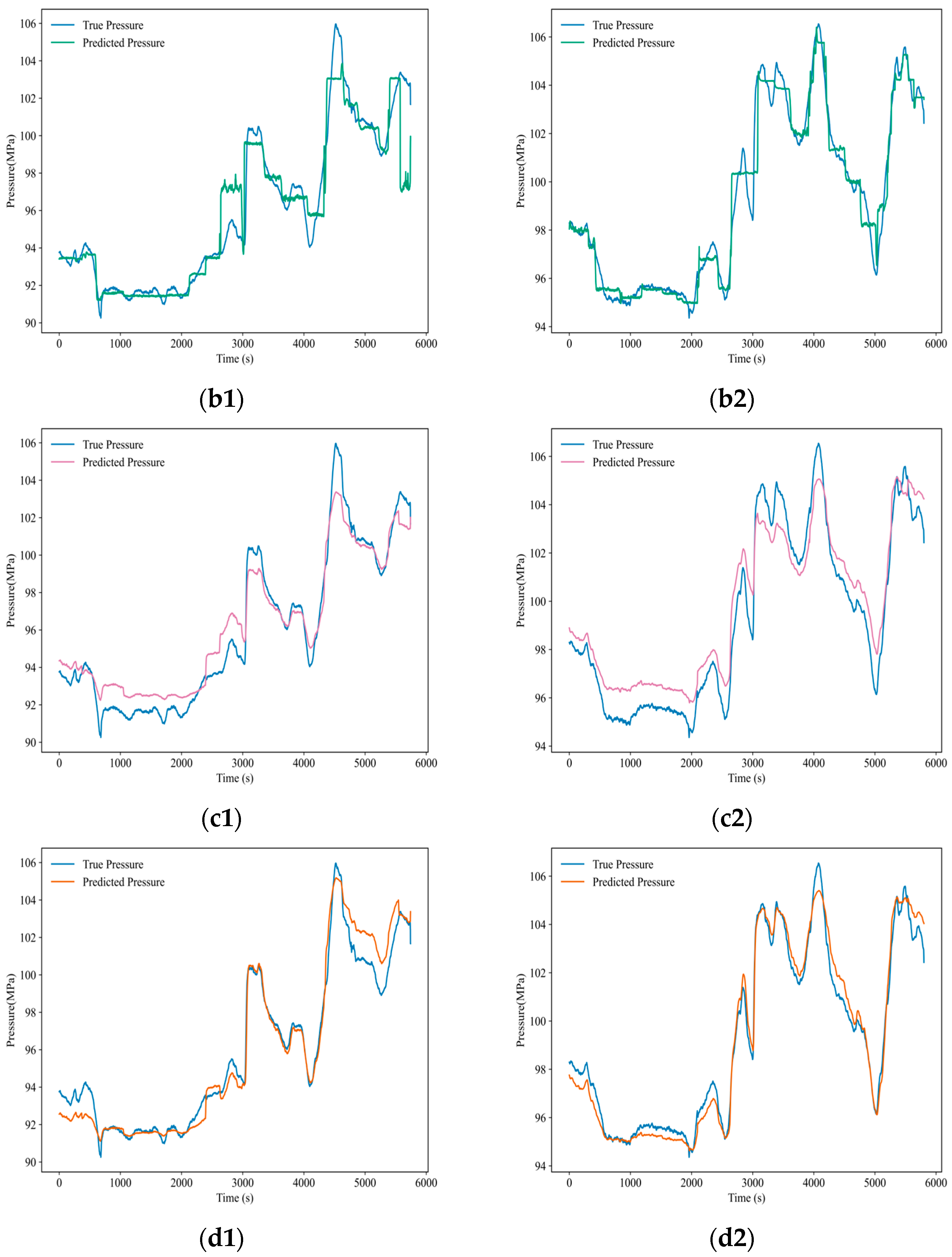
Four models were trained for prediction, yielding the results shown in Figure 13. As depicted in Figure 13, the trends of fracturing pressure predictions from all four models generally align with the actual fracturing pressure trends. In terms of prediction accuracy, the fracturing pressure curve predicted by the TCN-BiLSTM-Attention model most closely matches the actual fracturing pressure curve.

As shown in Figure 13a1,a2,b1,b2, both LSTM and BiLSTM models demonstrate strong performance in predicting fracturing pressure. However, when dealing with small-amplitude pressure fluctuations, both models exhibit trapezoidal patterns, resulting in prediction outcomes that fail to meet expected requirements. Figure 13c1,c2 reveals that incorporating TCN effectively captures local numerical fluctuations, successfully resolving the trapezoidal prediction issue and thereby enhancing the model’s predictive accuracy.

As observed in Figure 13c1,c2, the TCN-BiLSTM demonstrates promising properties during fracture pressure prediction. However, it fails to capture nonlinear relationships among data points during certain local fluctuations. Comparing Figure 13d1,d2 reveals that incorporating Attention effectively captures feature variation relationships. The proposed TCN-BiLSTM-Attention achieves the best prediction performance compared to LSTM, BiLSTM, and TCN-BiLSTM models, showing substantial agreement with the true curve results.

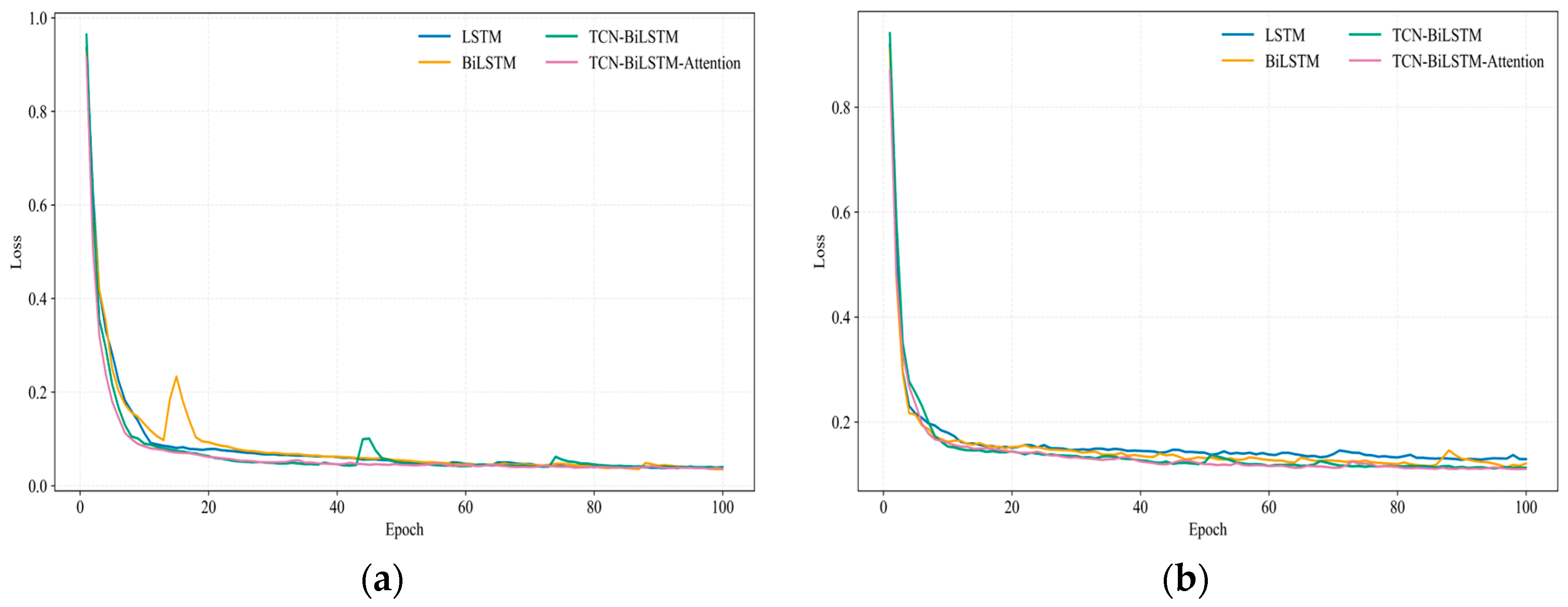
The convergence process of various models’ loss functions on the training dataset is shown in Figure 14. It can be observed that during the first 100 training iterations, the TCN-BiLSTM-Attention model converges faster than the other models as the iteration count increases. After parameter stabilization, it achieves a lower loss value. This indicates that compared to LSTM, BiLSTM, and TCN-BiLSTM, the TCN-BiLSTM-Attention model exhibits the fastest convergence speed during training.

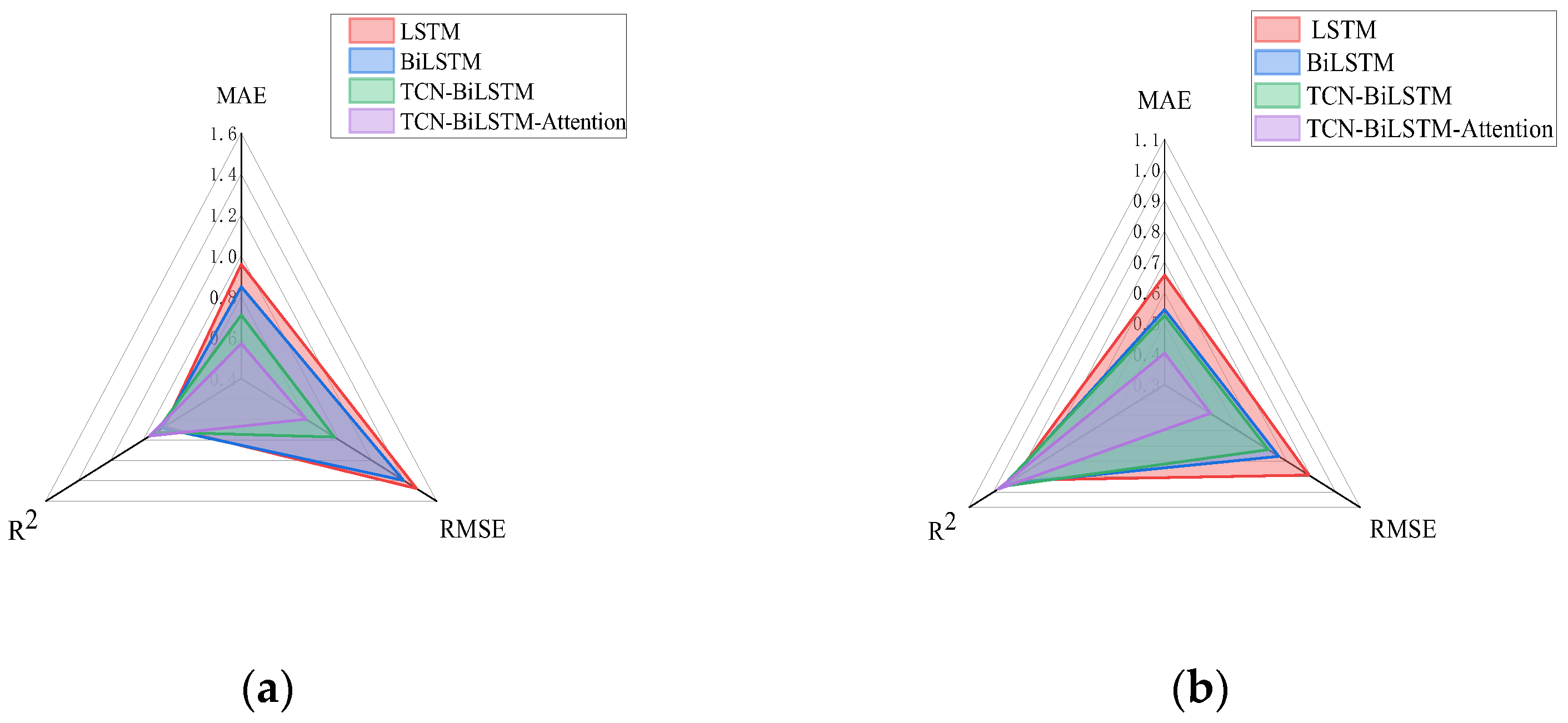
As shown in

Table 6. Evaluation metric results for Datasets 1 and 2.

Model	Dataset 1			Dataset 2
	MAE	RMSE	R2	MAE	RMSE	R2
LSTM	0.9588	1.4757	0.8709	0.6573	0.8895	0.9232
BiLSTM	0.8489	1.3956	0.8845	0.5447	0.7671	0.9454
TCN-BiLSTM	0.7109	0.9715	0.9231	0.5258	0.7238	0.9631
TCN-BiLSTM-Attention	0.5709	0.7978	0.9621	0.4027	0.4867	0.9816

and Figure 15, compared to LSTM, BiLSTM achieved a 13.76% reduction in average MAE and an 8.56% reduction in RMSE, while improving by 1.98%. This demonstrates that the bidirectional LSTM achieves significant improvements over the unidirectional LSTM. Compared to BiLSTM, TCN-BiLSTM achieved an 11.27% reduction in MAE and a 21.61% reduction in RMSE, while improving by 3.08%. This demonstrates that BiLSTM’s performance significantly improved after capturing feature variations through TCN. Compared to TCN-BiLSTM, TCN-BiLSTM-Attention reduced MAE by 21.27% and RMSE by 24.24%, while improving accuracy by 3.04%. This demonstrates that incorporating Attention positively impacts TCN-BiLSTM, enhancing the overall model’s robustness. Therefore, experiments demonstrate that the proposed TCN-BiLSTM-Attention achieves the highest fracturing pressure prediction accuracy and fastest computational efficiency among the four models.

4.2. On-Site Application

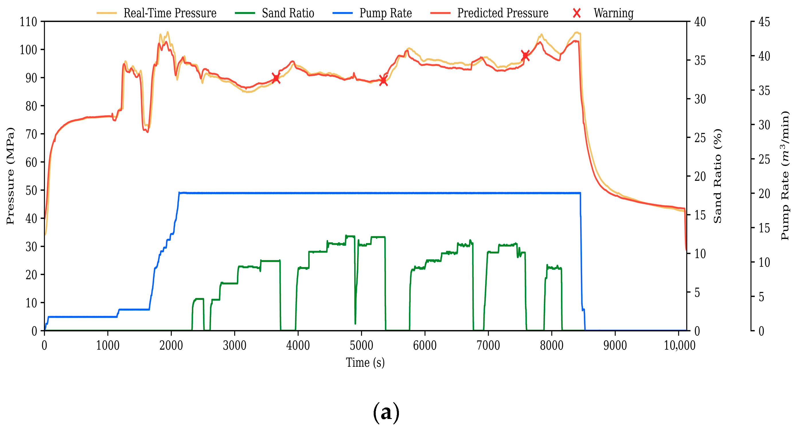
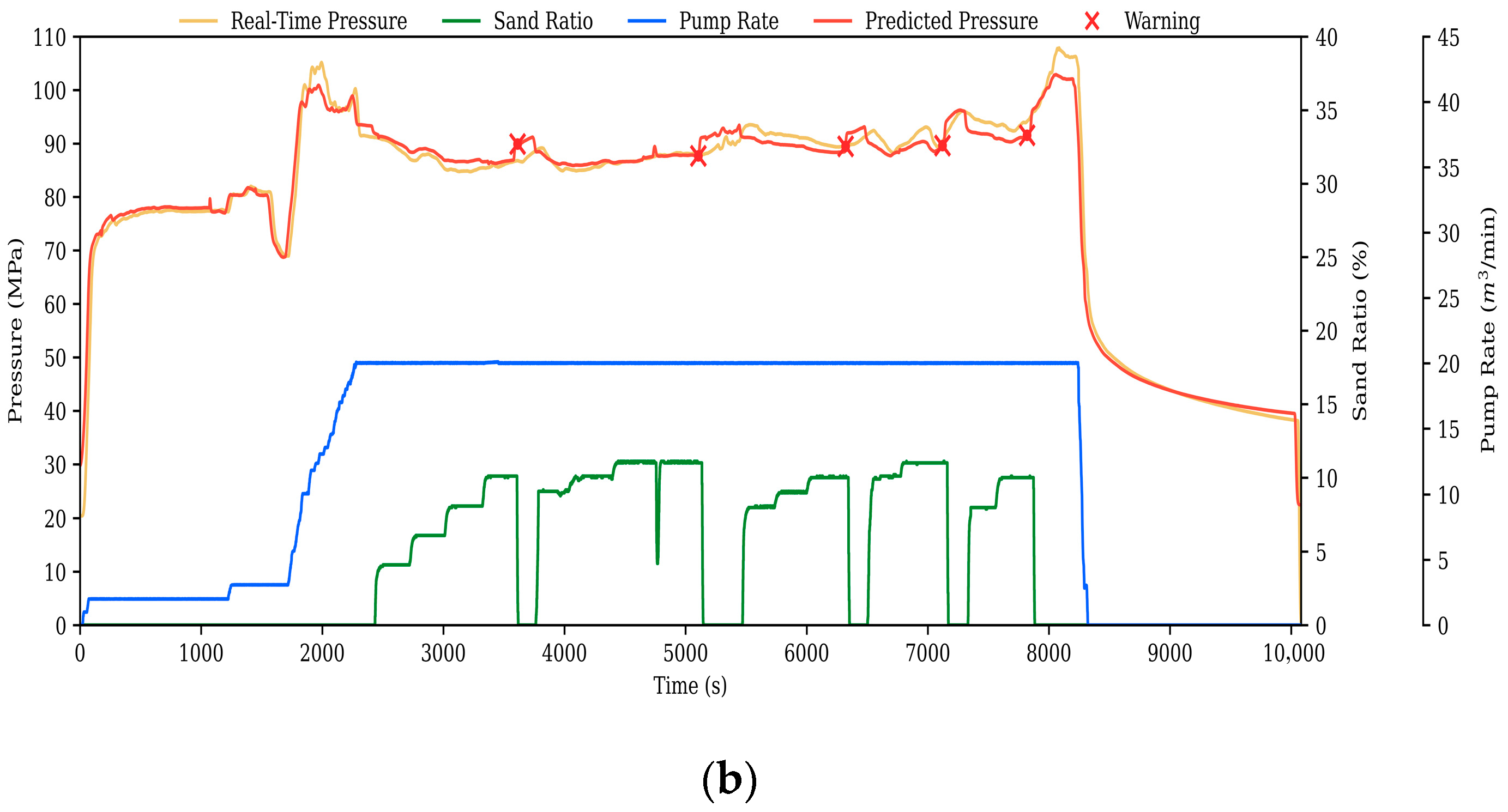
Relying solely on model comparisons is insufficient to demonstrate the proposed model’s applicability in actual engineering projects. To evaluate its field implementability and diagnostic value, this study conducted field application verification during fracturing operations in Block X. Conventional operations in this block rely on abnormal fluctuations in fracturing pressure curves for risk assessment, employing the slope reversal method [44] as an empirical criterion for determining the likelihood of sand screenout occurrence. Without altering the existing field workflow, this study overlaid the developed fracture pressure prediction model against measured pressure curves and employed the slope reversal method for sand screenout early warning. Field validation was conducted on two representative operational sections (Validation set A and Validation set B), yielding Figure 16.

The proposed fracturing pressure prediction model effectively replicates the temporal evolution of pressure in two field validation datasets, exhibiting high consistency with measured curves in both trend and fluctuation amplitude (see Figure 16). Error evaluation metrics listed in

Table 7. Test set evaluation metrics.

Section Name	MAE	RMSE	R2
Validation section A	0.9722	1.0126	0.9877
Validation section B	1.3135	1.2037	0.9868

(e.g., MAE, RMSE, and R²) remain at low levels, indicating minimal deviation between predicted and measured curves and high fitting accuracy. Furthermore, comparing the model’s warning points (identified using the “prediction result + slope reversal method”) with the manual sand-stopping times in

Table 8. Comparison of models and manual alerts.

Well Section Name	Model Warning Point	Manual Sand Control Point
Validation section A	3652 s	3727 s
Validation section A	5347 s	5382 s
Validation section A	7582 s	7604 s
Validation section B	3612 s	3619 s
Validation section B	5105 s	5147 s
Validation section B	6321 s	6354 s
Validation section B	7121 s	7170 s
Validation section B	7819 s	7884 s

, the model achieved early warnings for all eight pressure surge events identified in the two validation sets, with an average warning time of 41 s (minimum: 7 s, maximum: 75 s). These results demonstrate the model’s robust real-time predictive capability and engineering application potential in actual construction environments.

5. Conclusions

This paper proposes a fracturing pressure prediction model based on multi-source information fusion, offering a novel approach for fracturing pressure forecasting. The new method employs data from adjacent wells or wells with identical geological conditions for training, enabling transfer to new blocks through a transfer learning strategy. Key conclusions are as follows.

(1) Considering the characteristics of data collected during hydraulic fracturing operations, Pearson correlation analysis, Spearman correlation analysis, and mutual information methods were employed to screen input features. Following analysis, fluid viscosity, pump rate, proppant volume fraction, Young’s modulus, Poisson’s ratio, minimum horizontal stress, breakdown pressure, and brittleness index were selected as input parameters to reduce the impact of redundant data on model prediction.

(2) Introducing TCN as a feature extractor addresses the limitation of BiLSTM models in capturing the impact of local data feature fluctuations on model performance. Experimental results demonstrate that the proposed TCN-BiLSTM-Attention architecture exhibits significant advantages in prediction accuracy and reliability compared to standalone DL models.

(3) The “prediction–criterion combined identification” framework, which integrates model outputs with the slope reversal method, enables proactive identification of sand plugging risks. In the eight pressure surge events identified across two validation sets, the combined approach provided an average warning of 41 s compared to manual sand plugging shutdowns, demonstrating clear real-time application value.

In summary, the model demonstrates field applicability and decision-making support value, with the potential to reduce sand-blocking risks and enhance construction safety and efficiency.

References

1. Chen, B.; Barboza, B.R.; Sun, Y.; Bai, J.; Thomas, H.R.; Dutko, M.; Cottrell, M.; Li, C. A review of hydraulic fracturing simulation. Arch. Comput. Methods Eng. 2021, 29, 1–58. [Google Scholar] [CrossRef]
2. Nolte, K.G.; Smith, M.B. Interpretation of fracturing pressures. J. Pet. Technol. 1981, 33, 1767–1775. [Google Scholar] [CrossRef]
3. Nguyen, H.T.; Lee, J.H.; Elraies, K.A. A review of PKN-type modeling of hydraulic fractures. J. Pet. Sci. Eng. 2020, 195, 107607. [Google Scholar] [CrossRef]
4. Gladkov, I.; Linkov, A. Khristianovich-Geertsma-de Klerk problem with stress contrast. arXiv 2017, arXiv:1703.05686. [Google Scholar] [CrossRef]
5. Ferguson, W.; Richards, G.; Bere, A.; Mutlu, U.; Paw, F. Modelling near-wellbore hydraulic fracture branching, complexity and tortuosity: A case study based on a fully coupled geomechanical modelling approach. In Proceedings of the SPE Hydraulic Fracturing Technology Conference and Exhibition, The Woodlands, TX, USA, 23–25 January 2018; p. D021S004R001. [Google Scholar]
6. Jordan, M.I.; Mitchell, T.M. Machine learning: Trends, perspectives, and prospects. Science 2015, 349, 255–260. [Google Scholar] [CrossRef] [PubMed]
7. Qiu, J.; Wu, Q.; Ding, G.; Xu, Y.; Feng, S. A survey of machine learning for big data processing. EURASIP J. Adv. Signal Process. 2016, 2016, 67. [Google Scholar] [CrossRef]
8. LeCun, Y.; Bengio, Y.; Hinton, G. Deep learning. Nature 2015, 521, 436–444. [Google Scholar] [CrossRef]
9. Brenjkar, E.; Delijani, E.B. Engineering. Computational prediction of the drilling rate of penetration (ROP): A comparison of various machine learning approaches and traditional models. J. Pet. Sci. Eng. 2022, 210, 110033. [Google Scholar] [CrossRef]
10. Matinkia, M.; Sheykhinasab, A.; Shojaei, S.; Vojdani Tazeh Kand, A.; Elmi, A.; Bajolvand, M.; Mehrad, M. Engineering. Developing a new model for drilling rate of penetration prediction using convolutional neural network. Arab. J. Sci. Eng. 2022, 47, 11953–11985. [Google Scholar] [CrossRef]
11. Xu, K.; Liu, Z.; Chen, Q.; Zhang, Q.; Ling, X.; Cai, X.; He, Q.; Yang, M. Engineering. Application of machine learning in wellbore stability prediction: A review. Geoenergy Sci. Eng. 2024, 232, 212409. [Google Scholar] [CrossRef]
12. Gao, J.; Chen, F.; Zhang, P.; Wang, Q.; Wu, Y.; Bian, G.; Yang, W. Probabilistic Inversion of Horizontal In Situ Stresses Combining Bayesian Theory and Borehole Failure Data to Quantify the Uncertainty of Wellbore Instability Risk. Rock Mech. Rock Eng. 2025, 1–30. [Google Scholar] [CrossRef]
13. Gao, J.; Yang, W.; Chen, F.; Chang, L.; Lin, H.; Feng, Y.; Bian, G.; Jiang, H. Pore Pressure Prediction Using Machine Learning Methods and Logging Data Considering Gaussian Mixture Clustering Model. Geoenergy Sci. Eng. 2025, 257, 214188. [Google Scholar] [CrossRef]
14. Wang, S.; Qin, C.; Feng, Q.; Javadpour, F.; Rui, Z. A framework for predicting the production performance of unconventional resources using deep learning. Appl. Energy 2021, 295, 117016. [Google Scholar] [CrossRef]
15. Zhou, G.; Guo, Z.; Sun, S.; Jin, Q. A CNN-BiGRU-AM neural network for AI applications in shale oil production prediction. Appl. Energy 2023, 344, 121249. [Google Scholar] [CrossRef]
16. Madasu, S.; Rangarajan, K.P. Deep recurrent neural network DRNN model for real-time multistage pumping data. In Proceedings of the OTC Arctic Technology Conference, Houston, TX, USA, 5–7 May 2018; p. D033S017R005. [Google Scholar]
17. Hu, J.; Khan, F.; Zhang, L.; Tian, S. Data-driven early warning model for screenout scenarios in shale gas fracturing operation. Comput. Chem. Eng. 2020, 143, 107116. [Google Scholar] [CrossRef]
18. Liang, H.; Zou, J.; Khan, M.J.; Jinxuan, H. An sand plug of fracturing intelligent early warning model embedded in remote monitoring system. IEEE Access 2019, 7, 47944–47954. [Google Scholar] [CrossRef]
19. Hou, L.; Zhou, L.; Elsworth, D.; Wang, S.; Wang, W. Prediction of fracturing pressure and parameter evaluations at field practical scales. Rock Mech. Rock Eng. 2024, 57, 2567–2580. [Google Scholar] [CrossRef]
20. Sun, J.J.; Battula, A.; Hruby, B.; Hossaini, P. Application of both physics-based and data-driven techniques for real-time screen-out prediction with high frequency data. In Proceedings of the SPE/AAPG/SEG Unconventional Resources Technology Conference, Houston, TX, USA, 20–22 July 2020; p. D023S027R003. [Google Scholar]
21. Bin, Y.; Mingze, Z.; Siwei, M. Intelligent identification and real-time warning method of diverse complex events in horizontal well fracturing. Pet. Explor. Dev. 2023, 50, 1487–1496. [Google Scholar] [CrossRef]
22. Yuan, Y.; Zhou, K.; Zhou, W.; Wen, X.; Liu, Y. Flow prediction using dynamic mode decomposition with time-delay embedding based on local measurement. Phys. Fluids 2021, 33, 095109. [Google Scholar] [CrossRef]
23. Shah, S.; Wilder, B.; Perrault, A.; Tambe, M. Leaving the nest: Going beyond local loss functions for predict-then-optimize. In Proceedings of the AAAI Conference on Artificial Intelligence, Vancouver, BC, Canada, 20–27 February 2024; pp. 14902–14909. [Google Scholar]
24. Lea, C.; Flynn, M.D.; Vidal, R.; Reiter, A.; Hager, G.D. Temporal convolutional networks for action segmentation and detection. In Proceedings of the IEEE Conference on Computer Vision and Pattern Recognition, Honolulu, HI, USA, 21–26 July 2017; pp. 156–165. [Google Scholar]
25. Fan, J.; Zhang, K.; Huang, Y.; Zhu, Y.; Chen, B. Parallel spatio-temporal attention-based TCN for multivariate time series prediction. Neural Comput. Appl. 2023, 35, 13109–13118. [Google Scholar] [CrossRef]
26. Li, Y.; Song, L.; Zhang, S.; Kraus, L.; Adcox, T.; Willardson, R.; Komandur, A.; Lu, N. A TCN-based hybrid forecasting framework for hours-ahead utility-scale PV forecasting. IEEE Trans. Smart Grid 2023, 14, 4073–4085. [Google Scholar] [CrossRef]
27. Yu, Y.; Si, X.; Hu, C.; Zhang, J. A review of recurrent neural networks: LSTM cells and network architectures. Neural Comput. 2019, 31, 1235–1270. [Google Scholar] [CrossRef]
28. Al-Selwi, S.M.; Hassan, M.F.; Abdulkadir, S.J.; Muneer, A.; Sumiea, E.H.; Alqushaibi, A.; Ragab, M.G. RNN-LSTM: From applications to modeling techniques and beyond—Systematic review. J. King Saud Univ.-Comput. Inf. Sci. 2024, 36, 102068. [Google Scholar] [CrossRef]
29. Graves, A.; Schmidhuber, J. Framewise phoneme classification with bidirectional LSTM networks. In Proceedings of the 2005 IEEE International Joint Conference on Neural Networks, Montreal, QC, Canada, 31 July–4 August 2005; pp. 2047–2052. [Google Scholar]
30. Niu, Z.; Zhong, G.; Yu, H. A review on the attention mechanism of deep learning. Neurocomputing 2021, 452, 48–62. [Google Scholar] [CrossRef]
31. Guo, M.-H.; Xu, T.-X.; Liu, J.-J.; Liu, Z.-N.; Jiang, P.-T.; Mu, T.-J.; Zhang, S.-H.; Martin, R.R.; Cheng, M.-M.; Hu, S.-M. Attention mechanisms in computer vision: A survey. Comput. Vis. Media 2022, 8, 331–368. [Google Scholar] [CrossRef]
32. Guo, M.-H.; Lu, C.-Z.; Liu, Z.-N.; Cheng, M.-M.; Hu, S.-M. Visual attention network. Comput. Vis. Media 2023, 9, 733–752. [Google Scholar] [CrossRef]
33. Li, Z.; Gao, X.; Lu, D. Correlation analysis and statistical assessment of early hydration characteristics and compressive strength for multi-composite cement paste. Constr. Build. Mater. 2021, 310, 125260. [Google Scholar] [CrossRef]
34. Xiang, Y.; Tang, Q.; Xu, W.; Hu, S.; Zhao, P.; Guo, J.; Liu, J. A multi-factor spatio-temporal correlation analysis method for PV development potential estimation. Renew. Energy 2024, 223, 119962. [Google Scholar] [CrossRef]
35. Zhang, M.; Li, W.; Zhang, L.; Jin, H.; Mu, Y.; Wang, L. A Pearson correlation-based adaptive variable grouping method for large-scale multi-objective optimization. Inf. Sci. 2023, 639, 118737. [Google Scholar] [CrossRef]
36. Ali Abd Al-Hameed, K. Spearman’s correlation coefficient in statistical analysis. Int. J. Nonlinear Anal. Appl. 2022, 13, 3249–3255. [Google Scholar] [CrossRef]
37. Piras, D.; Peiris, H.V.; Pontzen, A.; Lucie-Smith, L.; Guo, N.; Nord, B. A robust estimator of mutual information for deep learning interpretability. Mach. Learn. Sci. Technol. 2023, 4, 025006. [Google Scholar] [CrossRef]
38. Sun, Y.; Liu, Q.; Zhu, F.; Zhang, L. Sand Screenout Early Warning Models Based on Combinatorial Neural Network and Physical Models. Processes 2025, 13, 1018. [Google Scholar] [CrossRef]
39. Ouadi, B.; Khatir, A.; Magagnini, E.; Mokadem, M.; Abualigah, L.; Smerat, A. Optimizing silt density index prediction in water treatment systems using pressure-based gradient boosting hybridized with Salp Swarm Algorithm. J. Water Process Eng. 2024, 68, 106479. [Google Scholar] [CrossRef]
40. Singh, D.; Singh, B. Feature wise normalization: An effective way of normalizing data. Pattern Recognit. 2022, 122, 108307. [Google Scholar] [CrossRef]
41. Huang, L.; Qin, J.; Zhou, Y.; Zhu, F.; Liu, L.; Shao, L. Normalization techniques in training dnns: Methodology, analysis and application. IEEE Trans. Pattern Anal. Mach. Intell. 2023, 45, 10173–10196. [Google Scholar] [CrossRef]
42. Liao, L.; Li, H.; Shang, W.; Ma, L. An empirical study of the impact of hyperparameter tuning and model optimization on the performance properties of deep neural networks. ACM Trans. Softw. Eng. Methodol. 2022, 31, 1–40. [Google Scholar] [CrossRef]
43. Zhang, J.; Wang, Q.; Shen, W. Hyper-parameter optimization of multiple machine learning algorithms for molecular property prediction using hyperopt library. Chin. J. Chem. Eng. 2022, 52, 115–125. [Google Scholar] [CrossRef]
44. Massaras, L.V.; Massaras, D.V. Real-time advanced warning of screenouts with the inverse slope method. In Proceedings of the SPE International Conference and Exhibition on Formation Damage Control, Lafayette, LA, USA, 12 February 2012; p. SPE–150263-MS. [Google Scholar]
Figure 1. TCN-BiLSTM-Attention framework.
Processes 13 03434 g001
Figure 2. Expansion causal convolution structure of TCN.
Processes 13 03434 g002
Figure 3. Residual structure of TCN.
Processes 13 03434 g003
Figure 4. LSTM unit architecture.
Processes 13 03434 g004
Figure 5. BiLSTM framework.
Processes 13 03434 g005
Figure 6. Attention structure.
Processes 13 03434 g006
Figure 7. Fracturing construction process.
Processes 13 03434 g007
Figure 8. Results of the correlation analysis.
Processes 13 03434 g008
Figure 9. Experimental procedure.
Processes 13 03434 g009
Figure 10. Sliding window process.
Processes 13 03434 g010
Figure 11. Impact of sliding window size on training time.
Processes 13 03434 g011
Figure 12. Data recursion process.
Processes 13 03434 g012
Figure 13. Prediction result curves for four models. (a1) Dataset 1 LSTM prediction curve, (a2) Dataset 2 LSTM prediction curve, (b1) Dataset 1 BiLSTM prediction curve, (b2) Dataset 2 BiLSTM prediction curve, (c1) Dataset 1 TCN-BiLSTM prediction curve, (c2) Dataset 2 TCN-BiLSTM prediction curve, (d1) Dataset 1 TCN-BiLSTM-Attention prediction curve, and (d2) Dataset 2 TCN-BiLSTM-Attention prediction curve.
Processes 13 03434 g013aProcesses 13 03434 g013b
Figure 14. Training losses for the first 100 training sessions of the four models. (a) Dataset 1; (b) Dataset 2.
Processes 13 03434 g014
Figure 15. Four-model fracturing prediction evaluation indicators. (a) Dataset 1; (b) Dataset 2.
Processes 13 03434 g015
Figure 16. Field application results. (a) Validation section A; (b) Validation section B.
Processes 13 03434 g016aProcesses 13 03434 g016b