Multi-Spatiotemporal Power Source Planning for New Power Systems Considering Extreme Weathers

Abstract

The large-scale integration of renewable energy sources has made power generation highly susceptible to climate variability, increasing operational risks within power systems. The growing frequency of extreme weather events has further intensified uncertainty and stochasticity, thereby elevating risks to supply security. To enhance the operational resilience of modern power systems under extreme weather conditions, this study proposes a multi-temporal and multi-spatial power supply planning model that explicitly incorporates the impacts of such events. First, the effects of extreme weather on the source–grid–load framework are analyzed, and a radiation attenuation model for the rainy season as well as a spatiotemporal evolution model for hurricanes are developed. Subsequently, a climate-dependent power output model is established, employing the Finkelstein–Schafer statistical method to construct a Typical Meteorological Year, which serves as input for the reliable power source modeling. Furthermore, a two-stage power supply planning model based on generation adequacy was established to optimize the location and capacity of various types of backup power sources. Case studies conducted on the IEEE 24-bus system demonstrate that optimized planning of thermal power units and energy storage systems can mitigate the overall power shortfall during extreme weather events, thereby improving the system’s ability to maintain a reliable electricity supply under adverse climate conditions.

1. Introduction

In recent years, the rapid development of new energy generation has been driven by environmental and energy concerns. Taking China as an example, by the end of 2023, the installed capacity of renewable energy exceeded 1 billion kilowatts, with wind power reaching 440 million kilowatts and photovoltaic power surpassing 600 million kilowatts [1]. The output of renewable energy is highly susceptible to climate variability, and large-scale integration of renewable sources into the grid has increased the climate sensitivity of the power system. Notably, the frequent occurrence of extreme weather events in recent years has caused significant damage to the source, grid, and load sides of the power system, posing a substantial threat to its stable operation [2].

Numerous scholars have conducted research on the modeling of power systems and the planning of reliable power supply sources under extreme weather conditions to ensure the safe and stable operation of high-renewable-energy penetration power systems during such events.

Ref. [3] establishes a probabilistic model for transmission line failures under extreme storm conditions, utilizing vulnerability curves to quantify the impact of severe weather on transmission infrastructure and towers. By integrating meteorological parameters such as wind speed variations, the model determines failure probabilities at different time intervals. Ref. [4] investigates the mechanisms by which typhoons and heavy rainfall influence power equipment failure rates, developing a spatiotemporal early warning model for grid faults under extreme weather scenarios. Ref. [5] proposes a quantitative resilience assessment framework for power transmission systems during typhoon events. This framework incorporates a comprehensive evaluation model that considers typhoon dynamic paths, equipment failure probabilities, and repair resource allocation, enabling effective identification of lines directly affected by typhoons. Based on the Batts typhoon distribution model, Ref. [6] simulates typhoon wind speeds and trajectories, analyzing their spatiotemporal impacts on transmission lines and establishing a failure probability model. Ref. [7] quantifies the effects of typhoons and heavy rainfall on distribution networks, constructing failure rate models under extreme wind and rain disasters and employing system information entropy to select representative fault scenarios. These studies collectively analyze the influence of extreme weather phenomena such as typhoons and heavy rain on power transmission systems, developing weather scenario models to investigate failure mechanisms of electrical equipment under such conditions, thereby providing valuable insights for grid fault impact assessment. However, the literature lacks research on the effects of hurricanes, monsoon rains, and other weather factors influencing wind speed and solar irradiance, indicating a deficiency in understanding the impact of extreme weather on renewable energy generation at the power source level.

Research on power supply planning models under extreme weather conditions primarily focuses on site selection and capacity planning of power sources, as well as the coordinated scheduling of generation units and energy storage systems to ensure the reliability and economic efficiency of the power grid. Ref. [8] develops a joint disaster intensity probability distribution model that accounts for the correlation between heavy rainfall and wind speed under adverse weather, constructing a multi-layer planning framework encompassing energy storage allocation, risk modeling, and distribution network dispatching to guarantee reliable power supply to critical loads during disaster events. Ref. [9] proposes a distribution network and electric vehicle (EV) charging station planning method considering extreme ice and snow conditions, establishing a combined planning model for the distribution network and EV chargers under such failures to ensure key load supply and enhance operational cost-effectiveness. Ref. [10] introduces a bi-level planning model addressing the coordination between distributed energy storage and transmission-distribution systems under extreme weather scenarios, with the upper layer focusing on site selection and capacity sizing of distributed storage, and the lower layer representing day-ahead market clearing to improve operational flexibility and economic performance. Ref. [11] targets high-renewable-energy systems, constructing indices for grid power balance, renewable energy absorption, and load supply risk and establishing a bi-level model that simultaneously optimizes energy storage deployment and operation, balancing supply reliability and renewable integration. These studies establish various energy storage planning models from different perspectives to optimize capacity allocation; however, there is a notable gap in comprehensive multi-source collaborative planning models and in the assessment of power supply reliability under extreme weather conditions.

In response to the aforementioned issues, this paper investigates a multi-temporal and spatially optimized power supply source planning model for power systems considering the impacts of extreme weather events. The specific innovative contributions are as follows: (1) To quantify the influence of extreme weather phenomena such as monsoon and hurricanes across different spatial and topographical regions, models for monsoon season irradiance attenuation and hurricane path spatiotemporal evolution are developed, incorporating terrain and spatial heterogeneity to assess their effects on renewable energy generation; (2) Based on the mechanisms of photovoltaic and wind power generation, models incorporating meteorological parameters are established. Utilizing typical meteorological year (TMY) data, methods for generating typical meteorological year scenarios and renewable output fields are proposed, capturing the temporal and probabilistic characteristics of renewable energy output under extreme weather conditions; (3) For the generation scheduling of renewable and conventional power sources within each day of the TMY, a power adequacy assessment method considering extreme weather scenarios is introduced. A multi-temporal and spatial two-stage power supply source planning model is formulated, optimizing the types, capacities, and spatial distribution of power supply sources to ensure reliable power delivery under extreme weather impacts.

2. Modeling of Extreme Weather Events Considering Topographical and Spatial Heterogeneity

Topographical and spatial heterogeneity are fundamental factors influencing climate, thereby affecting the formation and propagation pathways of extreme weather events. The trajectories and impact intensities of such events significantly influence all aspects of power system generation, transmission, and load, posing threats to operational security. To characterize the spatiotemporal effects of extreme weather on power system generation and load, this section analyzes the impacts of such weather phenomena on various system components and establishes models for the spatiotemporal evolution of plum rain and hurricanes. These models provide a foundational basis for constructing spatiotemporal scenarios of power system generation and load under extreme weather conditions [12].

2.1. Analysis of the Impact of Extreme Weather Events on Power Grid Stability

Renewable energy sources such as wind and photovoltaic power are highly susceptible to weather-induced fluctuations. During extreme weather events, the capacity of the power system to supply electricity diminishes, disrupting the balance between grid supply and demand [13]. Factors such as temperature, wind speed, and solar irradiance directly influence the output of wind and solar power generation, thereby significantly impacting the supply-demand dynamics of the electricity grid [14]. This study focuses on the Jianghuai region of China, selecting the common extreme weather scenarios of plum rain and hurricanes for scenario modeling and analysis of their effects on renewable energy output. The multifaceted impacts of extreme weather on the power system are illustrated in Figure 1.

2.2. Modeling the Spatiotemporal Characteristics of Solar Irradiance Under Monsoon Climate Conditions

Rainy season in East Asia is a distinctive climatic phenomenon characterized by the confrontation of cold and warm air masses during summer, resulting in persistent overcast conditions from the Yangtze-Huai River basin in China to Korea and Japan in early summer [15]. The primary features of this monsoon period include sustained precipitation accompanied by short-term intense rainfall and thunderstorms. Photovoltaic (PV) power generation is significantly constrained by weather conditions; prolonged overcast during the rainy season reduces solar irradiance below the rated operational level of PV panels, leading to a substantial decrease in output power and impacting the balance of power supply and demand within the electrical grid.

The intensity, duration, and spatial distribution of rainfall during the monsoon are markedly influenced by topography and spatial heterogeneity. Variations in geographic location result in differing rainfall patterns and intensities, which in turn affect solar irradiance levels and PV output. To comprehensively account for the effects of topography and spatial variability on irradiance during the rainy season, this study employs the Weibull distribution to model rainfall distribution and intensity, calculates the irradiance attenuation coefficient, and derives irradiance data based on an attenuation formula.

In response to the meteorological characteristics of prolonged overcast conditions during the rainy season, a solar irradiance attenuation model incorporating attenuation and empirical coefficients has been developed. This model utilizes shape and scale parameters to characterize rainfall intensity and employs attenuation coefficients to quantify the impact on irradiance, as expressed in Equation (1). By integrating topographical and spatial heterogeneity into the modeling of monsoon weather, this approach enables refined predictions of irradiance data, thereby supporting the planning and development of advanced power systems in climate-sensitive regions.

$$r\left(t\right)=r_0\cdot k_{rain}\left(t\right)$$

(1)

where $r_0$ represents the standard irradiance (1000 W/m²), and $k_{rain}$ denotes the rainfall attenuation coefficient.

Research indicates that the attenuation of irradiance exhibits a nonlinear relationship with rainfall intensity [16]. Based on nonlinear regression analysis, the formula for calculating the rainfall attenuation coefficient is derived.

$$k_{rain}=1-\min \left(a\cdot R^b\left(t\right),0.9\right)$$

(2)

where $R\left(t\right)$ represents the rainfall intensity at time t; when the rainfall intensity exceeds a critical threshold, the rainfall attenuation coefficient is assumed to be a constant value of 0.1.

The Weber distribution can effectively reflect the variability patterns of various natural phenomena. In this model, the Weber distribution is employed to characterize rainfall intensity, with the shape parameter denoted as ${\beta }_k$ and the scale parameter as ${\eta }_k$, resulting in the probability density function:

$$f\left(R\right)={\displaystyle \frac{{\beta }_k}{{\eta }_k}}{\left({\displaystyle \frac{R}{4}}\right)}^{{\beta }_k-1}{e}^{-{\left(R/{\eta }_k\right)}^{{\beta }_k}}$$

(3)

Each node is affected differently by the rainy season. To highlight the spatiotemporal characteristics of the impact of the rainy season radiation attenuation model on the power system, the system topology is partitioned into regions. Based on the regional geographic environments and the specific features of the rainy season, the empirical parameters for rainfall intensity attenuation in the model—namely, parameters a and b—and the shape parameter ${\beta }_k$ and scale parameter ${\eta }_k$ of the Weibull distribution are adjusted accordingly.

2.3. Hurricane Weather Modeling Based on Spatiotemporal Evolution Pathways

Hurricanes are often accompanied by severe weather phenomena such as intense convection, strong winds, and lightning, which induce multidimensional, prolonged, and high-frequency disturbances to power systems [17].

The movement trajectory and wind speed variations of hurricanes are significantly influenced by topographical and spatial heterogeneities: the distribution of different terrains alters the pressure and airflow fields surrounding the storm, thereby disrupting the force balance and causing deviations in the hurricane’s path. Additionally, surface roughness associated with various terrains directly affects aerodynamic drag, subsequently impacting wind speed fluctuations [18].

This study develops a spatiotemporal evolution model of hurricanes based on the coordinates of their genesis and termination points, enabling the calculation of the hurricane’s trajectory, the coordinates of its center, and the radius of the 10 m wind circle. The analysis focuses on the affected scope of the power system and the impacted nodes [19]. Additionally, a wind speed correction model incorporating terrain parameters is established to account for terrain and spatial heterogeneity, quantifying their effects on wind speed attenuation and spatial distribution. By considering terrain-induced perturbations and spatial variability in the hurricane’s path, the model achieves precise simulation of the hurricane’s actual impact, providing a basis for evaluating the affected area of the power system. As hurricane disasters occur, the trajectory and impact zones at different time intervals are calculated based on the coordinates of the storm’s center. Assuming the hurricane’s duration is T, the steps for establishing the hurricane scenario model are as follows:

(1) Coordinates of the hurricane’s central point:

$$\left(x_t,y_t\right)=\left(x_0+{\displaystyle \frac{t}{T}}\left(x_T-x_0\right),y_0+{\displaystyle \frac{t}{T}}\left(y_T-y_0\right)\right)$$

(4)

where $\left(x_t,y_t\right)$ represents the coordinates of the hurricane’s center at time t; $\left(x_0,y_0\right)$ denotes the initial position of the hurricane’s center at the start time; and $\left(x_T,y_T\right)$ indicates the coordinates of the hurricane’s center at the termination time.

(2) The radius of the hurricane’s 10-level wind circle is:

$$R_{10,t}=R_{10,0}+{\displaystyle \frac{t}{T}}\left(R_{10,T}-R_{10,0}\right)$$

(5)

(3) The maximum wind speed at the hurricane’s center is:

$$V_{o,\max ,t}=k_{wind}\cdot V_{o,\max ,0}\cdot {\displaystyle \frac{R_{10,t}}{R_{10,0}}}$$

(6)

where $V_{o,\max ,t},V_{o,\max ,0},V_{o,\max ,T}$ represent the maximum wind speeds at the hurricane’s time t, the initial time, and the termination time, respectively; $k_{wind}$ is a terrain correction parameter associated with orographic uplift and surface friction.

(4) Distance between the node and the hurricane center point:

$$d_{i,t}=\sqrt{{\left(x_i-x_t\right)}^2+{\left(y_i-y_t\right)}^2}$$

(7)

where $d_{i,t}$ represents the distance between node i and the hurricane’s center at time t, while $x_i,y_i$ denotes the coordinates of node i.

This paper addresses the coordinate processing of system nodes by calculating the distance between each node and the hurricane’s center point. The impact on each node is assessed by comparing these distances with the radius of the 10 m wind circle. The degree of hurricane influence at various distances is summarized in

Table 1. Charging position in the morning and evening for each type of slow charging users.

Distance Classification	Impact Level	Node Wind Speed
$d_{i,t}\le R_{10,t}$	Direct impact	Wind speed at the center of the wind circle of level 10
$R_{10,t}<d_{i,t}\le 2R_{10,t}$	Indirect effects	2 times the wind speed at the radius of the wind circle of level 10
$d_{i,t}>2R_{10,t}$	Safe range	Typical meteorological year data

.

(5) Wind speed at the 10-level wind circle radius doubled:

$$V_{2,t}=k_{wind}\cdot V_{o,\max ,t}\cdot \exp \left(-{\displaystyle \frac{d_{i,t}}{R_{10,t}}}\right)$$

(8)

where $V_{2,t}$ represents the wind speed within twice the radius of the 10 m wind circle.

3. Methodology for Power Output Modeling and Meteorological Data Generation Under Extreme Weather Conditions

3.1. A Renewable Energy Output Model That Accounts for the Influence of Climate Parameters

3.1.1. Photovoltaic Units

Photovoltaic power generation is influenced by irradiance levels. Within the normal operating irradiance range, the short-circuit current of the photovoltaic module exhibits an approximately linear relationship with irradiance; concurrently, the open-circuit voltage increases logarithmically with irradiance. When the irradiance exceeds a critical threshold, excessive energy absorption causes thermal heating of the photovoltaic cells, resulting in a reduction in output power and decreased efficiency. Additionally, ambient temperature variations—either excessively high or low—adversely affect the performance of photovoltaic modules, thereby impacting overall power generation efficiency. Based on the principles of photovoltaic energy conversion and practical engineering applications, the formula for calculating photovoltaic output power is described.

$$P_{PV}={\displaystyle \frac{1}{1000}}r{P}_{PVN}\left[1-0.005\left(T-25 °\mathrm{C}\right)\right]$$

(9)

where $P_{PV}$ represents the real-time output of the photovoltaic system; r denotes the irradiance; T signifies the ambient temperature; and $P_{PVN}$ indicates the photovoltaic output under standard test conditions.

3.1.2. Wind Turbines

The wind turbine converts wind energy into electrical energy by utilizing aerodynamic forces to rotate the blades, which are then driven through a transmission system to reach the rated rotational speed of the generator. This process enables the wind turbine to generate electricity, with power output directly proportional to the instantaneous wind speed [20]. The power output of the wind turbine is calculated using the following formula:

$$P_w={\displaystyle \frac{1}{2}}\rho A{C}_P{V}^3={\displaystyle \frac{\pi }{8}}\rho D^3{C}_P{V}^3$$

(10)

where $P_W$ represents the real-time power output of the wind turbine; $\rho$ denotes air density; A is the swept area; D is the rotor diameter; $C_P$ indicates the wind energy utilization efficiency, typically taken as 0.47; and $V$ signifies the instantaneous ambient wind speed.

The power output of wind turbine is constrained by wind speed. When the wind speed exceeds cut-in wind speed, the power output increases proportionally. Upon reaching the rated wind speed, the output power remains constant regardless of further increases in wind speed. If the wind speed surpasses the cut-out wind speed, the wind turbine activates its shutdown safety mechanism, reducing the output power to zero. The power output of wind turbine can be described as Equation (11).

$$P_w=\left\{\begin{array}{cc}0& 0\le V\le V_{in}\\ P_N{\displaystyle \frac{V-V_{in}}{V_N-V_{in}}}& V_{in}\le V\le V_N\\ P_N& V_N\le V\le V_{out}\\ 0& V_{out}\le V\end{array}\right.$$

(11)

where $V_{in}$ represents the cut-in wind speed; $V_{out}$ denotes the cut-out wind speed; $P_N$ is the rated power of the wind turbine; and $P_{w,t}$ indicates the actual power output of the wind turbine.

3.2. Method for Generating Renewable Energy Output Scenarios Based on Typical Meteorological Year Data

A Typical Meteorological Year (TMY) is constructed based on meteorological data from the most recent decade, selecting 12 representative months with meteorological parameters closest to their historical averages and exhibiting statistical significance, thereby forming a “synthetic year” [21]. In this study, the TMY technique is employed to generate a set of renewable energy output scenarios that incorporate the spatiotemporal effects of extreme weather events, aiming to characterize the influence of long-term climate variability on renewable energy generation. The specific methodology and steps are as follows [22]:

(1) Calculation of the long-term cumulative distribution functions for each meteorological variable and the annual, hourly cumulative distribution function values.

$$S_n\left(x\right)={\displaystyle \frac{k-0.5}{N}}$$

(12)

where $S_n\left(x\right)$ represents the long-term cumulative distribution value at point x; k denotes the rank of element x within the ascending time series; N is the total sample size.

(2) Calculation of the Finkelstein–Schafer statistic for each meteorological element, abbreviated as $C_{FS}$:

$$C_{FS}={\displaystyle \frac{{\displaystyle \sum _{i=1}^{n_d}{\delta }_i}}{n_d}}$$

(13)

where ${\delta }_i$ represents the absolute difference between the long-term cumulative distribution value of each meteorological element and the annual monthly cumulative distribution value; $n_d$ denotes the number of days within each analysis month.

(3) Based on the calculated monthly values of each meteorological element, denoted as $C_{FS}$, the parameter $W_S$ is computed by applying a specified weighting coefficient $W_{Fi}$:

$$W_S={\displaystyle \sum _{i=1}^{KK}{W}_{Fi}\times C_{FSi}}$$

(14)

where KK represents the number of meteorological variables; the solar energy resource parameter corresponding to the minimum value of $W_S$ is selected as the representative value for that specific time (month), forming a complete annual time series.

According to solar energy resource assessment methodologies, two sets of weighting coefficient schemes are available, with the weight coefficients for each meteorological variable detailed in

Table 2. The reference value of the weight coefficient of each constituent meteorological element.

Meteorological Elements	Specific Indicators	Weight Coefficient (1)	Weight Coefficient (2)
Temperature	Average Daily Temperature	2/24	2/24
	Daily Minimum Temperature	1/24	1/24
	Daily Maximum Temperature	1/24	1/24
Wind Velocity	Average Daily Wind Speed	2/24	2/24
	Maximum Wind Speed Of The Day	2/24	2/24
Solar Radiation	Total Horizontal Radiation	12/24	12/24

.

The weighting coefficients are derived from GB/T 37529-2019 [23], the Standard for Solar Resource Assessment Methods.

In this context, considering the effects of terrain and spatial heterogeneity in extreme weather modeling, as well as the influence of climate parameters on renewable energy output, the proposed methodology for generating renewable energy output scenarios based on typical meteorological years involves the following specific steps:

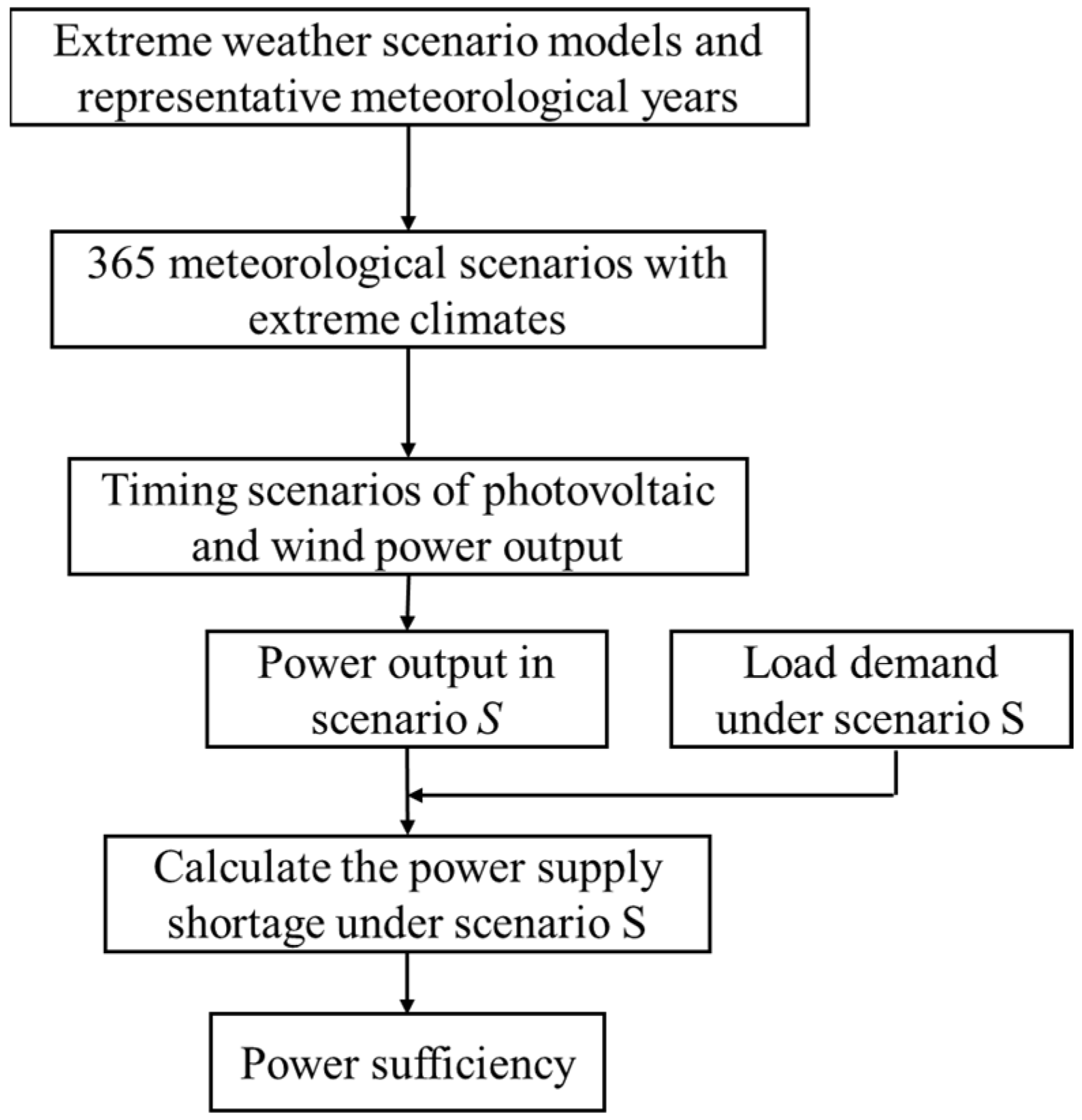
First, utilizing the extreme weather scenario model and meteorological data generated from typical meteorological years, a comprehensive meteorological dataset encompassing extreme weather months is constructed, resulting in 365 distinct meteorological scenarios representing the entire year.

$$S=\left\{\begin{array}{c}\mathrm{Rainy} \mathrm{season} \mathrm{and} \mathrm{hurricanes} \\ \mathrm{Typical} \mathrm{meteorological} \mathrm{days}\end{array}\right.$$

(15)

Step two involves integrating a renewable energy output model that accounts for climatic parameter influences to generate temporal scenarios for photovoltaic and wind power outputs.

Photovoltaic output:

$$P_{PV,S}={\displaystyle \sum _{T=1}^{24}\frac{1}{1000}{r}_T{P}_{PVN}\left[1-0.005(T_T-25 °\mathrm{C})\right]}$$

(16)

where $P_{PV,S}$ represents the power output of the photovoltaic system under scene S; $r_T$ denotes the real-time solar irradiance; $T_T$ indicates the ambient temperature; $P_{PVN}$ is the rated power for photovoltaic systems.

Wind power output:

$$P_{w,S}={\displaystyle \sum _{T=1}^{24}\frac{\pi }{8}\rho D^3{C}_P{V}_T^3}$$

(17)

where $P_{W,S}$ represents the power output of the wind turbine under scenario S; $V_T$ denotes the ambient wind speed in real-time conditions; $D$ is the diameter of the fan blades; $C_P$ is the wind energy utilization efficiency.

4. A Multi-Temporal and Multi-Spatial Power Supply Planning Model Considering Generation Capacity Adequacy

When extreme weather events occur, renewable energy generation experiences significant fluctuations due to climate variability, threatening the safety of power supply and demand within the electrical grid. This study utilizes a set of renewable energy output scenarios based on typical meteorological years to calculate the grid’s generation adequacy and assess the reliability of power supply. Additionally, a multi-temporal and multi-spatial power supply planning model that incorporates generation adequacy considerations is developed to optimize the capacity and siting of power sources such as photovoltaic, wind, thermal, and energy storage systems.

4.1. Methodology for Calculating Power Generation Adequacy Under Extreme Weather Scenarios

The occurrence of extreme weather events significantly reduces the reliability of power system supply. This paper employs a typical meteorological year-based method to generate renewable energy output scenarios, resulting in 365 weather scenarios. Subsequently, using a renewable energy output model influenced by climate parameters, the total power generation is calculated. Based on the overall grid load, the electricity shortage for each scenario is determined, thereby characterizing the power supply adequacy [24]. The calculation logic for power generation adequacy under extreme weather scenarios is illustrated in Figure 2.

The following outlines the steps for calculating the power generation adequacy:

(1)

Calculation of electricity shortage in Scenario S:

$$EEN{S}_S={\displaystyle \sum _{T=1}^{24}\max \left(L_{T,S}-P_{total,T,S},0\right)}$$

(18)

where $L_{T,S}$ represents the load at time T under scenario S; $P_{total,T,S}$ denotes the total power output of the power source at time T under scenario S.

(2)

Global power deficiency:

$$EENS={\displaystyle \sum _{S=1}^{365}EEN{S}_S}$$

(19)

4.2. Power Supply Planning Model

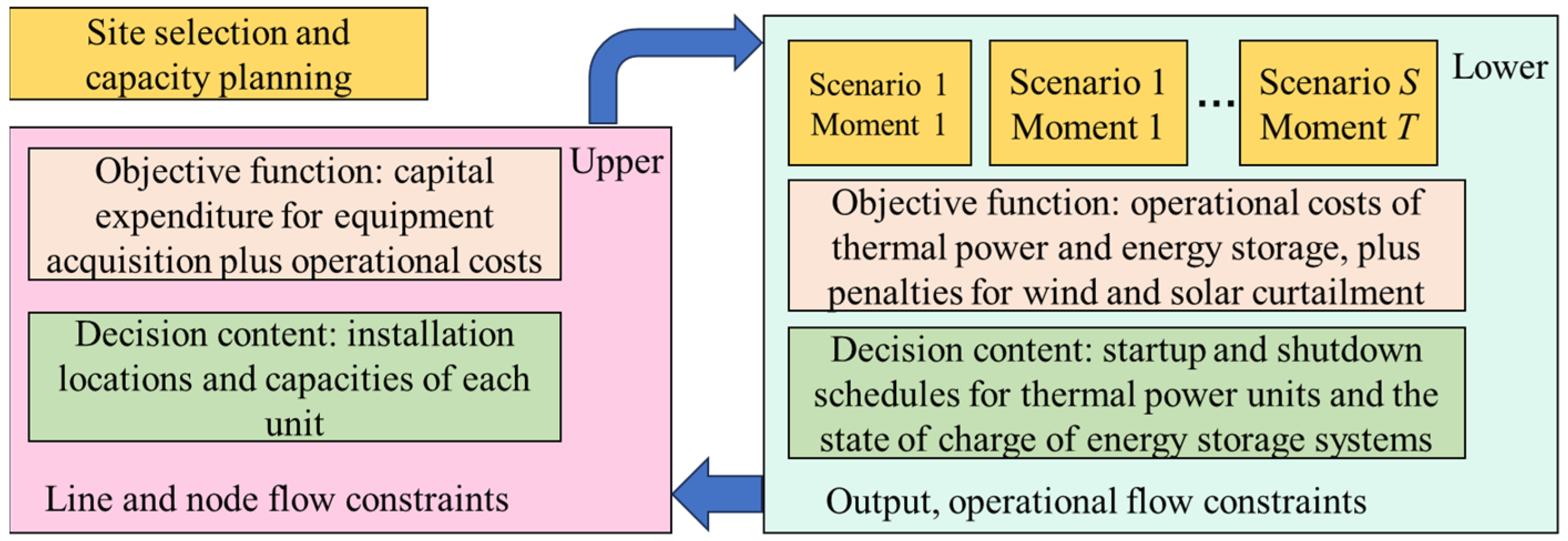
During instances of load shedding due to power shortages or outages, the power system implements reliability assurance measures to reduce the rate of load loss. Typically, this involves activating backup power sources or disconnecting tertiary loads and less critical secondary loads to alleviate supply pressure. This paper establishes a two-stage reliability assurance power source planning model, utilizing a capacity allocation and site selection approach to determine the optimal locations and capacities for photovoltaic, wind, thermal, and energy storage units. Based on this framework, the model further optimizes the dispatch of thermal and energy storage units to ensure the continuous and reliable operation of the power system. The structural framework of the two-stage planning model is shown in Figure 3.

4.2.1. Site Selection and Capacity Determination Model

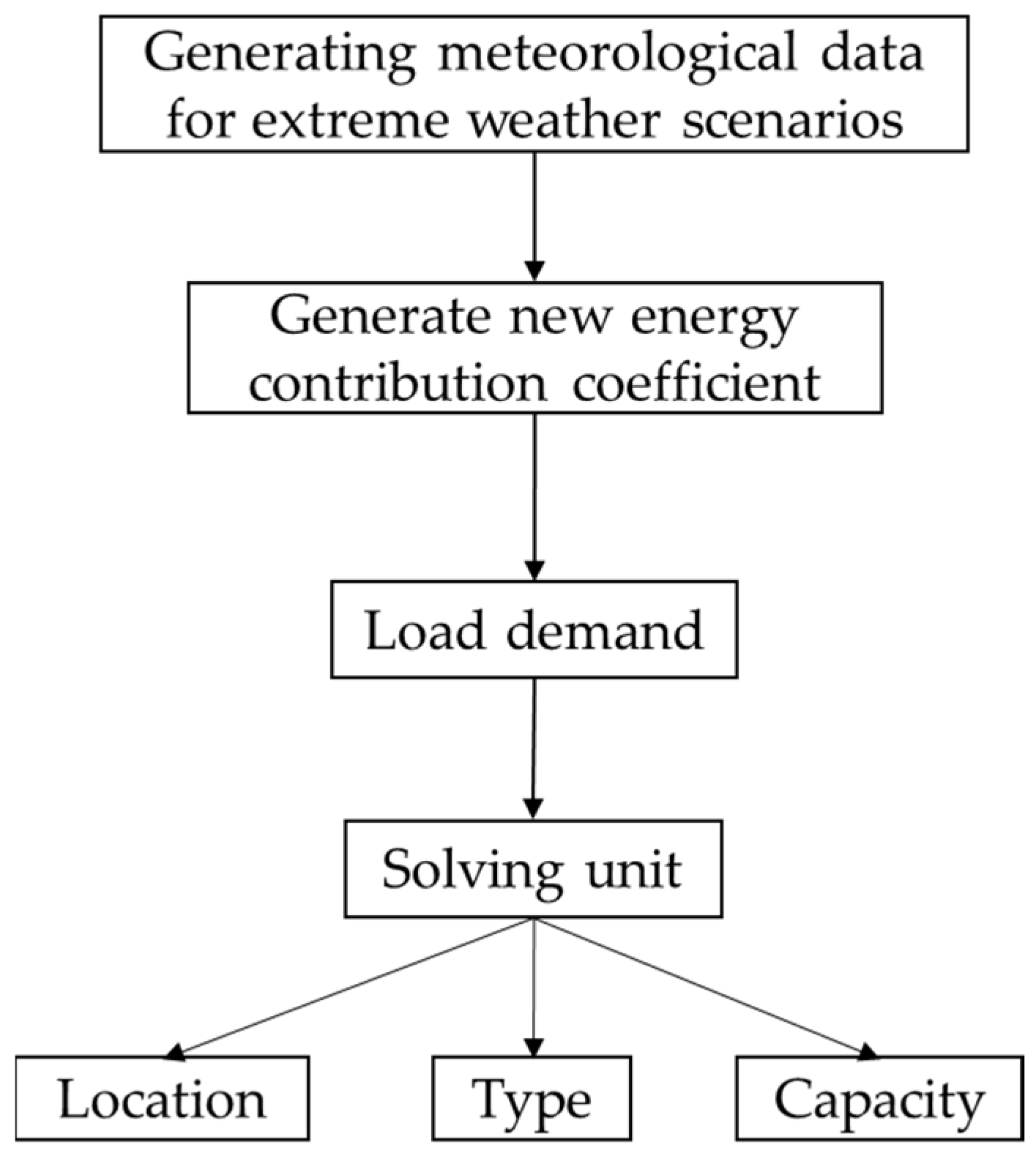
The siting and capacity determination model aims to minimize the total investment and operational costs. It employs binary 0–1 variables for site selection, as well as decision variables including the installed capacity of each generator unit, the real-time power output of each unit, and the charging and discharging power of energy storage systems. Constraints are imposed to ensure power balance, generator output limits, ramp rate restrictions, energy storage charging and discharging constraints, as well as power flow constraints on transmission lines and nodes. The detailed formulation process of the siting and capacity determination model is as follows:

(1) 

Decision Variables

(1) Binary site selection variables:

$$x_i^j\in \left\{0,1\right\}$$

(20)

where $x_i^j$ represents the site selection variables for photovoltaic, wind power, thermal power, and energy storage systems. Specifically, they indicate whether a power source of type j is installed at node i, with a value of 0 denoting the absence of installation and a value of 1 indicating the presence of the installation.

(2) Installed capacity:

$$P_i^j\ge 0$$

(21)

where $P_i^j$ represents the capacity of photovoltaic, wind power, thermal power, and energy storage installed at node i for each respective power source; its value should be greater than or equal to zero. If no such power source is installed at the node, the value is zero.

(3) Real-time power output:

$$P_{i,t}^j\ge 0$$

(22)

where $P_{i,t}^j$ represents the real-time power output of photovoltaic, wind, and thermal power units; due to weather conditions and unit startup and shutdown schedules, the real-time output may be zero.

(4) Energy storage charging and discharging:

$$\begin{array}{l}0\le P_{i,t}^{ESS,ch}\le P_{i,t,\max }^{ESS,ch}\\ 0\le P_{i,t}^{ESS,dis}\le P_{i,t,\max }^{ESS,dis}\end{array}$$

(23)

where $P_{i,t}^{ESS,ch}$ and $P_{i,t}^{ESS,dis}$ represent the energy storage charging and discharging power at time t, respectively, both of which must not exceed the maximum allowable charging and discharging power during the charge–discharge cycle.

(2) 

Objective Function

In the capacity planning and site selection model, the total cost primarily encompasses the procurement cost of the generating units and the operational and maintenance costs incurred during their daily operation.

(1) Minimize equipment procurement and operational maintenance costs:

$$\min f=\min \left(f_1+f_2\right)$$

(24)

(2) Equipment acquisition cost:

$$f_1={\displaystyle \sum _{i,j}{C}_1^j\times P_i^j}$$

(25)

where $C_1^j$ represents the procurement cost of equipment with unit capacity for different power source types.

(3) Operational and maintenance costs:

$${\displaystyle \sum _{i,j}{C}_2^j\times P_{i,t}^j}$$

(26)

where $C_2^j$ represents the operational and maintenance costs per unit capacity for different power source types.

(3) 

Constraint Conditions

(1) Power Balance:

$${\displaystyle \sum _i\left(P_{i,t}^G+P_{i,t}^{PV}+P_{i,t}^W+P_{i,t}^{ESS,dis}\right)}={\displaystyle \sum _i\left(L_{i,t}+P_{i,t}^{ESS,ch}\right)}$$

(27)

Equation (27) indicates that at each moment, the real-time power output of photovoltaic, wind, and thermal power units, along with the energy storage discharge power, satisfies the load and energy storage charging requirements. In this context, energy storage discharge is regarded as a power source output, while charging is considered as a load.

(2) Output limitations of photovoltaic and wind power units:

$$\begin{array}{l}0\le P_{i,t}^{PV}\le x_i^{PV}·P_i^{PV}·{\eta }^{PV}\\ 0\le P_{i,t}^W\le x_i^W·P_i^W·{\eta }^W\end{array}$$

(28)

Equation (28) indicates that the power output of photovoltaic and wind power systems cannot exceed their respective installed capacities; ${\eta }^{PV}$ and ${\eta }^W$ represents the conversion efficiencies of photovoltaic and wind power.

(3) Energy Storage Constraints:

$$\begin{array}{c}ES{S}_{i,t+1}=ES{S}_{i,t}+\left({\eta }^{ch}{P}_{i,t}^{ESS,ch}-{\displaystyle \frac{P_{i,t}^{ESS,dis}}{{\eta }^{dis}}}\right)\Delta t\\ 0\le ES{S}_{i,t}\le x_i^{ESS}·P_i^{ESS}\end{array}$$

(29)

where the ESS at time t + 1 equals the ESS at time t plus the charging amount of energy stored at time t minus the discharging amount at time t, with the constraint that the ESS capacity at each time step does not exceed the installed energy storage capacity.

(4) Mutual exclusivity of energy storage charging and discharging:

$$P_{i,t}^{ESS,ch}·P_{i,t}^{ESS,dis}=0$$

(30)

Equation (30) indicates that the energy storage system cannot simultaneously charge and discharge within the same time period.

(5) Constraints on thermal power plant unit output:

$$P_{i,\min }^G\le P_{i,t}^G\le P_{i,\max }^G$$

(31)

Equation (31) indicates that the thermal power plant’s output should operate within specified limits to prevent prolonged overload or light-load operation, which could damage equipment and result in economic losses.

(6) Ramp rate constraints for thermal power units:

$$\left|P_{i,t}^G-P_{i,t-1}^G\right|\le \Delta P_{i,\max }^G$$

(32)

The ramping constraint is a critical limitation on the output adjustment rate of thermal power units, specifying the maximum permissible change in power output between consecutive time intervals to prevent rapid fluctuations that could lead to the accumulation of mechanical stress and subsequent equipment damage.

(7) Transmission line flow constraints:

$$\left|P_{ij,t}\right|=\left|{\displaystyle \frac{{\theta }_{i,t}-{\theta }_{j,t}}{X_{ij}}}\right|\le P_{ij}^{\max }$$

(33)

In Equation (33), ${\theta }_{i,t}$ and ${\theta }_{j,t}$ represent the voltage phase angle at nodes i and j at time t; $X_{ij}$ represents the reactance of line ij.

The line power flow constraints are implemented to ensure that the power transmission does not exceed the designed capacity of the transmission lines, thereby preventing equipment damage and blackouts caused by line overloads.

(8) Node power flow constraints:

$${\displaystyle \sum _{m\in {{\rm N}}_i}{P}_{mi}+P_{i,t}^j}=L_i+{\displaystyle \sum _{k\in {{\rm N}}_i}{P}_{ik}}$$

(34)

where $P_{mi}$ represents the power flow from the downstream node m to node i; $P_{i,t}^j$ denotes the power output of the generators installed at node i; $L_i$ indicates the total load at node i; $P_{ik}$ signifies the power flow from node i to node k; and $N_i$ is the set of nodes directly connected to node i. The solution process of the site selection and capacity determination model is shown in Figure 4.

4.2.2. Unit Configuration Model

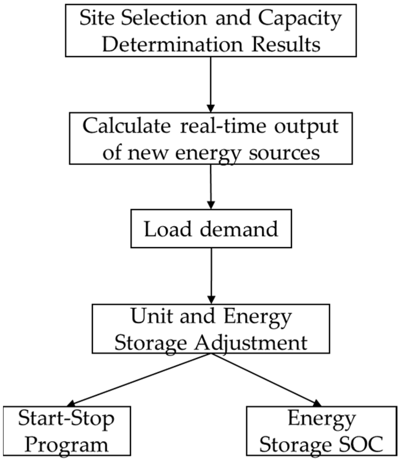
Using the total operating cost as the objective function, the optimization model for unit commitment is solved to determine the startup and shutdown schedule of thermal power units and the state of charge of energy storage systems.

(1) 

Decision Variables

This section introduces a binary variable, $u_{i,t}\in \left\{0,1\right\}$, to represent the on/off status of generating units. Variable $u_{i,t}$ equals 0 when the thermal power unit at node i is in a shutdown state at time t, and 1 when it is operational. Additionally, the real-time power outputs of each unit are defined: $P_{i,t}^G$ for thermal power units; $P_{i,t}^{PV},P_{i,t}^W$ for photovoltaic and wind power generation; $P_{i,t}^{ESS,ch},P_{i,t}^{ESS,dis}$ for charging/discharging power of the energy storage system at time t; $SO{C}_{i,t}$ for the state of charge of the energy storage system at time t; and $P_{i,t}^{curt}$ for the curtailed wind and solar power resulting from insufficient absorption capacity.

(2) 

Objective Function

The model incorporates the startup and shutdown of thermal power units as well as the charging and discharging of energy storage systems. Consequently, the total cost comprises the fuel costs associated with thermal power operation and the operational and maintenance costs of energy storage. Additionally, it accounts for the startup and shutdown costs of the units and penalties for wind and solar power curtailment. These costs constitute the overall objective function of the model.

Minimize the total operational cost:

$$\min \left({\mathrm{w}}_1{+\mathrm{w}}_2{+\mathrm{w}}_3\right)$$

(35)

Start-up, shutdown, and operational maintenance costs of thermal power units:

$${\displaystyle \sum _{i,t}\left(C^{fuel}{P}_{i,t}^G+C^{su}{u}_{i,t}\left(1-u_{i,t-1}\right)\right)}$$

(36)

where $C^{fuel}$ represents the fuel cost per unit capacity of the thermal power unit; $C^{su}$ denotes the startup and shutdown costs of the thermal power unit.

Operational and maintenance costs of energy storage systems:

$${\displaystyle \sum _{i,t}\left(C^{ESS}\left(P_{i,t}^{ESS,ch}+P_{i,t}^{ESS,dis}\right)\right)}$$

(37)

where $C^{ESS}$ represents the operational and maintenance costs per unit capacity of energy storage.

The costs associated with penalties for abandoning wind and solar energy sources:

$${\displaystyle \sum _t{C}^{curt}{P}_t^{curt}}$$

(38)

where $C^{curt}$ represents the unit penalty cost for wind and solar power curtailment.

(3) 

Constraint Conditions

(1) Power Balance (Reliability Assurance):

$${\displaystyle \sum _{i\in G}{P}_{i,t}^G}+{\displaystyle \sum _{i\in PV}{P}_{i,t}^{PV}}+{\displaystyle \sum _{i\in W}{P}_{i,t}^W}+{\displaystyle \sum _{i\in ESS}{P}_{i,t}^{ESS,dis}}={\displaystyle \sum _{i\in N}{L}_{i,t}}+{\displaystyle \sum _{i\in ESS}{P}_{i,t}^{ESS,ch}}$$

(39)

(2) Constraints of thermal power units:

According to the installation and capacity settings of thermal power units, output restrictions are established.

$$u_{i,t}{P}_i^{\min }\le P_{i,t}^G\le u_{i,t}{P}_i^{\max }$$

(40)

where $P_i^{\min }$ and $P_i^{\max }$ represent the minimum and maximum output power.

Rapid ramping can adversely affect generator equipment and grid frequency, exacerbating equipment wear, increasing maintenance costs, and potentially compromising safety and operational integrity.

$$\begin{array}{l}\mathrm{ascending} \mathrm{the} \mathrm{incline} :P_{i,t}^G-P_{i,t-1}^G\le \Delta P_i^{up}\\ \mathrm{descending} \mathrm{the} \mathrm{incline}:P_{i,t-1}^G-P_{i,t}^G\le \Delta P_i^{down}\end{array}$$

(41)

where $\Delta P_i^{up}$ and $\Delta P_i^{down}$ represent the maximum ascent and descent slopes, respectively.

(3) To prevent frequent start-stop cycles of the equipment and to extend its operational lifespan, constraints are imposed on the timing of unit startups and shutdowns.

$$\left\{\begin{array}{c}{u}_{i,t}-u_{i,t-1}\le u_{i,t+ton-1}\\ u_{i,t-1}-u_{i,t}\le 1-u_{i,t+toff-1}\end{array}\right.$$

(42)

where $u_{i,t+ton-1}$ and $u_{i,t+toff-1}$ represent the minimum up and down times of the generating unit, respectively. When the unit transitions from a shutdown state to an operational state at time t, the condition $u_{i,t+ton-1}=1$ must be satisfied, indicating that the unit must remain in the operational state for at least ton − 1 time intervals prior to t. This reflects the requirement that the start-up and shutdown processes of thermal power units adhere to specific temporal constraints. The solution process of the unit combination model is shown in Figure 5.

5. Case Study Analysis

This study utilizes the IEEE 24-bus system as a case example. Initially, the impact scope of extreme weather events is determined based on the monsoon and hurricane scenario models. Typical meteorological years are generated using the Finkelstein–Schafer statistical method, followed by optimal site selection, capacity sizing, and unit combination optimization for the IEEE 24-bus system. Analysis of renewable energy output and its correlation with climatic factors, utilizing data from the North Dakota Agricultural Weather Network [25]. The power system’s adequacy is evaluated by selecting the power shortage as the key performance indicator, considering the total power output and load demand.

5.1. Solution of Extreme Weather Scenario Models

5.1.1. The Rainy Season

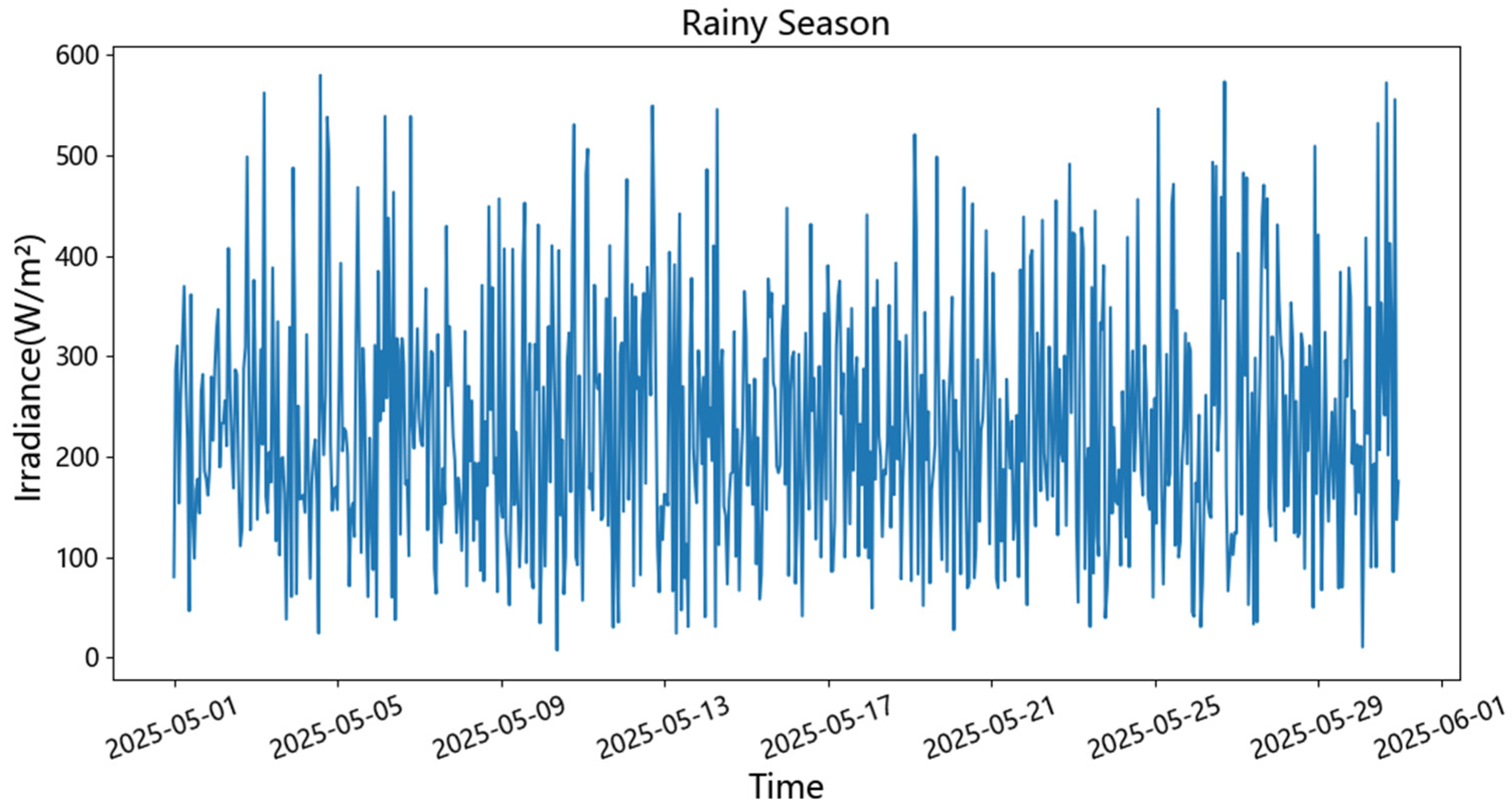
To account for the spatiotemporal effects of the IEEE 24-bus system model, the analysis of the upper region’s geographical characteristics reveals low rainfall intensity, prolonged duration, and a rainfall intensity threshold set at 12 mm/h. Conversely, the lower region exhibits higher rainfall intensity, increased variability, and an elevated rainfall threshold of 20 mm/h. By adjusting the empirical attenuation parameters and Weibull distribution parameters, irradiance models for the upper, middle, and lower regions were derived, with region-specific parameter values detailed in

Table 3. Different region parameter values.

Parameter		Upper	Central	Lower
Weber	β	1.0	1.2	1.5
Distribution	η	3.0	4.0	5.0
Experience	a	0.15	0.18	0.22
Parameters	b	0.5	0.6	0.7

. Figure 6. presents the irradiance data obtained under typical parameter settings for the central region. The analysis indicates a significant reduction in irradiance during the rainy season, which adversely affects photovoltaic power generation.

5.1.2. Hurricane Conditions

Based on the hurricane spatiotemporal evolution model, the hurricane’s trajectory is determined. In analyzing the affected area, this study assigns coordinate values to the IEEE 24-node system within a 100 × 100 grid, facilitating the calculation of distances from the hurricane center to delineate the impact zone.

Table 4. Partial node coordinate values.

Node	1	2	17	18
Coordinate	(15, 90)	(35, 85)	(10, 50)	(50, 90)

presents the coordinates of selected nodes:

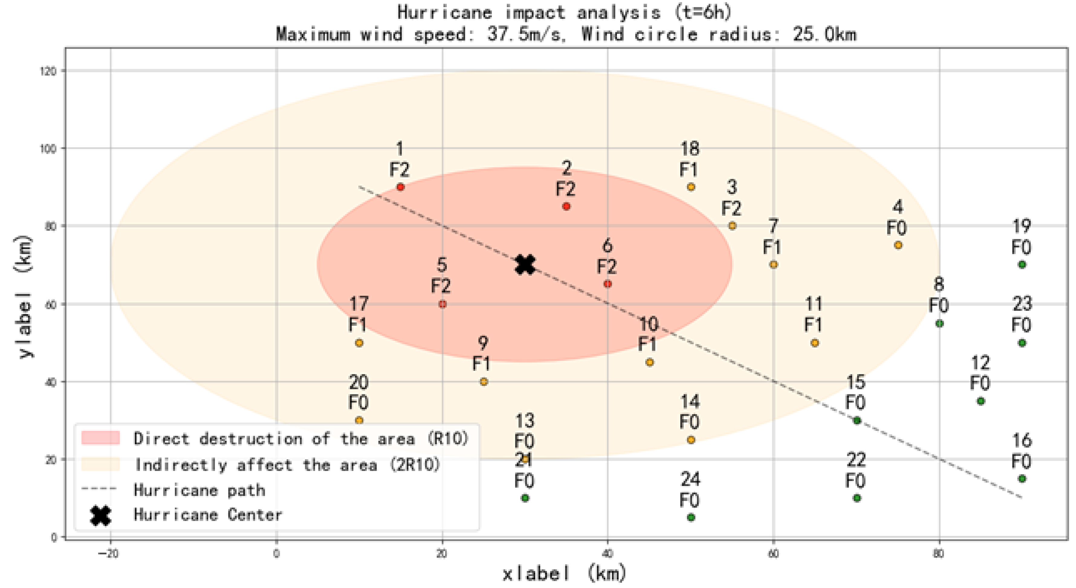
During the hurricane’s progression, the impact on each system node varies dynamically over time and space. The maximum wind speed and the radius of the wind circle decrease as time progresses, leading to a contraction of the affected area. This temporal evolution during the six-hour hurricane impact period is illustrated in Figure 7.

Calculate the position of the hurricane’s center and wind speed, and determine the distances between the center and each node. Assess the impact type and wind speed at each node. The affected degree and wind speed data for each node at the 12th hour of the hurricane are presented in

Table 5. T = 12 h, each node is affected by hurricane and wind speed.

Node	Distance (km)	Types of Influence	Wind Speed (m/s)	Node	Distance (km)	Types of Influence	Wind Speed (m/s)
1	53.2	Safety	12.5	13	36.1	Indirect	13.4
2	38.1	Indirect	12.1	14	25.0	Indirect	23.4
3	30.4	Indirect	17.8	15	28.3	Indirect	19.8
4	35.4	Indirect	13.9	16	53.2	Safety	12.9
5	31.6	Indirect	16.8	17	40.0	Indirect	11.0
6	18.0	Direct	29.8	18	40.0	Indirect	10.9
7	22.4	Indirect	26.7	19	44.7	Safety	12.8
8	30.4	Indirect	17.8	20	44.7	Safety	11.6
9	26.9	Indirect	21.2	21	44.7	Safety	12.3
10	7.1	Direct	30.5	22	44.7	Safety	12.6
11	15.0	Direct	30.2	23	40.0	Indirect	11.6
12	38.1	Indirect	12.1	24	45.0	Safety	13.1

.

When the cut-in wind speed of wind turbine is 3 m/s and the cut-out wind speed is 25 m/s, under a sustained hurricane for 12 h, both the wind speed at the hurricane’s center and the radius of the 10-level wind circle decrease, resulting in a reduction in the number of affected nodes.

5.2. Composition of a Typical Meteorological Year

An examination of meteorological literature on the East Asian rainy season and hurricanes reveals that the rainy season predominantly occurs in May, while hurricanes are more frequent during the summer months. Consequently, May and July are designated as the months representing extreme weather conditions. Non-extreme weather months are determined using a decade of historical data from 2007 to 2016, analyzed via the Finkelstein–Schafer statistical method. Extreme weather months are modeled based on scenarios of extreme rainy season and hurricane events. The composition of a typical meteorological year is summarized in

Table 6. Composition of a typical meteorological year.

Month	1	2	3	4	5	6
Data	2012.1	2009.2	2012.3	2014.4	Rainy season	2008.6
Month	7	8	9	10	11	12
Data	Hurricane	2012.8	2007.9	2011.10	2011.11	2015.12

.

5.3. Solution of the Site Selection and Capacity Determination Model

The site selection and capacity determination model involves solving for the installation locations and capacities of each generating unit. The objective is to minimize the total system cost while satisfying power balance constraints, as well as nodal and transmission line flow restrictions, thereby establishing the optimal installation scheme for each node.

In the site selection and capacity allocation plan, renewable energy installations account for approximately 1670 MW, representing about 50% of the total installed capacity. Concurrently, the system incorporates 780 MW of energy storage to facilitate energy absorption and supply security. This configuration exemplifies a high proportion of renewable energy integration; additionally, considering the impact of extreme weather conditions on renewable output, the capacity of thermal power and energy storage units has been increased to ensure reliable power supply.

As detailed in

Table 7. The results of the site selection and capacity model.

Node	PV	Wind	Thermal	Energy Storage	Node	PV	Wind	Thermal	Energy Storage
1			200	50	13	100			50
2	100			50	14	100	50		50
3	100	100		50	15				50
4	100				16		20		50
5	100			50	17	100			50
6			200	50	18
7		100	200	50	19			200
8				50	20	100			50
9					21		100	200
10	100	100	200	50	22	100
11				50	23			200
12	100		100	50	24	100

, nodes equipped with photovoltaic and wind power installations tend to reduce the installed capacity of thermal units and are supplemented with appropriate energy storage systems, such as nodes 2, 3, 4, and 5. Conversely, nodes without renewable installations exhibit increased capacities for thermal units and energy storage, exemplified by nodes 1, 8, 11, and 15. Based on power flow constraints and nodal load demands, some nodes may omit unit installations altogether or install all available units, as observed in nodes 9 and 10.

5.4. Solution of the Unit Combination Model

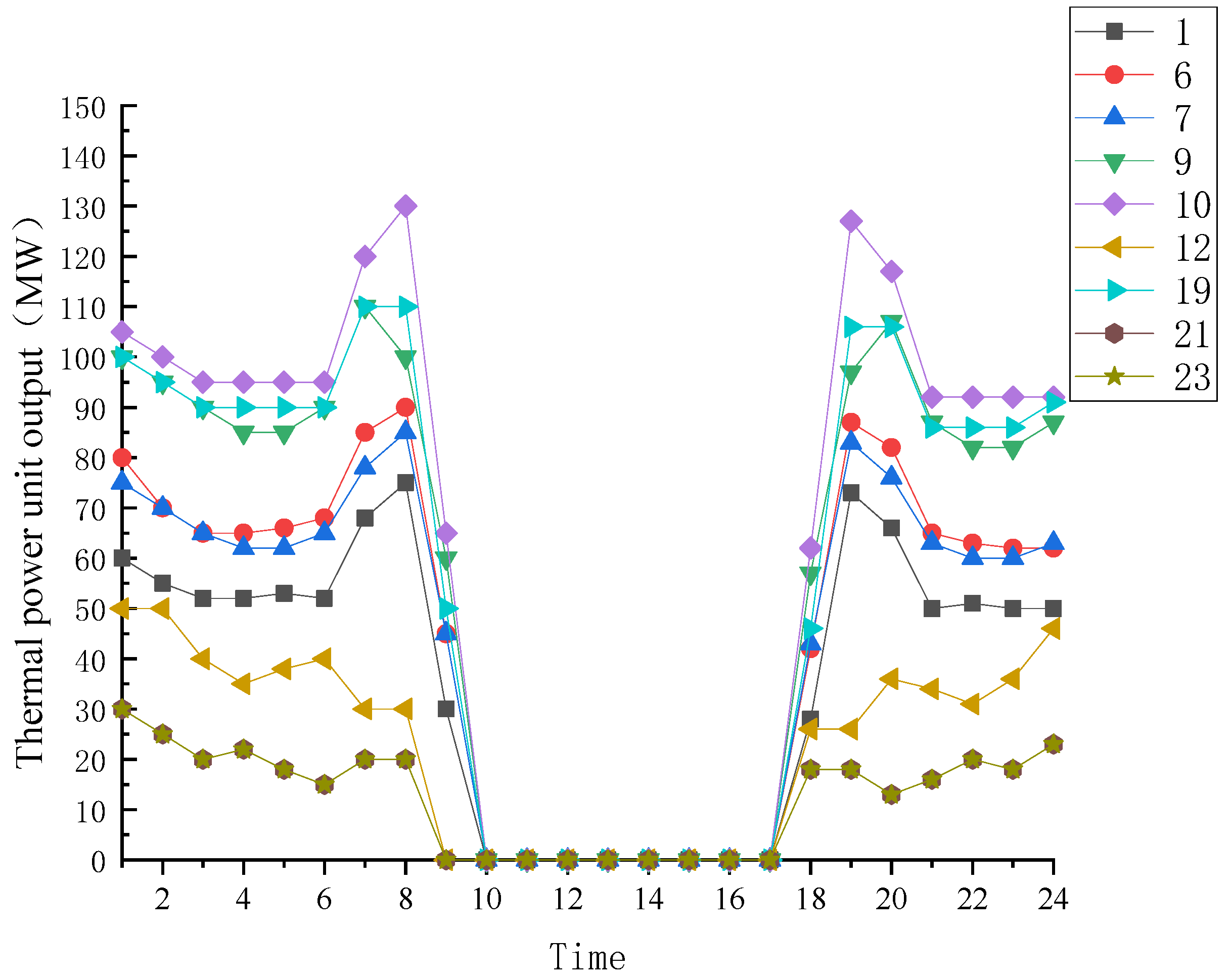
Solving the combined unit model yields the on/off status of thermal power units and the State of Charge (SOC) of energy storage over 8760 h. To reflect the impact of meteorological variations between typical and extreme weather months, the study performs simultaneous calculations for the same time periods in both typical and extreme months, resulting in the on/off status of thermal units and the SOC of energy storage. Figure 8 illustrates the power output of thermal units during typical months, while

Table 8. Typical month under the energy storage system SOC.

Node	Charging Power	Discharge Power	SOC
1	0	10	0.6
2	0	0	0.8
3	0	20	0.4
5	20	0	0.8
6	0	10	0.6
7	10	0	0.8
8	0	20	0.4
10	20	0	0.8
11	10	0	0.6
12	30	0	1
13	0	20	0.4
14	0	0	0.8
15	0	20	0.67
16	0	0	0.6
17	20	0	1
20	10	0	0.8

Note: The output and charging/discharging power units in the table are expressed in MW.

presents the results of the energy storage SOC status under typical month conditions.

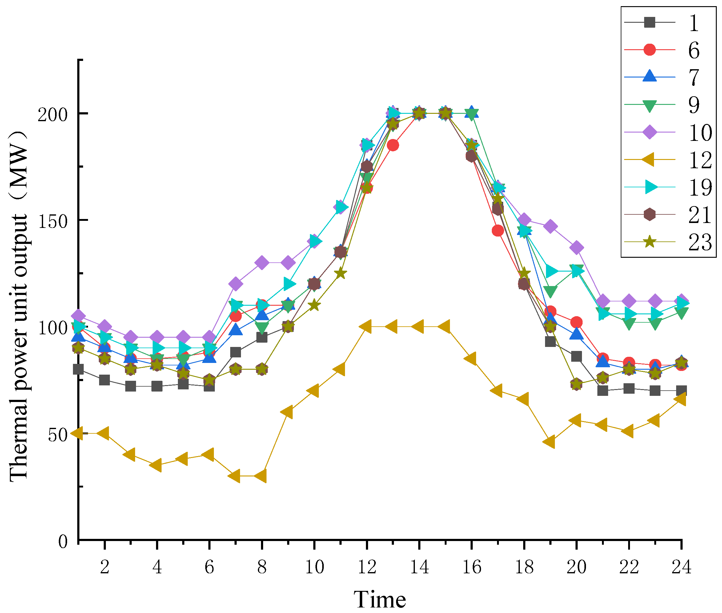
By selecting the time periods with the highest proportion of solar and wind power output, it is evident from the table data that most thermal power units are in a shutdown state, with only some nodes operating under higher loads to supply power to the load. Regarding the State of Charge (SOC) of the energy storage system, the majority of storage units are charging, indicating the process of absorbing renewable energy output. During extreme months, renewable energy output is significantly affected by climate variability, resulting in fluctuations that pose substantial threats to the reliable operation of the power system. Figure 9 illustrates the power output curves of thermal units during these extreme months, while

Table 9. SOC of energy storage system in extreme months.

Node	Charging Power (MW)	Discharge Power (MW)	SOC
1	13	0	0.46
2	0	40	0.2
3	0	50	0
5	0	20	0.6
6	15	0	0.6
7	10	0	0.3
8	0	40	0.2
10	0	10	0.2
11	0	20	0.4
12	0	30	0.2
13	0	30	0.2
14	0	8	0.2
15	0	20	0.33
16	0	20	0.4
17	10	0	0.6
20	0	10	0.4

presents the SOC calculation results of the energy storage system under the same conditions.

When compared to the same periods in typical months, all thermal power units operate at full capacity during extreme weather conditions, with the majority of energy storage systems functioning as backup power sources to supply the load. This indicates that under extreme weather scenarios, when renewable energy output is significantly reduced, thermal power plants and energy storage systems bear the majority of the load demand.

5.5. Power Supply Adequacy

In the context of extreme weather scenarios, the generation adequacy of the power system can be evaluated through the following steps: firstly, calculating the total power output and load demand for each time period based on typical meteorological year data, thereby determining the energy shortfall; secondly, performing a time-weighted summation of the energy shortfalls across all scenarios to obtain the overall supply deficit. A smaller supply deficit indicates a higher generation capacity and greater stability of power supply under extreme weather conditions.

This study presents selected time points, as shown in

Table 10. There is a shortage of power supply in different scenarios.

Scenario	Time	Lack of Power Supply (MWh)
Typical	09:00–12:00	1.37
Extreme	09:00–12:00	15.56
Typical	18:00–21:00	3.32
Extreme	18:00–21:00	25.81

, where the total global supply deficit is calculated to be 46.05 MWh.

5.6. Economic Analysis

By solving the two-stage power supply planning model, the total investment cost and total annual operation and maintenance cost are obtained as follows:

• Total Investment Cost: 2670 million yuan
• Total Annual Operation and Maintenance Cost: 52.95 million yuan/year

From an initial investment perspective, power generation facility construction costs represent the primary expenditure. These include procurement and installation expenses for photovoltaic and wind power equipment; thermal power plant construction involves high costs for units and environmental protection equipment; energy storage systems require substantial initial capital due to the high cost of batteries and management systems. During the operation and maintenance phase, routine maintenance costs for photovoltaic and wind power facilities remain relatively stable, but equipment failure rates increase following extreme weather events, leading to higher maintenance expenses. Fuel and environmental compliance costs for thermal power fluctuate significantly due to market and policy influences; battery replacement costs constitute a high proportion of energy storage expenses. However, from an overall economic perspective: Enhancing power supply reliability reduces substantial economic losses for industrial and commercial users caused by outages; Integrating renewable energy aligns with policy objectives while generating revenue from electricity sales and green certificate trading; Energy storage and thermal power plants participating in peak shaving and frequency regulation markets can earn corresponding compensation according to market trading rules.

6. Conclusions

This paper addresses the supply security risks in power systems induced by extreme weather events under high penetration of renewable energy sources. A multi-temporal and spatial power supply planning method integrating the spatiotemporal evolution characteristics of extreme weather is proposed. By establishing models for radiation attenuation during the rainy season and the spatiotemporal evolution of hurricane paths, this study quantifies the impacts of extreme weather on renewable energy output and grid equipment, highlighting their spatial and temporal variability. Combining a power output model incorporating climate parameters with typical meteorological year data generated via the Finkelstein–Schafer method, a two-stage power supply planning model based on generation adequacy is developed. This model facilitates the coordinated siting; capacity allocation; and optimal dispatch of thermal, energy storage, and renewable sources. Simulations conducted on the IEEE 24-bus system, considering terrain and spatial heterogeneity in extreme weather scenarios of the rainy season and hurricanes, validate and analyze the proposed planning approach. The main conclusions are summarized as follows:

(1)

During rainy season, the irradiance significantly decreases, resulting in a substantial reduction in photovoltaic output; under hurricane conditions, wind speeds at certain nodes exceed the cut-out wind speed of 25 m/s, causing wind turbines to shut down and severely limiting renewable energy generation. Quantitatively, photovoltaic generation decreased by up to 35% during the rainy season, while approximately 20% of wind turbines reached the cut-out threshold under hurricane conditions. The case study results indicate that under extreme weather conditions, thermal power units operate near full capacity, while energy storage systems predominantly discharge, assuming the primary supply role and effectively mitigating the power supply gap caused by insufficient renewable output.

(2)

The planned system exhibits a total power deficiency of 46.05 MWh under extreme weather scenarios. Although this exceeds the typical daily scenario, optimized coordination of thermal power and energy storage significantly reduces the impact of extreme weather on the system’s power supply capacity.

(3)

From a practical perspective, the proposed framework provides actionable guidance for system planners to allocate capacity among renewable, thermal, and storage units under varying meteorological conditions. It enables risk-informed planning that quantitatively links climate variability with power supply reliability, supporting investment decisions in climate-sensitive regions.

(4)

Future research will extend the framework to include demand-side management, cyber-physical risk modeling, and long-term climate projection data (e.g., CMIP6) to further strengthen the adaptability and robustness of new power systems under evolving climatic uncertainty.

7. Limitations and Future Work

The proposed multi-spatiotemporal power source planning framework improves system resilience under extreme weather events; however, several limitations remain.

(1)

Model scope: Only plum rain and hurricane conditions are considered. Future work will extend to multiple climate hazards and long-term projections (e.g., CMIP6 datasets).

(2)

Demand-side integration: The current framework focuses on the supply side; future research will incorporate demand-side management and load flexibility to enhance system adaptability.

(3)

Cyber-physical resilience: The study assumes ideal control and communication conditions. Future work will include cyber-physical co-simulation to evaluate system robustness under communication failures.

(4)

Temporal and uncertainty scale: Typical Meteorological Year (TMY) data capture annual variability but not interannual climate trends. Future studies will employ long-term probabilistic climate scenarios.

(5)

Scalability: Validation was conducted on the IEEE 24-bus system. Future applications to regional or national grids will verify model scalability and practical value.

References

1. Li, M.-D.; Han, C.-F.; Meng, L.-P.; Liu, P.; Shao, Z. Spatiotemporal dynamics and driving factors of the coupling coordination between solar photovoltaic efficiency and installed capacity in China (2015–2023). Renew. Energy 2025, 247, 122991. [Google Scholar] [CrossRef]
2. Yang, Z.; Liu, D.; Zeng, X.; Fan, C.; Yang, X.; Huang, Y. Modelling and simulation study on dynamic pollution accumulation process of composite insulator. High Volt. 2024, 9, 601–603. [Google Scholar] [CrossRef]
3. Trakas, D.N.; Hatziargyriou, N.D. Resilience constrained day-ahead unit commitment under extreme weather events. IEEE Trans. Power Syst. 2019, 35, 1242–1253. [Google Scholar] [CrossRef]
4. Wu, Y.-J.; Xue, Y.-S.; Xie, Y.-Y.; Wang, H.; Duan, R.; Huang, W. Space-time Impact of Typhoon and Rainstorm on Power Grid Fault Probability. Autom. Electr. Power Syst. 2016, 40, 20–29. [Google Scholar]
5. Yang, Y.-H.; Tang, W.; Liu, Y.; Xin, Y.; Wu, Q. Quantitative resilience assessment for power transmission systems under typhoon weather. IEEE Access 2018, 6, 40747–40756. [Google Scholar] [CrossRef]
6. Liu, X.-N.; Hou, K.; Jia, H.-J.; Zhao, J.; Mili, L.; Jin, X.; Wang, D. A planning-oriented resilience assessment framework for transmission systems under typhoon disasters. IEEE Trans. Smart Grid 2020, 11, 5431–5441. [Google Scholar] [CrossRef]
7. Mohammad, R.; Mohsen, K. Improving the resilience of distribution network in coming across seismic damage using mobile battery energy storage system. J. Energy Storage 2022, 52, 104891. [Google Scholar] [CrossRef]
8. Li, J.; Wang, Z.; Da, Z.; Ren, Y.; Jin, Y.; Zhou, B. A Multi-level Planning Method for Energy Storage Stations in Flexible Distribution Networks Considering the Spatio-temporal Correlation of Severe Weather. Power Syst. Prot. Control 2023, 51, 128–137. [Google Scholar]
9. Liao, J.; Wang, R.; Xia, S.; Ren, L.; Wang, T. Joint planning of distribution network and electric vehicle charging station considering extreme weather events. J. Phys. Conf. Ser. 2022, 2276, 2276. [Google Scholar]
10. Xue, Y.-W.; Zhang, K.; Wang, Z.; Guo, G.; Liu, D.; Shi, R.; Huang, S. Planning of distributed energy storage with the coordination of transmission and distribution systems considering extreme weather. Front. Energy Res. 2024, 12, 1505582. [Google Scholar] [CrossRef]
11. Qin, J.-J.; Fang, F.; Tian, X. Optimization configuration of hybrid energy storage capacities for large-scale renewable energy bases in desert: A case study of Tennger, China. Energy 2025, 332, 136791. [Google Scholar] [CrossRef]
12. Shi, Z.; Yang, Z.; Zeng, X.; Zhou, J.; Pan, W.; Huang, Y. Modeling and application research of DC dynamic pollution flashover process based on insulator equivalent plate unfolding. Proc. CSEE 2025, 1–12. [Google Scholar] [CrossRef]
13. Yuan, J.-H.; Zhang, K.; Ding, B.-D.; Wei, H.; Zhang, J.; Mou, Q.; Peng, K.; Zhang, H. Enhancement strategy of power system resilience for supply-demand imbalance at extreme weather conditions: A high-share renewable energy case from Qinghai Province in China. Renew. Energy 2026, 256, 124048. [Google Scholar] [CrossRef]
14. Sun, W.-Q.; Huang, H.-F.; Chen, T.-W.; Wang, H. A two-stage source-load interaction power supply and demand matching method based on the ultra-high share of renewable power system. Sustain. Energy Grids Netw. 2025, 43, 101887. [Google Scholar] [CrossRef]
15. Zhou, L.-J.; Ye, B.; Xia, S.-Q. Assessing membrane biofouling and its gel layer of anoxic/oxic membrane bioreactor for megacity municipal wastewater treatment during plum rain season in Yangtze River Delta, China. Water Res. 2017, 127, 22–31. [Google Scholar] [CrossRef]
16. Li, H.-D.; Lou, S. Review of solar irradiance and daylight illuminance modeling and sky classification. Renew. Energy 2018, 126, 445–453. [Google Scholar] [CrossRef]
17. Li, Y.; The, J.-S.; Lai, C.-M. Assessing power grid vulnerability to extreme weather: The impact of electric vehicles and energy storage systems. J. Energy Storage 2025, 112, 115534. [Google Scholar] [CrossRef]
18. Liu, D.; Yang, Z.; Zeng, X.; Tang, T.; Fan, B.; Fan, C. Contamination deposition model of composite insulator surface based on discrete element analysis method. High Volt. Eng. 2024, 50, 2225–2236. [Google Scholar]
19. Chen, D.; Cai, Z.; Wu, H.; Guo, C. Review of distribution network’s resilience based on typhoon disaster. Energy Rep. 2022, 8 (Suppl. S16), 876–888. [Google Scholar] [CrossRef]
20. Pan, Y.; Zhao, W.; Xu, P.; Li, F.; Zhang, W.; Li, X. Construction of new energy output model and load probability model considering meteorological uncertainty. In Proceedings of the 2024 4th International Conference on New Energy and Power Engineering (ICNEPE), Guangzhou, China, 8–10 November 2024; IEEE: Piscataway, NJ, USA, 2024. [Google Scholar]
21. Marion, W.; Urban, K. User’s Manual for TMY2S: Typical Meteorological Years; National Renewable Energy Laboratory: Golden, CO, USA, 1995.
22. Zeng, Z.-Y.; Kim, J.-H.; Ralph, T.-M. An update to the Sandia method for creating Typical Meteorological Years from a limited pool of calendar years. Energy 2025, 320, 135143. [Google Scholar] [CrossRef]
23. GB/T 37526-2019; Method for Solar Energy Resource Assessment. China Standards Press: Beijing, China, 2019.
24. Peña, D.; Alexander, A.-T.; Francisco, J. Reliability Assessment of Ecuador’s Power System: Metrics, Vulnerabilities, and Strategic Perspectives. Energies 2025, 18, 3059. [Google Scholar] [CrossRef]
25. North Dakota Agricultural Weather Network. Weather Data. Available online: https://ndawn.info/index.html (accessed on 1 June 2025).
Figure 1. The impact of extreme weather on the source–grid–load side of the power system.
Processes 13 03385 g001
Figure 2. Generation adequacy calculation logic.
Processes 13 03385 g002
Figure 3. Two-tier planning framework.
Processes 13 03385 g003
Figure 4. Site selection and capacity determination model solution process.
Processes 13 03385 g004
Figure 5. Solution process for unit combination model.
Processes 13 03385 g005
Figure 6. Irradiance data during the rainy season.
Processes 13 03385 g006
Figure 7. The area of impact of the hurricane lasting 6 h.
Processes 13 03385 g007
Figure 8. Typical month under the thermal power unit output.
Processes 13 03385 g008
Figure 9. The power output of thermal power units during extreme months.
Processes 13 03385 g009