Spatiotemporal Modeling of the Total Nitrogen Concentration Fields in a Semi-Enclosed Water Body Using a TCN-LSTM-Hybrid Model

Abstract

In the field of water process engineering, accurately predicting the total nitrogen (TN) concentration distribution in the Semi-Enclosed Bay area is of great importance for water quality assessment, pollution control, and scientific management. Due to the coupling of multiple influencing factors, the pollution process is complex, and traditional monitoring methods struggle to achieve large-scale, long-term real-time observation. Although numerical simulations can reproduce TN transport processes, they are computationally expensive and have low prediction efficiency. To address this, this study develops a deep learning hybrid model that integrates a Temporal Convolutional Network (TCN) and a Long Short-Term Memory (LSTM) network, referred to as the TCN-LSTM-Hybrid Model, to predict the spatiotemporal distribution of TN concentration fields in Shenzhen Bay. Comparative experiments show that this model outperforms traditional models such as TCN, LSTM, GRU, and MLP in terms of prediction accuracy and spatial generalization, offering higher computational efficiency and breaking through the limitations of “point-based prediction” by achieving “field-based prediction,” thereby providing a new path for pollutant simulation in complex ocean environments, supporting more informed decision making in ocean and coastal management.

1. Introduction

In marine environments, pollution simulation and prediction play a crucial role in accurately understanding the diffusion and migration dynamics of pollutants in marine media, as well as in proactively planning and formulating effective marine pollution prevention strategies. In recent years, with the acceleration of urbanization and the intensification of human activities, water quality issues in bay areas have become increasingly prominent, particularly regarding the spatiotemporal variations in nitrogen pollutants, which urgently require in-depth research and scientific modeling [1]. However, this process is influenced by a combination of natural and anthropogenic factors [2], and the diffusion of pollutants exhibits highly nonlinear behavior. Traditional detection methods are time-consuming, labor-intensive, lack real-time monitoring capabilities, and offer limited spatial coverage [3]. Although Computational Fluid Dynamics (CFD) methods can reproduce pollutant transport in complex bay environments, they require precise initial and boundary conditions, incur high computational costs, and involve complex model construction and validation processes. Therefore, this study focuses on the simulation and prediction of total nitrogen (TN) concentrations in Shenzhen Bay and aims to achieve efficient forecasting through innovative methods.

In recent years, machine learning (ML) technologies have made significant progress across various fields. Their powerful data processing and pattern recognition capabilities make them effective tools for addressing complex problems [4,5,6,7,8]. Machine learning models can automatically learn patterns and features from large volumes of data, constructing models with high predictive capability. Deep learning, in particular, can extract implicit patterns from high-dimensional data through multiple layers of nonlinear transformations. For instance, convolutional neural networks (CNNs) are effective in capturing spatial heterogeneity, while recurrent neural networks (RNNs) and their variants are adept at handling temporal dependencies. These characteristics provide a new approach for modeling the spatial distribution and dynamic evolution of total nitrogen concentrations in Shenzhen Bay.

This study selects Shenzhen Bay, a typical highly urbanized bay, as the research area. As a core ecological corridor in the Guangdong–Hong Kong–Macao Greater Bay Area and a key node for integrated land–sea pollution control, Shenzhen Bay is facing serious total nitrogen exceedance issues, which directly impact the ecological security of the Pearl River Estuary and regional sustainable development. Thus, effectively predicting and managing TN concentrations in this region is of urgent practical importance. Additionally, the complex environmental characteristics of Shenzhen Bay, such as intricate hydrodynamic conditions and diverse pollution sources, make it an ideal case study to validate the application potential of deep learning techniques in environmental science. This case can not only provide strong support for water quality management and protection in the Shenzhen Bay area but also offer valuable practical experience for the broader application of deep learning in environmental studies.

Traditional experimental measurement techniques provide foundational methodological support for monitoring TN concentrations in water bodies. Bachmann et al. [9] proposed a novel method for determining TN in natural waters and found it to be more sensitive and accurate compared to the USEPA method. Ebina et al. [10] developed a method using persulfate oxidation to simultaneously determine TN and total phosphorus (TP) in water samples, improving detection efficiency. A series of studies [11,12,13] have established nonlinear mappings between water quality parameters and spectral features using fluorescence spectroscopy, showing unique advantages in wastewater source identification and dissolved organic matter detection. Thomas et al. [14] noted that ultraviolet detection is a simple method for wastewater quality control; although limited, recent deconvolution methods demonstrate its relevance for qualitative and quantitative assessment in wastewater treatment and surface water monitoring. These methods enhance accuracy in water quality analysis but have limitations, such as operational complexity, high cost, and long cycles, and they are inadequate for long-term predictions in semi-enclosed bays like Shenzhen Bay, which are influenced by coupled tidal and runoff processes.

To overcome the temporal and spatial resolution limitations of experimental methods, numerical simulation has gradually become a core tool for studying pollutant transport. He et al. [15] proposed a modeling framework that integrates natural and anthropogenic nitrogen loads and uses multi-source data to quantitatively assess TN inputs. Seitzinger et al. [16] and Van Drecht et al. [17] developed spatially explicit, multi-form, multi-element (N, P, C) coupled pollutant output prediction systems that effectively support watershed pollution assessment and decision making. Le Moullec et al. [18] and Rong et al. [19] also developed CFD models at the micro-scale to simulate hydrodynamics, mass transfer, and chemical reactions in reactors. Although numerical simulation provides detailed flow field and pollutant distribution data, it requires high precision in initial and boundary conditions and incurs significant computational costs. For complex bay environments, model development and validation are both time-consuming and challenging.

In recent years, machine learning (ML) and deep learning (DL) methods have gradually been applied to water quality prediction [20,21,22,23]. Artificial neural networks (ANNs) [24,25,26,27] and support vector machines (SVMs) [28,29] have been successfully used for estimating inorganic nitrogen and TN concentrations and predicting other water quality parameters. As a branch of machine learning, deep learning constructs deeper neural network architectures to handle more complex data relationships. Afanaseva et al. [30] compared various image segmentation methods in unmanned aerial vehicle (UAV)-based power line monitoring and proposed that integrating classical preprocessing techniques with deep segmentation models can significantly improve computational efficiency while maintaining accuracy, highlighting the advantages of hybrid approaches in complex tasks. In contrast, the application of deep learning in marine pollution modeling is still in its early stages. Most studies focus on single model structures and typically predict water quality at specific monitoring points. Challenges remain in handling high-dimensional, nonlinear water quality data, and there is a lack of studies on predicting TN concentration fields in typical bay areas like Shenzhen Bay. Thus, there is a pressing need for predictive models that combine temporal modeling capabilities with spatial generalization to comprehensively forecast pollutant concentration fields in bays.

Based on this background, this study focuses on the water body of Shenzhen Bay and constructs a TCN-LSTM-Hybrid Model to predict TN concentration fields in the region. By integrating the advantages of Temporal Convolutional Networks (TCN) and Long Short-Term Memory (LSTM) networks, the proposed model overcomes the limitations of existing approaches and achieves a breakthrough from “point prediction” to “field prediction.” This research provides robust support for water quality management and protection in Shenzhen Bay. Additionally, the study compares the performance of various machine learning models and explores their applicability and potential in addressing complex marine pollution issues, filling a research gap in the application of deep learning for bay water pollution prediction.

2. Methodology

2.1. Overall Research Approach

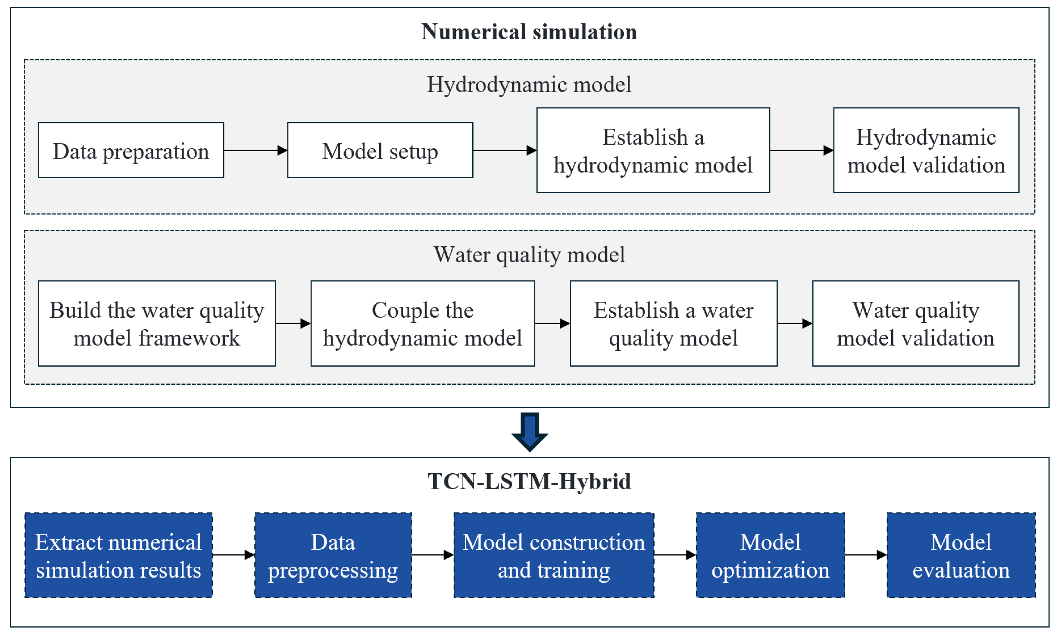
This study aims to predict the TN concentration in the Shenzhen Bay area by constructing a TCN-LSTM-Hybrid neural network model to achieve accurate predictions of the spatial distribution of TN concentrations. The overall technical framework is illustrated in Figure 1. First, a hydrodynamic model using Delft3D FM (Deltares, Delft, The Netherlands) is developed and validated to accurately simulate variations in water level and flow velocity. On this basis, a water quality model is constructed and coupled with the hydrodynamic model to simulate the transport and diffusion process of TN in the study area. Subsequently, TN concentration data are extracted from the numerical simulation results and combined with boundary inputs to build a comprehensive dataset (containing a total of 793,520 data samples). This dataset is divided into training, validation, and test sets in a 6:2:2 ratio to train the TCN-LSTM-Hybrid model. Through model optimization and evaluation, the predictive performance of the TCN-LSTM-Hybrid model is validated using multiple metrics, providing an efficient and reliable technical solution for the dynamic management of water quality in bay environments.

2.2. Study Area and Data Sources

This study focuses on the Shenzhen Bay area, located in the southern part of Shenzhen City, Guangdong Province, China, facing the Hong Kong Special Administrative Region across the sea. As shown in Figure 2, Shenzhen Bay covers a water area of approximately 60 square kilometers, with an average depth of around 3 m. It exhibits the typical characteristics of a shallow coastal bay, with a winding coastline and important ecological areas along its shore, such as the Futian Mangrove Nature Reserve and Shenzhen Bay Park. These areas serve as critical habitats for migratory birds. At the same time, Shenzhen Bay is also a key economic zone in Shenzhen, hosting several ports and industrial areas, including Shekou Port and Chiwan Port, playing a vital role in the city’s foreign trade and marine economy.

The hydrodynamic conditions of Shenzhen Bay are complex, influenced by multiple factors such as Pearl River runoff, tidal fluctuations, and monsoons. Water quality in the bay is of great concern, and the TN concentration, as a key water quality indicator, is affected by a combination of factors. Accurate prediction of TN concentration distribution is of great importance for water quality management and ecological protection in Shenzhen Bay. It contributes to early warnings of water quality changes and supports the formulation of scientific and effective pollution prevention strategies, ensuring the sustainable development of the bay’s ecological environment.

Meteorological data used in this study were obtained from the Shenzhen Meteorological Bureau’s automatic monitoring stations, the Hong Kong Observatory, and the King’s Park Meteorological Station in Hong Kong. Water quality data were provided by the Shenzhen Nearshore Waters Special Monitoring Report. The data collection period for both meteorological and water quality data spans from October 2021 to June 2022.

2.3. Physical Representation

The governing equations of the Delft3D hydrodynamic and water quality models are as follows:

(1)

Continuity equation

$${\displaystyle \frac{\partial \zeta }{\partial t}}+{\displaystyle \frac{1}{\sqrt{G_{\xi \xi }}\sqrt{G_{\eta \eta }}}}{\displaystyle \frac{\partial ((d+\zeta )u\sqrt{G_{\eta \eta }})}{\partial \xi }}+{\displaystyle \frac{1}{\sqrt{G_{\xi \xi }}\sqrt{G_{\eta \eta }}}}{\displaystyle \frac{\partial ((d+\zeta )v\sqrt{G_{\xi \xi }})}{\partial \eta }}=(d+\zeta )Q$$

(1)

where u = velocity in the ξ-direction;

v = velocity in the η-direction;

Q = flow variation per unit area caused by drainage or precipitation;

d = depth below the reference surface;

ζ = free surface elevation above the reference plane;

d + ζ = total water depth;

t = time.

(2)

Momentum equation

The momentum equation in the ξ direction is:

$$\begin{array}{l}{\displaystyle \frac{\partial u}{\partial t}}+{\displaystyle \frac{u}{\sqrt{G_{\xi \xi }}}}{\displaystyle \frac{\partial u}{\partial \xi }}+{\displaystyle \frac{v}{\sqrt{G_{\eta \eta }}}}{\displaystyle \frac{\partial u}{\partial \eta }}+{\displaystyle \frac{\omega }{d+\zeta }}{\displaystyle \frac{\partial u}{\partial \sigma }}-{\displaystyle \frac{v^2}{\sqrt{G_{\xi \xi }}\sqrt{G_{\eta \eta }}}}{\displaystyle \frac{\partial \sqrt{G_{\eta \eta }}}{\partial \xi }}+{\displaystyle \frac{uv}{\sqrt{G_{\xi \xi }}\sqrt{G_{\eta \eta }}}}{\displaystyle \frac{\partial \sqrt{G_{\xi \xi }}}{\partial \eta }}\\ -fv=-{\displaystyle \frac{1}{{\rho }_0\sqrt{G_{\xi \xi }}}}{P}_{\xi }+F_{\xi }+{\displaystyle \frac{1}{{(d+\zeta )}^2}}{\displaystyle \frac{\partial }{\partial \sigma }}({\upsilon }_v{\displaystyle \frac{\partial u}{\partial \sigma }})+M_{\xi }\end{array}$$

(2)

The momentum equation in the η direction is:

$$\begin{array}{l}{\displaystyle \frac{\partial v}{\partial t}}+{\displaystyle \frac{u}{\sqrt{G_{\xi \xi }}}}{\displaystyle \frac{\partial v}{\partial \xi }}+{\displaystyle \frac{v}{\sqrt{G_{\eta \eta }}}}{\displaystyle \frac{\partial v}{\partial \eta }}+{\displaystyle \frac{\omega }{d+\zeta }}{\displaystyle \frac{\partial v}{\partial \sigma }}-{\displaystyle \frac{u^2}{\sqrt{G_{\xi \xi }}\sqrt{G_{\eta \eta }}}}{\displaystyle \frac{\partial \sqrt{G_{\xi \xi }}}{\partial \eta }}+{\displaystyle \frac{uv}{\sqrt{G_{\xi \xi }}\sqrt{G_{\eta \eta }}}}{\displaystyle \frac{\partial \sqrt{G_{\eta \eta }}}{\partial \xi }}\\ -fu=-{\displaystyle \frac{1}{{\rho }_0\sqrt{G_{\eta \eta }}}}{P}_{\eta }+F_{\eta }+{\displaystyle \frac{1}{{(d+\zeta )}^2}}{\displaystyle \frac{\partial }{\partial \sigma }}({\upsilon }_v{\displaystyle \frac{\partial v}{\partial \sigma }})+M_{\eta }\end{array}$$

(3)

where w = flow velocity in the vertical direction;

σ = proportional vertical coordinate;

ρ₀ = density of water;

P_ξ = hydrostatic pressure gradient in the ξ-direction;

P_η = hydrostatic pressure gradient in the η-direction;

F_ξ = effects of horizontal Reynolds stresses causing imbalance in the ξ-direction;

F_η = effects of horizontal Reynolds stresses causing imbalance in the η-direction;

M_ξ = effects of external factors on momentum in the ξ-direction;

M_η = effects of external factors on momentum in the η-direction;

${\upsilon }_v$ = vertical eddy viscosity coefficient.

(3)

Convection-diffusion-reaction equation

$${\displaystyle \frac{\partial C}{\partial t}}+v_x{\displaystyle \frac{\partial C}{\partial x}}-D_x{\displaystyle \frac{{\partial }^{2}C}{\partial x^2}}+v_y{\displaystyle \frac{\partial C}{\partial y}}-D_y{\displaystyle \frac{{\partial }^{2}C}{\partial y^2}}+v_z{\displaystyle \frac{\partial C}{\partial z}}-D_z{\displaystyle \frac{{\partial }^{2}C}{\partial z^2}}=S+f_R(C,t)$$

(4)

where C = concentration;

D_x = diffusion coefficient in the x-direction;

D_y = diffusion coefficient in the y-direction;

D_z = diffusion coefficient in the z-direction;

S = inflow term;

f_R = reaction term.

The Delft3D-WAQ model simulates changes in total nitrogen concentration through a series of ecological processes, among which nitrification is one:

$${\mathrm{NH}}_4^{+}+2O_2\to {\mathrm{NO}}_3^{-}+2H^{+}+H_{2}O$$

(5)

Denitrification:

$$4{\mathrm{NO}}_3^{-}+5{\mathrm{CH}}_{2}O+4H^{+}\to 2N_2+5{\mathrm{CO}}_2+11H_{2}O$$

(6)

2.4. Numerical Experiments

The latitude of the numerical model used in this study is set to 22.48°, with 10 vertical layers. The simulation period spans from 1 October 2021 to 30 June 2022, using a time step of 30 s. The gravitational acceleration is set to 9.81 m/s², water density to 1000 kg/m³, and air density to 1.205 kg/m³. The wind drag coefficient is 0.00063 for wind speeds between 0 and 100 m/s, and 0.00723 for speeds above 100 m/s. The Manning roughness coefficient is 0.023. Horizontal and vertical eddy viscosity and diffusion coefficients are set to 1 m²/s and 5 × 10⁻⁵ m²/s, respectively, to simulate turbulent mixing at different scales within the water body. The model employs the k-ε turbulence model. The Secchi depth is set to 2 m, and both the Stanton and Dalton numbers are set to −1. In terms of spatial discretization, a structured grid is used, with an average grid cell length of approximately 150 m. Orthogonality tests show that the cosine of the angle between grid lines is less than 0.02 at all grid nodes, meeting the spatial accuracy requirements of the numerical model.

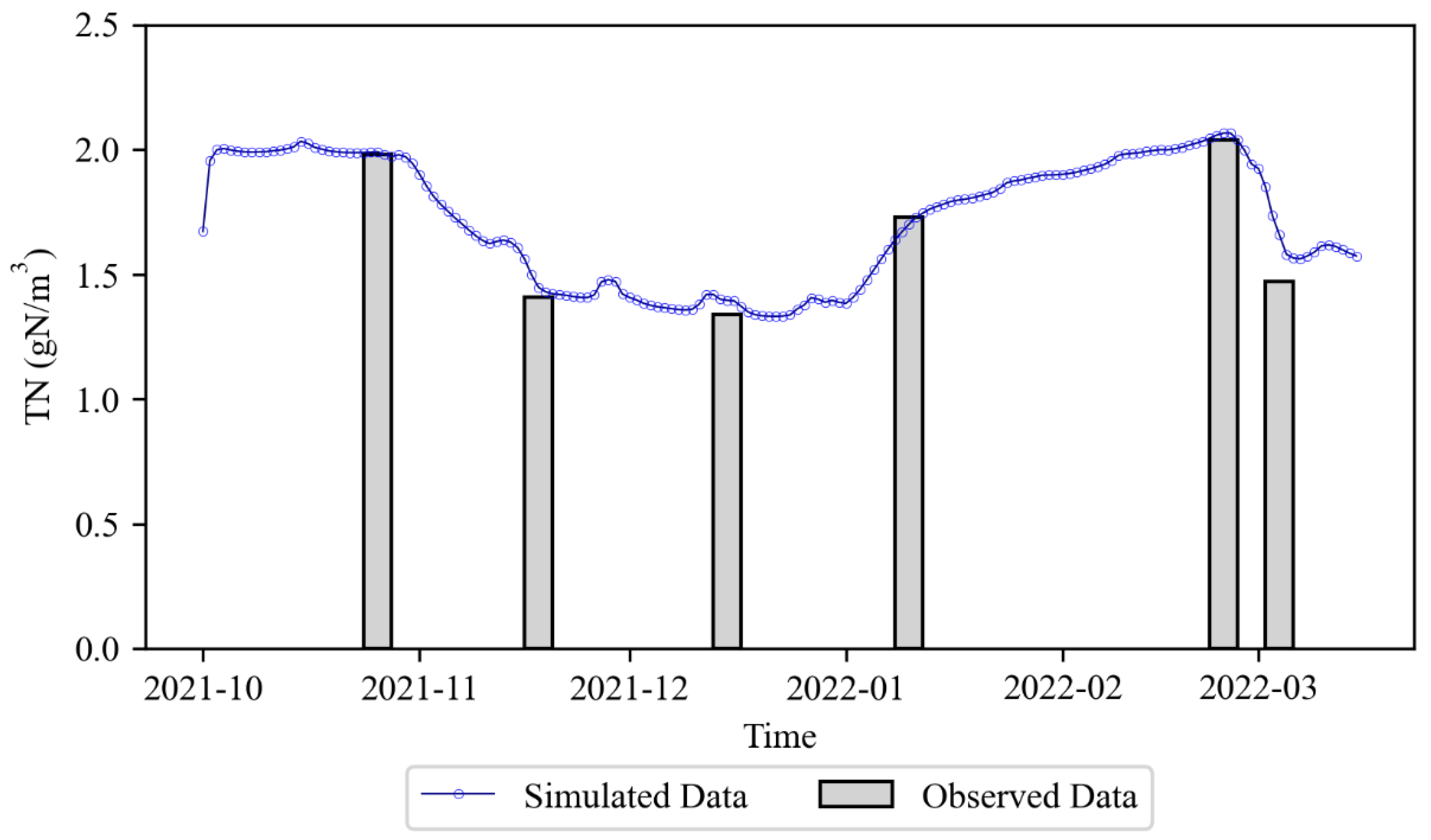
The water quality model is based on the outputs of the hydrodynamic model and simulates the spatiotemporal variation in total nitrogen by coupling the hydrodynamic field with water quality processes. During the coupling process, mass conservation was strictly verified to ensure that the input, output, and transformation of total nitrogen comply with physical and chemical principles. The initial conditions of the water quality model were obtained through spatial interpolation of observed total nitrogen concentrations from various monitoring points. Boundary conditions were established based on the “Shenzhen Coastal Waters Special Monitoring Point Information Table”, selecting the monitoring site LH016 (longitude 113.8925, latitude 22.4378) located at the bay boundary as the water quality boundary input point. Observational data of total nitrogen concentration at this site were used to drive the model boundary, ensuring that the model accurately reflects the impact of external nutrient inputs on the water quality within the study area.

2.5. TCN-LSTM-Hybrid Model

This study developed a hybrid deep learning model that integrates a Temporal Convolutional Network (TCN) with a Long Short-Term Memory (LSTM) network, referred to as the TCN-LSTM-Hybrid model. The model takes as input the total nitrogen concentrations at four key boundary points over the past six days and outputs the predicted total nitrogen concentration distribution in the Shenzhen Bay area for the next day. It is worth noting that the numerical model built with Delft3D has coupled and solved the hydrodynamic processes within the study area (including tidal forcing, flow fields, mixing, and diffusion) together with external boundary forcing. As a result, the internal TN field already reflects the combined effects of hydrodynamics and boundary pollutant inputs. In this context, the role of the deep learning model is to learn the empirical mapping of “how boundary TN drives the internal TN spatial distribution under given hydrodynamic conditions.” As shown in Figure 3, the architecture of the TCN-LSTM-Hybrid model begins with a TCN layer as the feature extraction module. This layer uses multiple dilated convolution layers to extract features from the input time-series data. The dilation factors are set to [1,2,4,8], the convolution kernel size is 5, and the number of convolutional channels is 512, allowing the model to capture multi-scale temporal dependencies. The output of the TCN layer retains the temporal structure and serves as the input for the subsequent LSTM layer, which is configured with 256 neurons to further enhance the model’s understanding of sequential patterns. A Dropout layer is then added to prevent overfitting, followed by a fully connected layer to generate the final prediction. The output layer uses the LeakyReLU activation function to avoid gradient vanishing problems caused by ReLU saturation, thereby improving the model’s nonlinear fitting capability. During model training, both input and output variables were normalized to the [0, 1] range, and the predictions were subsequently denormalized to recover the original physical quantities. The data sources, validated through the Delft3D numerical model and monitoring, showed no anomalies. The model was compiled using the Adam optimizer and the mean squared error (MSE) loss function, with a dynamically adjusted learning rate. Training was performed for 800 epochs using the training dataset, while performance was monitored on the validation set to prevent overfitting. This model architecture effectively combines the strengths of TCN and LSTM, providing strong support for the accurate prediction of total nitrogen concentration distributions.

2.6. Reference Methods

To further explore the applicability and performance of different deep learning architectures in water quality time-series prediction, this study separately constructed and tested TCN, LSTM, GRU, and MLP models in addition to the TCN-LSTM-Hybrid model. These models served as comparative baselines to further validate the effectiveness and advantages of the TCN-LSTM-Hybrid model in predicting total nitrogen concentrations in the Shenzhen Bay area. To ensure that different models were evaluated under comparable conditions, all comparison models were uniformly configured with the LeakyReLU activation function and the Adam optimizer, trained for 800 epochs, and monitored on the validation set for performance changes.

2.6.1. TCN Model

The TCN model is an improved causal convolutional neural network capable of effectively capturing long-term temporal dependencies through dilated convolutions, achieving a good balance between modeling efficiency and accuracy. In this study, the TCN layer was configured with 64 convolutional filters and a kernel size of 3, using a multi-layer dilated convolution structure with dilation rates of [1, 2, 4, 8] to expand the receptive field and model long-term dependencies. The ‘return_sequences’ parameter was set to ‘False’ so that the layer outputs a unified temporal feature representation. A Dropout layer with a dropout rate of 0.5 was subsequently added to alleviate overfitting. A fully connected layer was then connected to output the total nitrogen concentration field of the Shenzhen Bay area, and a LeakyReLU activation function was applied to introduce nonlinearity and enhance the model’s expressive power.

2.6.2. LSTM Model

The LSTM network is a type of recurrent neural network capable of capturing long-term dependencies, making it particularly suitable for handling nonlinear and highly time-varying time series data. In this study, a predictive model with a two-layer LSTM structure was constructed. The first LSTM layer was configured with 200 neurons, using the tanh activation function and setting ‘return_sequences = True’ to pass the temporal features to the subsequent LSTM layer. To enhance the model’s generalization ability, a Dropout layer with a dropout rate of 0.8 was added after the first layer to mitigate the risk of overfitting. The second LSTM layer contained 150 neurons with ‘return_sequences = False’, outputting the final temporal feature vector, followed by another Dropout layer. The output layer was a fully connected layer, with the number of nodes matching the target prediction dimensions, and it used the LeakyReLU activation function to avoid the gradient vanishing problem associated with traditional ReLU.

2.6.3. GRU Model

Gated Recurrent Unit (GRU) is a lightweight variant of recurrent neural networks (RNN) that effectively addresses the vanishing gradient problem of traditional RNNs by introducing update and reset gates. In this study, the GRU model is constructed with two GRU layers. The first layer contains 200 neurons, uses the tanh activation function, and sets ‘return_sequences = True’ to retain the full time series output for processing by the next layer. A Dropout layer with a dropout rate of 0.8 is added to mitigate overfitting. The second GRU layer has 150 units and sets ‘return_sequences = False’ to compress its output into the final temporal feature representation, also followed by a Dropout layer to further improve generalization. At the output end, the model includes a fully connected layer with the number of nodes matching the target prediction dimensions, using the LeakyReLU activation function. During model compilation, the Adam optimizer is employed, and MSE is used as the loss function to suit the regression nature of total nitrogen concentration prediction in this study.

2.6.4. MLP Model

Multilayer Perceptron (MLP) is a typical feedforward neural network structure that models complex relationships between input features and output variables through layer-by-layer nonlinear mappings. In this study, the MLP model consists of four fully connected layers. The input layer accepts flattened sequence features, followed by a first fully connected layer with 256 neurons, and two subsequent hidden layers with 128 and 64 neurons, respectively. Each layer uses the LeakyReLU activation function to enhance the model’s nonlinear representation capability, and Dropout layers with rates of 0.5, 0.5, and 0.3 are applied after each layer to alleviate overfitting and improve model generalization. The output layer has a number of neurons matching the target variable, used to predict the spatial distribution of total nitrogen concentration in the Shenzhen Bay area for the next day.

3. Results

3.1. Numerical Results

Figure 4 shows the comparison between the simulated TN concentration results from the numerical model constructed in this study and the measured data. The simulated data aligns well with the measured data in overall trend, accurately predicting both high and low TN concentrations at multiple key points. Between two measured time points, the simulation exhibits smooth and realistic fluctuations, reflecting the model’s ability to fit continuous variation processes and its strong capability to capture the evolving pattern of total nitrogen concentration distribution. Although slight deviations occur at some time points (e.g., March 2022), the overall simulation errors are small, with error fluctuations within an acceptable range and no systematic bias toward overestimation or underestimation. Additionally, the calculated RMSE is 0.083 gN/m³ and MAE is 0.058 gN/m³, indicating small errors. These results further validate the accuracy and stability of the numerical model in predicting TN concentration, providing reliable support for subsequent machine learning training.

Spatial distribution maps were generated using numerical simulation results randomly selected from 16 days, as shown in Figure 5. In October and November 2021, total nitrogen concentrations were relatively low, possibly due to lower water temperatures suppressing microbial activity, thereby slowing down nitrogen transformation and accumulation rates. By January and February 2022, concentrations increased significantly, especially from 24 February to 10 March 2022, when concentrations at some river inflow points to the bay were notably higher than in other areas, reaching nearly 3.08 gN/m³. Overall, concentrations gradually increased from the bay mouth toward the bay head, with the concentration gradient rising from outside to inside. The numerical simulation results effectively reflect the spatiotemporal variation pattern of total nitrogen concentration, further validating the reliability of the numerical model. These simulation results can subsequently be used as ground truth to train machine learning models.

3.2. Performance of the TCN-LSTM-Hybrid Model

To evaluate the spatial prediction capability of the constructed TCN-LSTM-Hybrid Model for TN concentration simulation, simulation results from four randomly selected days were compared with the ground truth, as shown in Figure 6. The TCN-LSTM-Hybrid model’s simulated spatial distribution of TN concentration at different time points is generally consistent with the ground truth, effectively capturing the spatial variation characteristics of total nitrogen concentration in the Shenzhen Bay area. The model’s simulation results closely match the ground truth in terms of concentration gradients and overall trends, particularly showing a high degree of fit in the concentration differences and locations of high-value regions between the bay mouth and bay head. Although minor deviations exist in some areas, the overall simulation results align well with the ground truth, indicating that the TCN-LSTM-Hybrid model demonstrates high accuracy and generalization ability in simulating the spatial distribution of total nitrogen concentration.

To evaluate the temporal prediction capability of the TCN-LSTM-Hybrid Model, six random points were selected to generate time series line charts comparing the model outputs with the Ground Truth, as shown in Figure 7. The results indicate that the TCN-LSTM-Hybrid Model demonstrates good fitting performance at different locations, effectively capturing the variation trends and oscillation characteristics of TN concentration. The differences between the model simulations and the Ground Truth are minimal, with high accuracy in predicting both peaks and troughs, indicating that the model not only captures overall trends but also possesses strong local responsiveness. The R² values at all monitoring points exceed 0.96, reaching up to 0.988, showing a high correlation between the predictions and Ground Truth; meanwhile, RMSE values range between 0.023 and 0.042 gN/m³, keeping errors at a low level. Overall, the TCN-LSTM-Hybrid Model exhibits strong robustness and generalization ability in simulating the spatiotemporal variations in total nitrogen, capable of adapting to the complex water quality dynamics in the Shenzhen Bay area.

3.3. Performance of the Reference Methods

In this study, a comparative analysis was conducted on the predictive performance of four reference algorithms (LSTM, GRU, MLP, and TCN) across the training, validation, and testing datasets, as shown in Figure 8, Figure 9, Figure 10 and Figure 11. The LSTM model achieved R² values above 0.88 and RMSE values below 0.061 gN/m³ across all three datasets, with the predicted values aligning closely with the Ground Truth along the diagonal, indicating good fitting performance and generalization ability. The GRU model’s predicted point clouds were mostly concentrated near the ideal fitting line, with no significant systematic bias. The MLP model performed well on the training and testing sets and slightly less so on the validation set, while still maintaining high prediction accuracy. The TCN model showed R² values close to 0.90 on all datasets, with RMSE ranging from 0.054 to 0.066 gN/m³. Its predictions were evenly distributed near the 1:1 isometric line, demonstrating model stability. Overall, all four algorithms exhibited good predictive capabilities and were able to effectively capture the distribution characteristics of total nitrogen concentration. Further comparative analysis with the TCN-LSTM-Hybrid Model will be presented in the Section 4.

4. Discussion

This study introduces, for the first time, a machine learning approach to model and predict the spatiotemporal distribution characteristics of TN concentration in the Shenzhen Bay area. By constructing a TCN-LSTM-Hybrid Model that leverages the strengths of temporal sequence modeling, the study achieves efficient prediction of TN concentration across the study area. In this study, the target values were predicted using the features from the previous six days rather than through a simple time series prediction. During the feature construction stage, each sample’s features were derived from the data of the past six days, which inherently contained temporal information. Therefore, even when random splitting was applied during the data partitioning stage, it did not result in any information from future data leaking into the training set. The model combines the parallel computing advantages of TCN in processing long sequences with the strong nonlinear sequence modeling capabilities of LSTM networks. This combination addresses the limitation of traditional TCN models in responding to complex dynamic changes. It enables more comprehensive capture of the temporal and spatial variation patterns of total nitrogen concentration, thereby enhancing the model’s adaptability and generalization ability in dynamic aquatic environments. This research provides a novel technical route for water quality forecasting in complex bay environments like Shenzhen Bay and offers a valuable reference for similar studies in other regions, demonstrating the immense potential of machine learning in environmental science.

In this study, machine learning methods overcome the limitations of traditional experimental measurements and CFD simulations. While experimental measurements offer high precision, they demand substantial human, material, and time resources, making large-scale and long-term continuous monitoring difficult. CFD approaches can handle complex physical processes but involve complicated modeling procedures, high computational costs, and inherent uncertainty in the results. Given the complex hydrodynamics and pollutant transport processes in Shenzhen Bay, machine learning can autonomously learn complex patterns and relationships from data and provide rapid predictions for new data within a short time. Under the same computer configuration (13th Gen Intel(R) Core(TM) i5 processor and 16 GB of RAM), the proposed machine learning model in this study can complete predictions within a few minutes, whereas conventional CFD simulations require several hours to obtain results. This greatly reduces time and cost, enabling more efficient acquisition of dynamic TN concentration distribution in Shenzhen Bay and significantly enhancing the efficiency and practicality of the research.

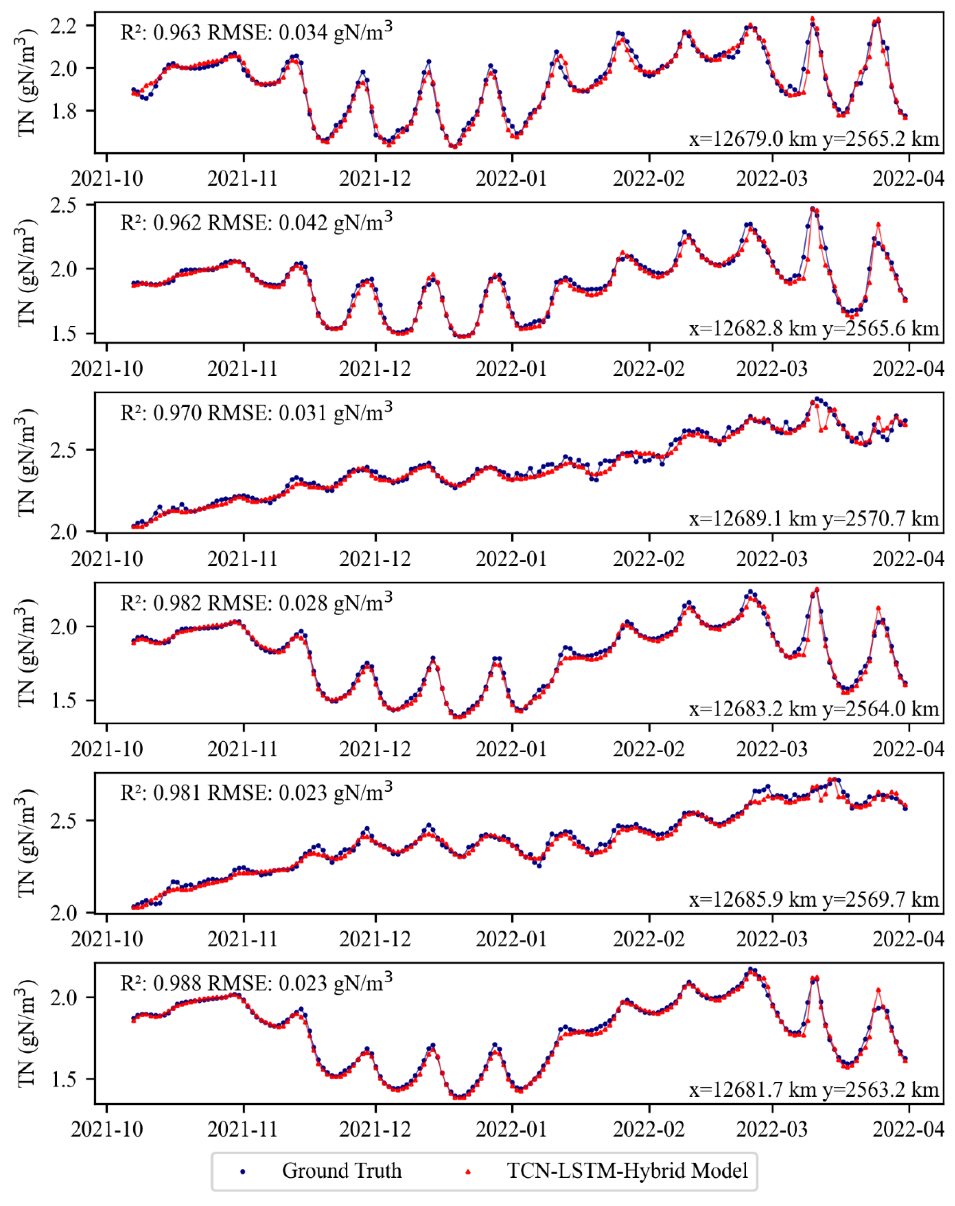
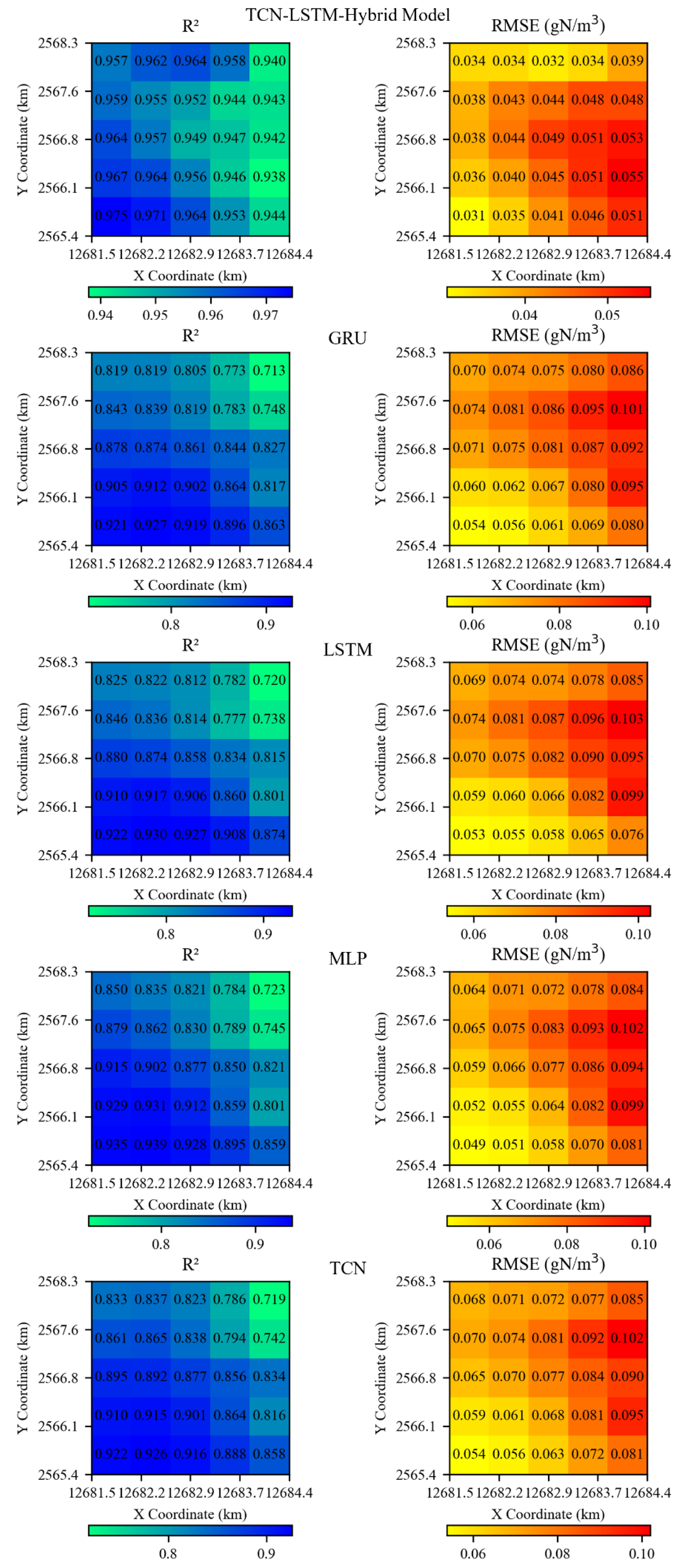
Further comparison between the TCN-LSTM-Hybrid Model and other machine learning models was conducted by randomly selecting 25 coordinate points within local regions of Shenzhen Bay, calculating the R² and RMSE values for each point, as shown in Figure 12. The performance differences among various machine learning models in predicting TN concentration are evident. The TCN-LSTM-Hybrid Model maintains high R² values (0.940–0.975) and the lowest RMSE values, with a minimum of 0.031 gN/m³ across most spatial locations, significantly outperforming GRU, LSTM, TCN, and MLP models. In contrast, GRU, LSTM, TCN, and MLP show certain predictive capabilities in some areas, but most coordinate points exhibit R² values below 0.9 and RMSE values generally exceeding 0.06 gN/m³, especially with higher fluctuation in accuracy near boundary regions. 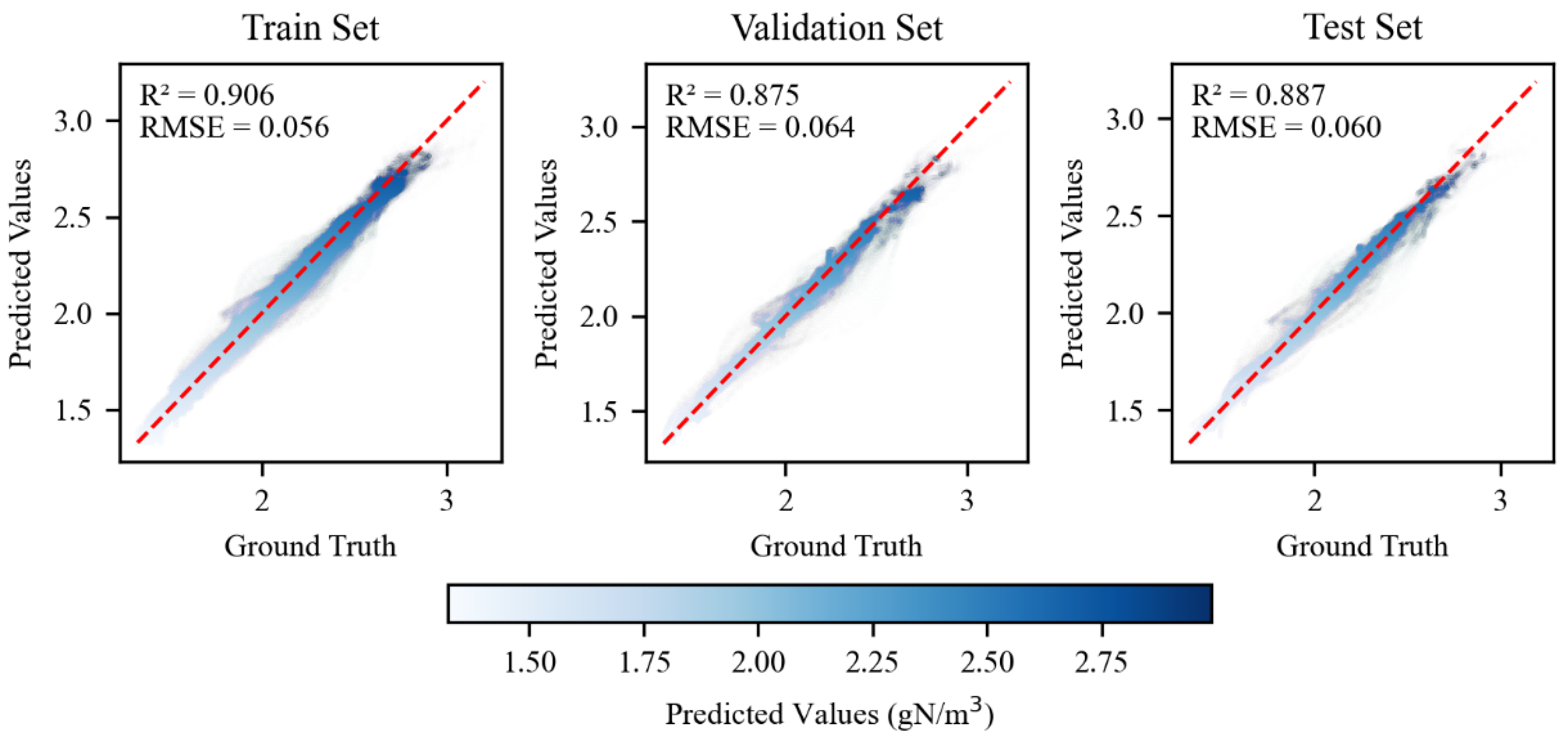To further verify the statistical significance of model differences, paired t-tests were conducted between the TCN-LSTM-Hybrid Model and each reference algorithm on the training, validation, and test sets, with the results shown in

Table 1. Paired t-test results of model errors.

Comparison	Train Set			Validation Set			Test Set
	Mean Diff	t-Statistic	p_Value	Mean Diff	t-Statistic	p_Value	Mean Diff	t-Statistic	p_Value
TCN-LSTM-Hybrid vs. GRU	−0.0025	−307.38	p < 0.001	−0.0021	−126.88	p < 0.001	−0.0023	−157.29	p < 0.001
TCN-LSTM-Hybrid vs. LSTM	−0.0026	−280.09	p < 0.001	−0.0017	−100.98	p < 0.001	−0.0022	−140.12	p < 0.001
TCN-LSTM-Hybrid vs. TCN	−0.0024	−327.26	p < 0.001	−0.0023	−134.94	p < 0.001	−0.0022	−152.93	p < 0.001
TCN-LSTM-Hybrid vs. MLP	−0.0020	−290.90	p < 0.001	−0.0020	−117.99	p < 0.001	−0.0019	−144.75	p < 0.001

. The errors of the TCN-LSTM-Hybrid Model were significantly lower than those of the GRU, LSTM, TCN, and MLP models across all datasets, with highly significant statistical results. These findings further confirm the strong robustness and generalization ability of the TCN-LSTM-Hybrid Model. Its performance surpasses that of using LSTM or TCN alone, indicating that the multi-scale temporal feature extraction capability of TCN and the long-sequence memory capability of LSTM complement each other through their synergy, thereby enhancing the model’s adaptability and generalization to the complex hydrodynamic processes in Shenzhen Bay.

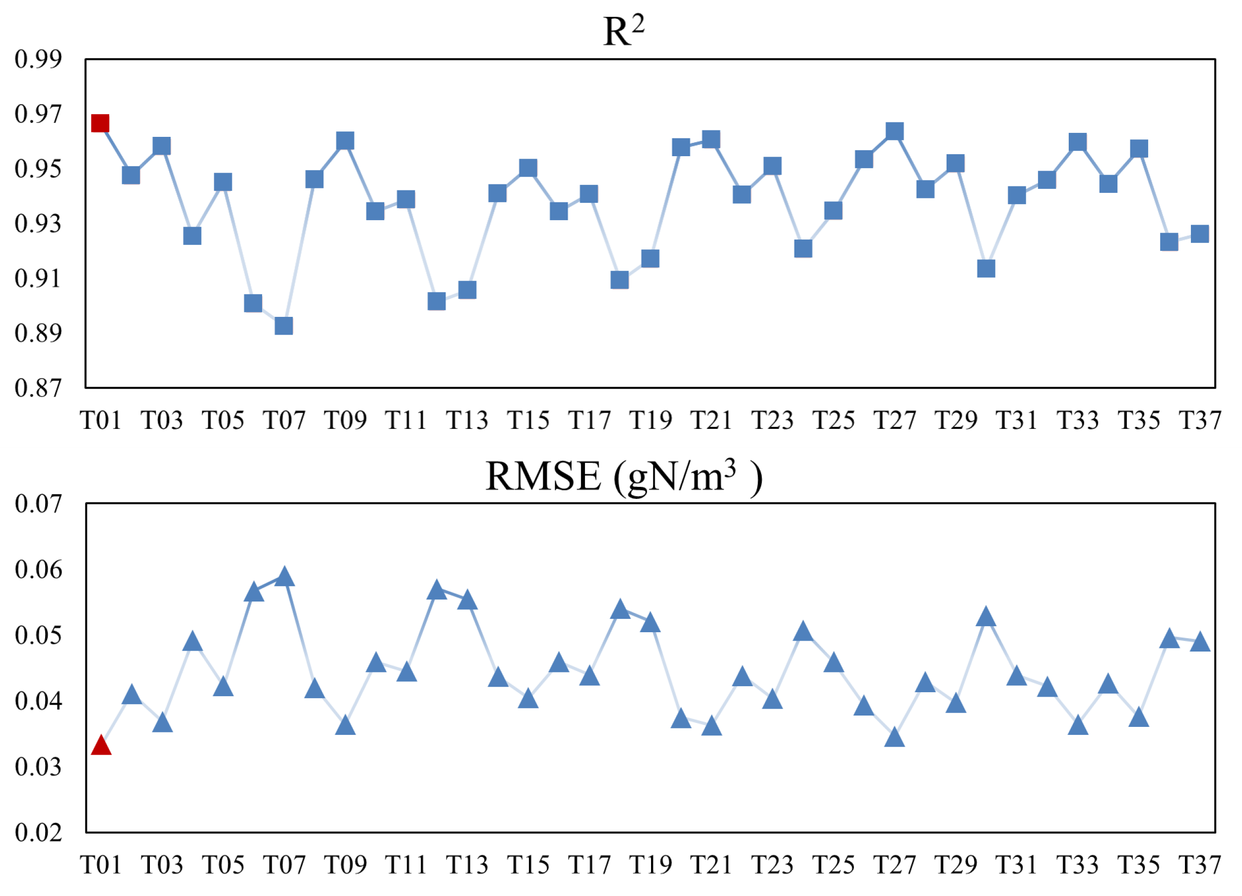
To further verify the stability and robustness of the TCN-LSTM-Hybrid Model under different structural configurations, a hyperparameter sensitivity analysis was conducted, as shown in Figure 13. In the figure, T01 represents the TCN-LSTM-Hybrid Model, while T02 to T37 correspond to 36 hyperparameter combinations designed by varying the number of convolutional filters (64, 128), kernel sizes (2, 3, 5), dropout ratios (0.1, 0.3, 0.5), and the number of LSTM units (64, 128). For each combination, the R² and RMSE values on the test set were calculated. The results demonstrate that the model achieves consistently strong performance, with all R² values exceeding 0.89 and RMSE controlled within 0.06, indicating the inherent reliability of the framework. Notably, the TCN-LSTM-Hybrid Model exhibits significantly higher predictive accuracy compared with other configurations, further validating the reliability and robustness of the proposed approach. Meanwhile, Monte Carlo Dropout was employed to perform uncertainty analysis, where multiple forward passes with injected randomness were used to generate predictive distributions. As shown in Figure 14, the predicted mean curve closely follows the variation trend of the observed values, and the 95% confidence interval largely encompasses the true values, indicating that the model not only delivers strong predictive performance but also provides a reliable assessment of its own predictive uncertainty.

TN is one of the most critical and representative pollution indicators in the Shenzhen Bay area. As an exploratory study, this work selects TN as the entry point to verify the effectiveness and feasibility of the proposed modeling approach. This study primarily focuses on predicting the distribution of TN concentrations and has not yet fully considered the synergistic relationships with other water quality parameters. The water quality in the Shenzhen Bay area is influenced by multiple factors, such as total phosphorus, chlorophyll, etc. Future research can expand the scope of the model by incorporating a broader range of water quality parameters to develop a multi-parameter, multi-dimensional integrated prediction model. This would provide a more comprehensive representation of the water quality status and its evolving trends in the Shenzhen Bay area, offering more scientific and effective support for decision making by relevant authorities. The numerical simulations and training data used in this study did not cover a complete seasonal cycle or multi-year variations, which may limit the model’s extrapolation ability under cross-seasonal or interannual extreme hydrodynamic conditions. Future research could extend the temporal span to include more years and full seasonal cycles, thereby enhancing the model’s generalization capability under different seasonal conditions. It should be noted that, ideally, measured datasets should be used to train machine learning models to ensure a high degree of consistency between predictions and real-world conditions. However, due to the practical challenges of conducting long-term and large-scale water quality monitoring in semi-enclosed bay areas, this study employed validated numerical model outputs as the “ground truth” for model training. Although this approach can, to some extent, ensure the reliability of the predictions, it is still subject to limitations arising from potential discrepancies with in situ observations. In the future, if more comprehensive and continuous observational datasets become available, they could be used to train and validate the model, thereby further enhancing its robustness and applicability. This study primarily focuses on predicting TN concentrations under typical hydrodynamic conditions in Shenzhen Bay. Due to limitations in data availability, extreme events such as storms or abnormal wastewater discharges were not included. Future work will aim to extend the model to incorporate these extreme scenarios, thereby further evaluating the stability and reliability of the predictions. More importantly, the deep learning framework proposed in this study has the potential to be integrated with real-time coastal zone management systems in the future. By incorporating real-time monitoring sensor networks and data assimilation techniques, it can achieve online prediction and dynamic early warning of total nitrogen and other pollutants. The research outcomes can be directly applied to the integrated management practices of Shenzhen Bay and similar bays, thereby significantly enhancing their practical value.

5. Conclusions

This study focuses on the critical issue of predicting TN concentration distribution in the Shenzhen Bay area. To address the limitations of existing methods in simulating and forecasting TN distribution, a TCN-LSTM-Hybrid Model was developed to enable efficient prediction of TN concentration across the region. The results demonstrate that the model effectively leverages the strengths of TCN and LSTM networks to handle complex time-series data, achieving high-accuracy predictions of TN distribution. The model performs well across training, validation, and test datasets, showing strong generalization capabilities and significantly outperforming traditional models such as GRU, LSTM, MLP, and TCN. These findings validate the feasibility and applicability of the TCN-LSTM-Hybrid Model in marine water quality modeling and provide a novel approach for high-precision water quality prediction in complex marine environments. In the future, more water quality parameters can be incorporated to build a multi-parameter, multi-dimensional integrated prediction model, offering stronger support for water quality protection and ecological sustainability.