Abstract
Predictive maintenance of semi-autogenous grinding (SAG) mills reduces unplanned downtime and improves throughput. This study develops a data-driven prognostic model for production SAG mill using four years of operational data (temperature, voltage, current, motor speed, etc.). We follow a MATLAB (R2025a)-based prognostics and health management (PHM) workflow: data cleaning and synchronization; feature engineering in time and frequency domains (statistical moments, spectral power, bandwidth); normalization and clustering to separate operating regimes; and labeling of run-to-failure sequences for a recurring electrical failure mode. A health indicator is derived by scoring candidate features for monotonicity, trendability, and prognosability and fusing them into a condition index. Using MATLAB Predictive Maintenance Toolbox, we train and validate multiple Remaining Useful Life (RUL) learners including similarity-based, regression, and survival models on run-to-failure histories, selecting the best via cross-validated error and prediction stability. On held-out sets, the selected model forecasts RUL consistent with observed failure dates, providing actionable lead time for maintenance planning. The results highlight the practicality of deploying a PHM pipeline for SAG mills using existing plant data and commercial toolchains.
1. Introduction
Industrial maintenance generally follows three strategies: reactive maintenance (run to failure), preventive maintenance (time- or usage-based), and predictive maintenance (condition-based, driven by monitoring and analytics). Authoritative reviews describe the shift from corrective and preventive approaches toward predictive maintenance as sensors, data infrastructure, and analytics mature [1]. In mining, field studies that map current practices in East Canadian operations report strong expectations for explainable, data-driven tools and a gradual transition from preventive to predictive strategies to improve planning and reduce unplanned stoppages [2]. Recent reviews and implementations in mining show that machine learning models trained on multi-sensor data, combined with robust data preparation and labeling, consistently improve early fault detection and Remaining Useful Life estimation compared with fixed-interval servicing [3]. Dayo-Olupona et al. survey predictive maintenance practices across mining equipment and report that classification, anomaly detection, and RUL methods become reliable once data infrastructure and run-to-failure histories are available, which strengthens the business case for predictive strategies [4]. Digital twin frameworks tailored to mining integrate real-time measurements with physics-based or data-driven models to support condition monitoring, what-if maintenance scheduling, and production optimization; Nobahar et al. classify mining twins across the value chain and highlight sensing, data fusion, and AI as core enablers for condition-based maintenance [5]. A complementary system view shows that an Industrial Internet of Things platform provides the sensing and connectivity backbone for predictive maintenance analytics in operating mines; Miñón et al. describe and validate a multi-level IIoT stack deployed in European mining use cases that standardizes data capture and feeds predictive applications [6]. For comminution circuits specifically, data-driven models for Semi-Autogenous Grinding (SAG) mills can forecast critical states such as overloads and can predict liner wear, which enables timely interventions and helps avoid costly shutdowns [7,8,9,10]. Taken together, these developments indicate that, compared with run-to-failure or fixed-interval servicing, condition-based predictive maintenance is the most effective strategy for minimizing unexpected downtime and stabilizing throughput in mineral processing plants.
Machine learning (ML) has accelerated predictive maintenance (PdM) across mining by turning multi-year sensor streams (vibration, current, temperature, and process images) into early-warning indicators that cut unplanned downtime. In mineral processing, a comprehensive review showed ML’s three core roles, data-based modeling, fault detection/diagnosis, and machine vision, are now standard for monitoring complex circuits and anticipating failures, laying the groundwork for health indicators and RUL workflows in plants [11]. Deep learning has also proven effective for plant-level anomaly detection: for example, convolutional network features combined with a support vector classifier accurately flag flotation faults in production imagery, enabling real-time alerts before quality losses propagate downstream [12].
In industrial practice, the PdM algorithm is built as an iterative pipeline: acquire representative data, preprocess it, derive condition indicators (features), train and validate models for anomaly detection/diagnosis/RUL, and finally deploy the model to the plant or edge device. This end-to-end process is widely described in the engineering literature and aligns with the workflow popularized by MathWorks for PdM development [13]. The data step is foundational. PdM uses both measured sensor data, including vibration, acoustic emissions, motor currents, temperatures, flows, densities, and particle-size proxies, and generated data from simulations when real failures are rare or risky to capture. Physics-based models or digital twins are often used to synthesize faulty operating regimes to augment training sets and to support what-if analysis during operations [14,15,16]. In mineral-processing circuits, especially SAG mills, relevant signals typically include mill power and torque, rotational speed, load or pebble recycle, lube-oil pressures or temperatures, trunnion bearing temperatures, hydrocyclone feed or pressure, and downstream quality variables. These signals are affected by ore hardness variability, feed size distribution, liners/lifters wear, and control actions, making PdM particularly valuable for reducing unplanned stoppages and stabilizing throughput.
After data acquisition, preprocessing standardizes the raw streams by some processes including time alignment, resampling, filtering, outlier handling, operating-state segmentation, and data quality tagging. Feature engineering then converts raw signals into condition indicators with discriminative power, statistics in time, frequency or time–frequency domains, envelope or cepstral features for bearings meshes, harmonics and sidebands from gearless mill drives (GMDs), and health indices derived from multivariate projections. The model-building stage typically addresses one of three goals: anomaly detection, fault identification, and RUL estimation (prognostics) [17], where survival or degradation models forecast time-to-maintain within confidence bounds.
For deployment on a large scale, predictive maintenance models must be properly packaged and integrated with the plant’s operational and maintenance systems, such as supervisory control and data acquisition (SCADA) platforms or computerized maintenance management systems (CMMSs). In some cases, they also need to be installed directly on local hardware close to the equipment to ensure a fast response and reliable operation. The business benefits of predictive maintenance such as reducing downtime, controlling maintenance costs, and planning spare parts are achieved only when models are successfully deployed in real operations, not merely when they show accuracy in offline testing [18,19]. This practical workflow aligns closely with the functional blocks defined in ISO 13374 for condition monitoring and diagnostics: Data Acquisition (DA), Data Manipulation (DM), State Detection (SD), Health Assessment (HA), Prognostics (PR), and Advisory Generation (AG), as well as the corresponding requirements for communication and presentation. Employing these standards as an architectural framework ensures that a predictive maintenance solution for a grinding circuit remains modular, interoperable, and auditable, from the initial sensor layer through prognostics and ultimately to the generation of work-order recommendations [20,21].
In this study, we operationalize the workflow with MATLAB because its toolboxes cover the full PdM stack end-to-end. Predictive Maintenance Toolbox provides apps and functions to manage ensembles, engineer and rank condition indicators, detect anomalies, and estimate RUL using similarity-based, survival, and degradation models methods that map directly onto industrial prognostics practice and recent reviews of PdM in mining and manufacturing. For feature design on SAG-mill signals (vibration, current, acoustic), Signal Processing Toolbox offers robust time–frequency analysis (spectrogram/STFT, reassignment, synchro squeezing) and related feature extractors suitable for nonstationary machinery data. Model training and validation leverage Statistics and Machine Learning Toolbox covering classification and regression algorithms with cross-validation and Bayesian hyperparameter optimization so that fault detectors or health indices can be tuned systematically. Finally, MATLAB streamlines deployment of trained PdM models to plant systems and edge targets, enabling real-time scoring alongside historians/SCADA and aligning with production requirements highlighted in the PdM implementation literature.
This paper is organized as follows: Section 2 describes SAG-mill data acquisition, including temperature, pressure, current, voltage, and speed of plants. Section 3 details preprocessing and feature extraction to construct the modeling dataset, culminating in a consolidated training table that explicitly includes run-to-failure sequences. Section 4 presents the normalization protocol and model development pipeline, in which candidate algorithms are trained, tuned, and compared to identifying the best-performing model. Section 5 reports RUL estimation results and outlines deployment using MATLAB Web App Server to run the model day by day. Finally, Section 6 concludes this paper by summarizing key findings, and discussing practical implications for SAG-mill maintenance.
2. Data Acquisition
Hydro (Norsk Hydro ASA) is a fully integrated aluminum company that, in Pará, northern Brazil, operates the Paragominas bauxite mine together with the downstream Alunorte alumina refinery in Barcarena, supplying alumina to aluminum producers in Brazil and abroad. At Paragominas, the annual mining capacity is on the order of ~10 Mt of bauxite, forming the raw-material base for Hydro’s refining chain. The Paragominas operation is in the municipality of Paragominas, state of Pará, in the eastern Amazon. Industrial mining at the site commenced in March 2007 and has been in continuous operation since then. Hydro assumed control of the asset through its 2010–2011 transaction with Vale that integrated Vale’s Brazilian bauxite and alumina businesses into Hydro. Ore extraction is conducted by open-pit strip mining followed by beneficiation. The run-of-mine bauxite is crushed and classified; Hydro’s flowsheet includes hydrocyclone circuits that separate gibbsite-rich coarse fractions from clay-rich fines prior to transport. The beneficiated bauxite is then pumped as a slurry through a ~244 km pipeline (the first long-distance system of its kind for bauxite when commissioned in 2007) to the Alunorte refinery in Barcarena, where it is processed by the Bayer route into alumina. Hydro’s Paragominas bauxite mine and its operations are shown in Figure 1 and Figure 2 [22,23].
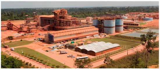
Figure 1.
Hydro’s Paragominas bauxite mine in Pará, Brazil [22].

Figure 2.
Bauxite-mining operations at Hydro’s Paragominas mine in Pará, Brazil [23].
This study uses multi-year operational data provided by Hydro from the SAG mill at the Paragominas site (Pará, Brazil), as shown in Figure 3. The dataset comprises approximately four years of time-stamped measurements spanning 2021 through to early 2025. Telemetry was sourced directly from Hydro’s plant historian based on the AVEVA PI System. For reproducibility and to preserve native timestamps and tag metadata, we ingested the data programmatically from MATLAB via Industrial Communication Toolbox, which provides a PI Data Archive interface for tag discovery and historical reads. Core electrical and mechanical channels include the three line voltages (phases 1–3), motor current, motor rotational speed, cumulative energy consumption, and lubrication-system temperatures for both the clean. and dirty-oil circuits. Together, these variables characterize drive loading, duty cycle, and the thermal behavior of bearings and lubrication, signals routinely used as condition indicators for large rotating assets. To support supervised learning and operational interpretation, Hydro also supplied a structured event log covering the same period. Each entry records downtime with start and end timestamps, duration and an assigned causal category including mechanical, electrical, planned maintenance, or external power loss. This log enables alignment of telemetry with ground-truth outcomes for fault detection and for constructing run-to-failure trajectories.
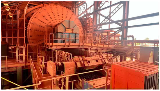
Figure 3.
SAG mill at Hydro’s Paragominas bauxite-processing plant.
Using MATLAB’s Industrial Communication Toolbox, we established a direct interface to the AVEVA PI System and imported the SAG mill unit’s time-stamped data into MATLAB. As summarized in Table 1, the dataset includes phase voltages (phases A–C), motor speed, clean- and dirty-oil temperatures, and other relevant process variables. Records are available at a uniform 1 min cadence beginning at 00:00 on 1 January 2021, providing a continuous history for subsequent preprocessing and modeling. The PI System recorded sensor measurements at a one-minute interval. This resolution was adequate for our analysis because the key health indicator was temperature, whose degradation trend evolves gradually and does not require high-frequency sampling. The one-minute interval was therefore sufficient to capture relevant dynamics for RUL estimation in this case. In other contexts, particularly when vibration or high-frequency current signals are dominant health indicators, smaller sampling intervals would be necessary to ensure early fault detection.

Table 1.
Sample view of the SAG mill dataset imported from the AVEVA PI System. For brevity, only representative columns are displayed (data time, voltage phase 1–3, feeding rate, energy consumption, current, active power, and speed). The full table contains 33 variables and 2,226,240 1 min records starting from 1 January 2021 00:00.
Table 2 summarizes the four-year SAG mill event log, including start/end time, duration, area/discipline, equipment, action, cause, and effect. We use this log as ground truth to mark failures and assemble a pretraining run-to-failure table for training; the spreadsheet itself is not imported into MATLAB.
Table 2.
Partial event log for SAG mill showing maintenance and failure records from 2021 to 2025 including start/end time, duration, area/discipline, equipment, action, cause, and effect.
3. Data Preprocessing
Before model development, the historian data was rigorously preprocessed to obtain a clean, analysis-ready corpus. Noninformative intervals such as plant-wide power losses, communication dropouts, and scheduled or unscheduled maintenance windows were identified from the event logs and masked to prevent spurious labels. We also addressed instrumentation artifacts, including noise bursts, stuck sensors, transient misreads, and gaps that occurred during these periods. The resulting workflow aligned all tags on the 1 min grid, reconciled units, removed values outside physically plausible bounds, detected outliers using robust statistics, and imputed short gaps with interpolation to preserve dynamics while avoiding information leakage.
As illustrated in Figure 4, the temperature of a specific subsystem typically resides within an operational envelope of ~35–65 °C; the isolated spike near 200 °C is a sensor artifact rather than a true failure. Such points are automatically flagged as outliers and replaced with interpolated estimates (using MATLAB’s Statistics and Machine Learning Toolbox), while longer maintenance intervals are retained as masked segments. This procedure yields contiguous run-to-failure sequences suitable for training and validating predictive models in the subsequent stage.
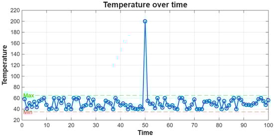
Figure 4.
Example outlier in the motor temperature data. The blue line represents the measured temperature over time. The green dashed line indicates the maximum operating margin (65 °C) and the red dashed line indicates the minimum operating margin (35 °C). The single spike at ~200 °C is identified as an outlier outside the normal operating range.
Figure 5 shows the motor current over four years. As can be observed from this figure, when the current drops to zero, the mill is stopped, and using the event log, we can tag the reason for each stop. If a stop is due to an external power loss, maintenance, a communication issue, or a bad sensor value, we mark it as non-failure and replace those points as an outlier and with interpolation. If a stop is due to a mechanical/electrical failure, we keep it and split the data into run-to-failure segments to use for training of the next step. Outlier removal was applied only to shutdowns or anomalies not related to equipment degradation, such as external energy disconnections or faulty sensor readings. For example, in the current signal (Figure 5 and Figure 6), the expected normal operating value is around 140 A. After outlier removal, the accepted range of 130–150 A reflects stable operation within the normal working regime. Interpolation was therefore limited to restoring missing values within these regime-consistent bounds, preventing the creation of artificial degradation trends.
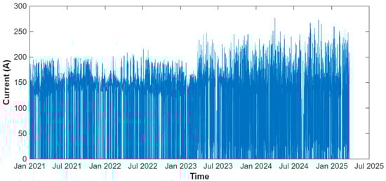
Figure 5.
Four-year current profile (1 min sampling) for unit SAG mill. The intermittent segments with zero current correspond to periods of scheduled or unscheduled shutdowns, as well as equipment failure events. External power outages, communication failures, and sensor noise are considered outliers that should be replaced.
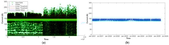
Figure 6.
Cleaning steps for the current signal. (a) Raw data with thresholds: green circles (o) represent the input current data, black crosses (x) indicate detected outliers, the red lines denote the lower and upper thresholds, and the blue line indicates the center value. Flat zero-current intervals correspond to downtimes. (b) Cleaned current series after outlier interpolation (blue line); downtimes remain as NaN gaps, which are later used to segment run-to-failure records.
Figure 6a marks two kinds of non-normal points in the current signal: outliers (isolated spikes) and downtimes (zero-current stretches). We replace outliers using interpolation, so the trend is preserved, but we do not fill downtimes because they represent failures. In Figure 6b, the outliers have been replaced, while downtimes are kept as NaN (Not-a-Number) gaps. These NaN gaps later define the boundaries of the run-to-failure segments used to build the training table.
We apply the same cleaning steps to all 27 tags on the main table. Among these signals, the clean-oil and dirty-oil temperatures carry the most diagnostic value and are therefore our primary candidates for a health indicator curve. As can be observed in Figure 7, after each restart, they begin at their lowest values and, as the mill runs, they rise steadily and often reach local peaks near a stop or failure of machine. We use these two temperatures as primary health indicator signals and later segment them into run-to-failure rows for model training. In addition, the dirty-oil temperature is about 4 °C warmer than the clean-oil temperature throughout the period, reflecting expected heat pickup in the return line. Despite this offset, the two series exhibit the same oscillating pattern within each run.
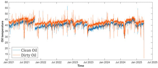
Figure 7.
Clean- and dirty-oil temperature curves.
At this stage, we aim to build a training set to learn a condition indicator (CI) and estimate the RUL, as illustrated in Figure 8. In this curve, the horizontal axis represents the lifetime of the machine, while the vertical axis corresponds to the CI. Each operating segment may result in different RUL estimates depending on the current condition. The strategy is to use the available historical data to identify the most suitable predictive model for the system. Once the model is established, it can be continuously updated with newly collected data. As the system approaches failure, the model provides increasingly accurate RUL predictions.
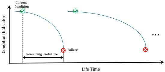
Figure 8.
Condition indicator versus Lifetime within a run; RUL is the time remaining from the current condition to failure.
We grouped the four-year history into run-to-failure segments using the downtime gaps as boundaries and focused on one specific recurring electrical failure. In the maintenance logs, these failures were consistently traced to repeated faults in the Liquid Rheostat Starter (LRS) circuit of the SAG mill drive, which caused protective trips and motor shutdowns. To capture the degradation trajectory leading to these events, we required sensor signals with clear monotonic behavior until failure. As mentioned before, among the available measurements, the clean- and dirty-oil temperatures displayed a consistent upward trend across runs, reaching peak values near failure events. This pattern justified their selection as primary condition variables and provided the diagnostic foundation for constructing the health indicator and training the predictive model. For each run, we kept all 33 cleaned tags and created a matching Lifetime vector that counts the minutes remaining until the failure at the end of that run (the last sample is zero). The result is the dataset in Table 3: it has 24 rows and two columns; Features and Lifetime. The Features entry for each row is an Ni × 33 table containing the synchronized signals including currents, phase voltages, active power, motor speed, clean- and dirty-oil temperatures, etc. The Lifetime entry is an Ni × 1 vector giving the minutes-to-failure for the same samples. For example, the first run contains 80,016 min samples, which means that failure occurred exactly at 80,016 min in that segment.
Table 3.
Run-to-failure training set for the recurring electrical failure mode (2021–2025). Each row represents one run. Features: cleaned, synchronized time series for 33 tags Ni × 33, Lifetime: minutes-to-failure for the same samples Ni × 1.
To develop the predictive model, we divided the dataset into training and testing/validation subsets. Here, for example, the first 20 rows of run-to-failure records were selected to train the model and capture the degradation patterns of the condition indicator. The remaining four rows were reserved for testing and validation. In this study, the availability of 24 run-to-failure cases was sufficient to ensure the accuracy of the similarity-based model. Nevertheless, in situations where only a limited number of run-to-failure events is available, the predictive model cannot provide reliable accuracy, and in this case, digital twins could be implemented to generate additional synthetic scenarios. Another limitation is that the method requires sensor variables that show clear degradation trends, such as the oil temperature signal that increased consistently until failure in our dataset. In the absence of such indicators, finding a predictive model will be challenging. Despite these constraints, the workflow is generalizable to a wide range of industrial equipment, provided that adequate degradation data or simulated trajectories are accessible.
4. Predictive Model and Health Indicator
Three sensors can be selected to serve as condition variables, while the remaining sensors were designated as data variables. As illustrated in Figure 9, two temperature signals were chosen as condition variables due to their strong correlation with system degradation. In addition, three other signals were selected as data variables to capture the operational context and complement the condition-monitoring process. This distinction between condition and data variables is essential for building a robust model, as it allows the predictive algorithm to focus on the most informative features while still considering the influence of auxiliary signals.
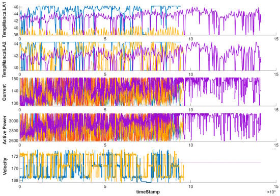
Figure 9.
Visualization of selected sensor signals used in the modeling process. Two temperature measurements (TempMancaLA1 and TempMancaLA2) were chosen as condition variables, while current, active power, and velocity were selected as data variables. Among all available run-to-failure cases, we selected four representative cases for illustration, and the plots show these signals across the chosen cases. Different colors represent the four run-to-failure cases, and the same color is used consistently across all subplots.
To ensure comparability of the signals and mitigate scale differences among the sensor measurements, we performed a normalization procedure grouped by working regimes. Specifically, for each sensor, the mean and standard deviation were computed within each operating regime identified in the previous section. This grouping ensures that normalization reflects the local operating context rather than global averages, thereby enhancing the sensitivity of the condition indicators to regime-specific variations. The normalized values were then obtained by subtracting the regime-specific mean and dividing by the corresponding standard deviation.
In addition to regime-wise normalization, a cluster-based normalization approach was also employed. First, the operating points of each sample were grouped into clusters representing distinct working regimes. For each cluster, the mean and standard deviation of every sensor measurement were computed. During normalization, each sample was assigned to its nearest cluster center based on the Euclidean distance to the operating points. The sensor measurements were then standardized by subtracting the corresponding cluster mean and dividing by the cluster standard deviation. To avoid instability, if the standard deviation of a cluster was close to zero, the normalized sensor measurement was set to zero. This procedure ensures that the normalization process is sensitive to local operating conditions while suppressing signals that do not contribute to meaningful variability, thus improving the robustness of the RUL estimation.
After applying the normalization procedure based on working regimes, the sensor signals become more comparable across different operating conditions. This regime-aware scaling removes the bias introduced by varying operating points and highlights the underlying degradation patterns. To account for varying operating regimes, the signals were first grouped by clustering. We applied the k-means algorithm to the operating condition variables, which effectively separated the data into distinct machine regimes. The optimal number of clusters was determined using the silhouette criterion, ensuring compact and well-separated groups. Normalization was then performed within each cluster, aligning the signals by regime and removing bias due to shifts in operating conditions. This procedure ensured that the degradation trends used for RUL estimation were comparable across different operating states.
As illustrated in Figure 10, the normalized data reveals clearer trends in several condition-related measurements, which were previously masked by regime-dependent variability. These revealed degradation trajectories are critical for constructing reliable condition indicators and improving the accuracy of RUL estimation.
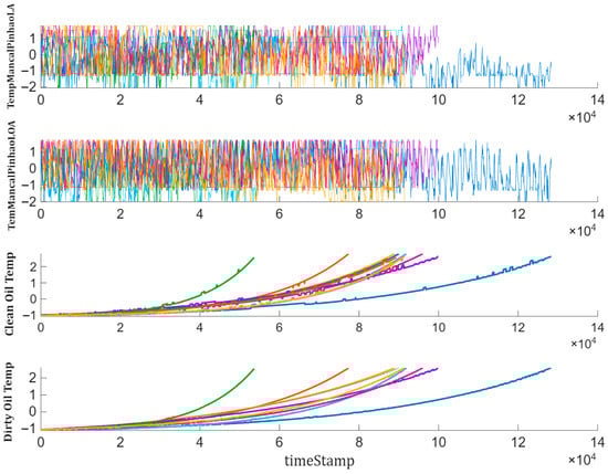
Figure 10.
Sensor measurements after normalization by working regime.
In selecting condition variables, we evaluated the standard condition indicator quality metrics, including monotonicity, trendability, and prognosability, across all normalized signals. Monotonicity ensures a consistent increase or decrease toward failure; trendability verifies that runs share a similar degradation shape; prognosability checks separation at end-of-life. Features were retained only when they scored well jointly; in our data, the clean- and dirty-oil temperatures satisfied these criteria across runs, justifying their use as primary condition variables. When no signal exhibits adequate monotonicity/trendability/prognosability, the reliability of similarity-based RUL estimates is expected to diminish.
To evaluate the trendability of the available sensor signals, we fitted a linear degradation model to each normalized measurement. The linear mapping of the health indicator from 1 (healthy) to 0 (failure) follows the standard similarity-based prognostic framework [23,24]. This representation does not imply that the underlying physical degradation process itself is linear; rather, it provides a normalized reference scale for comparing run-to-failure trajectories. Because similarity models operate on the full trajectory shape, they remain capable of accommodating nonlinear degradation behaviors across different runs. The fitted model provided an estimate of the slope, which quantifies the monotonic change in the signal over time. Sensor measurements with higher slope magnitudes were ranked as more trendable since they exhibited stronger and more consistent degradation patterns. Based on this ranking, the most trendable variables were selected for constructing a condition indicator, which will serve as the basis for RUL prediction. These variables are presented in Figure 11.
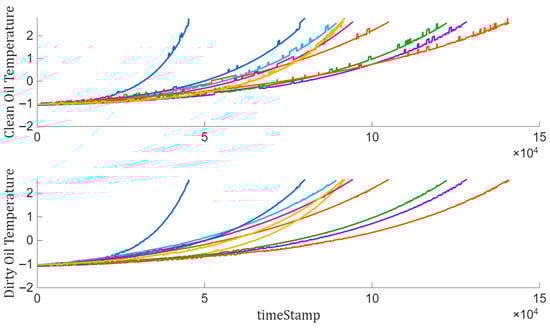
Figure 11.
Visualize the selected trendable sensor measurements.
In predictive maintenance, three main classes of models are typically considered for RUL estimation: survival models, degradation models, and similarity-based models. Survival models rely on population-level statistics and require the collection of failure time data across multiple systems, making them useful when individual degradation signals are unavailable. Degradation models assume that condition indicators follow specific parametric trends (e.g., exponential or linear) and estimate RUL by extrapolating these trends to a failure threshold. Similarity-based models, in contrast, exploit complete run-to-failure trajectories by comparing partially observed degradation profiles of a unit with historical trajectories from similar systems. Since our dataset included full time-series measurements from healthy state to failure, similarity-based modeling was the most appropriate choice, enabling direct use of historical degradation patterns for RUL prediction. This part focuses on fusing the selected sensor measurements into a single health indicator, which serves as the basis for training a similarity-based prediction model. All run-to-failure trajectories are assumed to start in a healthy condition. As can be observed in Figure 12, the initial health condition is assigned to a value of 1, while the failure state is assigned to a value of 0. Between these two points, the health condition is assumed to degrade linearly from 1 to 0 over time. This linear degradation profile is then used to guide the fusion of the sensor measurements, ensuring that the constructed health indicator consistently reflects the progression from healthy operation to failure.
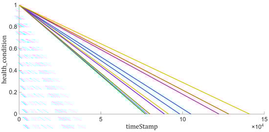
Figure 12.
Visualization of health condition.
The health condition of all ensemble members is depicted in Figure 13 with different rates of deterioration depending on the operating conditions. To capture the relationship between sensor signals and health progression, a linear regression model was fitted using the most trendable sensor measurements as regressors.
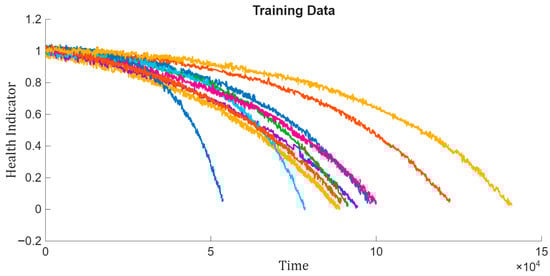
Figure 13.
Visualization of health indicator for training data.
To assess the generalization capability of the proposed method, the same operations were applied to the validation dataset, which consisted of the four run-to-failure trajectories previously separated for testing. The validation data was first subjected to regime-based normalization using the regime statistics obtained from the training set. Subsequently, the same sensor fusion process was applied to construct the health indicator. This ensured that the validation data followed an identical preprocessing pipeline, allowing for a consistent evaluation of model performance. The resulting health indicator trajectories are shown in Figure 14.
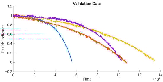
Figure 14.
Visualization of health indicator for validation data.
5. Estimate the RUL and Deploy the Model
In this work, we tested regression, survival, and similarity-based RUL learners. The survival model requires specific signals and hazard function parameterization; however, with the available data, the results did not converge. Regression learners assume predefined functional forms for degradation, which limited their performance given the variability in the dataset. In contrast, the similarity-based learner could directly leverage the complete run-to-failure trajectories, leading to stable and accurate RUL predictions. For these reasons, the similarity-based approach was selected for detailed implementation and analysis in this study.
Following the similarity-based prognostics· framework proposed by Wang et al. [24] and later extended in the work [25], the distance between two degradation trajectories is computed using the L1-norm of the residual, and the similarity score is defined through an exponential transformation of the squared distance [26]:
The number of nearest neighbors k is a key hyperparameter in the similarity-based RUL model. In our implementation, k was determined automatically by cross-validation, selecting the value that minimized the prediction error across the training set. This procedure balances bias and variance, ensuring that the RUL estimate is influenced by an appropriate neighborhood size rather than an arbitrarily chosen parameter. We also confirmed that small variations in k around the selected value did not significantly alter the results, indicating that the model’s performance is robust with respect to this choice. To evaluate the performance of the residual-based similarity RUL model, the prediction was tested on partial observation windows of the validation trajectories. Specifically, 50%, 70%, and 90% of each run-to-failure trajectory were used as input to the model, and the RUL was estimated at each truncation point. This approach emulates real-world scenarios where only a portion of the degradation trajectory is available and allows us to assess the accuracy and robustness of the model at different stages of equipment degradation. For the first evaluation scenario, the validation data was truncated at the first breakpoint, corresponding to 50% of its lifetime. The truncated trajectory was then used as input to the residual similarity model. The model identified the nearest neighbors from the training set based on the residual distance metric, and these were used to estimate the RUL. The validation trajectory is truncated at 50% and its nearest neighbors are visualized in Figure 15, illustrating how the model aligns the partially observed degradation pattern with historical trajectories to generate RUL predictions. The run-to-failure trajectories in the dataset span a wide range of durations, from approximately 45,000 to 141,000 min. To mitigate potential bias toward longer or shorter lifespans, the similarity-based model compares aligned residual trajectories rather than absolute times. During validation, each trajectory is truncated at the chosen observation window (50%, 70%, or 90%), and similarity is evaluated only on the overlapping portion. This ensures that similarity depends on the degradation pattern rather than total operating time, preventing systematic favoring of trajectories with specific durations.
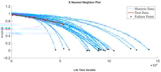
Figure 15.
Validation trajectory truncated at 50% of its lifetime and the corresponding nearest neighbors identified by the residual similarity model.
Now, we can visualize the estimated RUL compared to the true RUL, along with the probability distribution of the estimation. These results are depicted in Figure 16. As we can see in this figure, the distance between the estimated RUL and the true RUL is calculated as 53,403.4−38,934 = 14,469 min. Converting this difference into days gives 14,469/1440 ≈ 10.05 days, which means there is approximately a 10-day difference between the actual failure time and the predicted RUL. Hence, a noticeable error appears between the estimated and actual RUL when the system is in its mid-life condition.
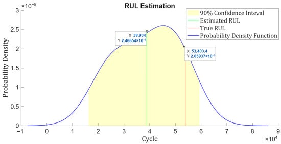
Figure 16.
Estimated RUL versus true RUL for the validation trajectory truncated at 50% of its lifetime, including the probability density function and the 90% confidence interval of the prediction.
For the next evaluation step, the validation data was truncated at the second breakpoint, corresponding to 70% of the lifetime. The residual similarity model was then applied to estimate the RUL based on the partially observed trajectory. The results of this evaluation are shown in Figure 17.

Figure 17.
Validation trajectory truncated at 70% of its lifetime and the corresponding nearest neighbors identified by the residual similarity model.
This evaluation also provides a visualization of the estimated RUL relative to the true RUL, as well as the probability distribution that characterizes the prediction uncertainty that can be seen in Figure 18.
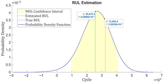
Figure 18.
Estimated RUL versus true RUL for the validation trajectory truncated at 70% of its lifetime, including the probability density function and the 90% confidence interval of the prediction.
As illustrated in Figure 18, the difference between the predicted RUL and the actual RUL is calculated as 31,850.4−25,672.3 = 6178.1 min. Converting this into days yields 6178.1/1440 ≈ 4.3 days which indicates that the predicted RUL deviates from the actual failure time by approximately 4.3 days.
As more data becomes available, the accuracy of RUL estimation improves. For the third evaluation scenario, the validation data was truncated to 90% of its lifetime. The residual similarity model was then applied to this partial trajectory to estimate the RUL, providing a more reliable prediction at this late stage of degradation. This result can be observed in Figure 19.
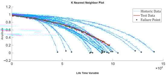
Figure 19.
Validation trajectory truncated at 90% of its lifetime and the corresponding nearest neighbors identified by the residual similarity model.
As shown in Figure 20, the gap between the predicted RUL and the actual RUL is obtained as 10,297.4−5838.03 = 4459.4 min. When this value is converted into days, it results in 4459.4/1440 ≈ 3.1 days, indicating that the predicted RUL differs from the actual failure time by about 3.1 days. The result shows that when the machine approaches failure, the RUL estimation becomes even more accurate in this case.
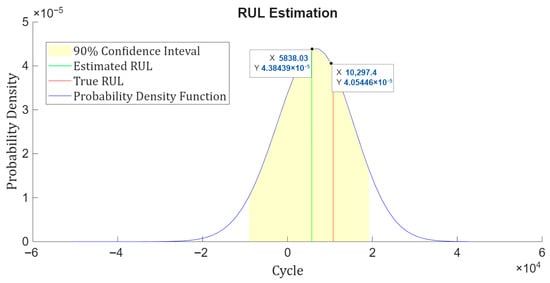
Figure 20.
Estimated RUL versus true RUL for the validation trajectory truncated at 90% of its lifetime, including the probability density function and the 90% confidence interval of the prediction.
In addition to reporting absolute error in days, standardized prognostic metrics can also be derived from the predicted and true RUL values. Relative accuracy (RA) at a prediction instant k is defined as follows:
which normalizes the error relative to the true RUL. Cumulative relative accuracy (CRA) averages this performance across the entire prediction horizon and is expressed as follows:
where N is the number of prediction points. The prognostic horizon (PH) is defined as the earliest time index k from which the predictions remain within a specified error bound ϵ:
These metrics are widely recognized for evaluating prognostic performance [27].
To enable practical use of the developed predictive model, we designed a MATLAB App that can automatically receive newly acquired data daily and apply the trained model to update the RUL estimation of the system. To enhance usability and ensure accessibility for end-users, the application was deployed through the MATLAB Web App Server. This deployment strategy allows the App to be executed directly from a standard web browser without requiring access to the MATLAB environment or the source code. Consequently, users can interact with the application seamlessly from various devices in the same network, such as smartphones, tablets, or personal computers, simply by opening a browser interface. This approach ensures that RUL updates are readily available in real time with minimal technical requirements. Figure 21 illustrates the deployed App operating within a web browser environment.
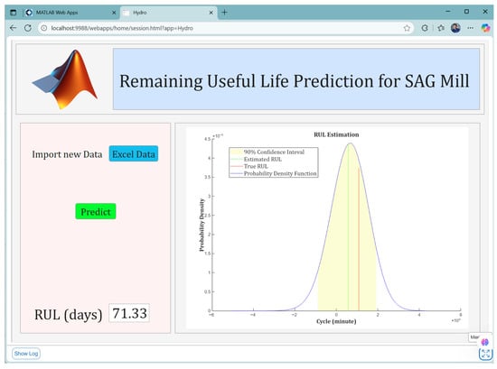
Figure 21.
Graphical interface of the RUL prediction application for the SAG Mill, deployed through MATLAB Web App Server. The App enables users to import new operational data, execute RUL estimation with a single command, and visualize results in terms of probability density function, estimated RUL, true RUL, and associated 90% confidence interval, all directly accessible from a web browser.
6. Conclusions
In this study, a complete workflow for data-driven RUL prediction was developed and validated. Starting with run-to-failure datasets, we first performed regime-based normalization, which successfully eliminated operating condition biases and revealed clear degradation trends in the sensor signals. From these normalized signals, the most trendable variables were identified using slope-based ranking of linear degradation models. These selected variables were then fused into a single health indicator, mapped from 1 (healthy) to 0 (failure), to serve as the basis for predictive modeling.
A residual similarity model was subsequently trained using ensemble members of the training dataset. This approach leveraged polynomial fitting of degradation trajectories, residual-based distance metrics, and exponential similarity scoring to identify the nearest neighbors in the training set for each validation case. The resulting probability distribution of RUL from the nearest neighbors allowed for robust estimation of failure times with associated confidence intervals.
Evaluation on the validation data with using truncation at 50%, 70%, and 90% of the lifetime demonstrated the progressive enhancement in prediction accuracy as more data became available. At earlier stages, the estimation errors were relatively larger due to less distinct degradation trends, but these errors decreased significantly as the system approached failure. For instance, the difference between predicted and actual RUL was approximately 10 days at 50% lifetime, 4.3 days at 70% lifetime, and reduced further to about 3.1 days at 90% lifetime. This confirms that the model is capable of capturing degradation dynamics and providing reliable RUL predictions, particularly in later stages of equipment life.
Finally, to facilitate practical application, we implemented the developed methodology into a MATLAB App. This application can receive new data in real time, apply the preprocessing and similarity-based model, and estimate the best RUL for the monitored system. Moreover, the app can be deployed through a MATLAB Web App Server, enabling end users to easily apply the model to new datasets without requiring deep technical expertise. This integration ensures that the proposed approach can be readily deployed for predictive maintenance in industrial environments.
Author Contributions
Data curation, M.D. and G.R.; formal analysis, M.D. and X.C.; investigation, M.D.; methodology, J.F. and V.A.; project administration, J.F.; resources, G.R.; software, M.D., X.C., V.A., E.L., C.M., C.d.R.I., M.R. and F.R.P.; supervision, J.F. and V.A.; validation, M.D., E.L., C.M. and C.d.R.I.; visualization, V.A.; writing—original draft, M.D.; writing—review and editing, M.D., G.R., X.C., E.L., C.M., C.d.R.I. and L.S. All authors have read and agreed to the published version of the manuscript.
Funding
This research received no external funding.
Data Availability Statement
The data presented in this study is available on request from the corresponding author. The data is not publicly available due to confidentiality agreements with Hydro Company.
Conflicts of Interest
Authors Mehdi Dehghan, Jean Franco, Ximena Cubillos, Vinícius Antunes, Eduardo Lima, Calequela Manuel, Christian da Rocha Iardino, Marco Reis, Fabio Reis Pereira, and Layhon Santos were employed by Opencadd Advanced Technology. Author Gilmar Rios was employed by Hydro. The authors declare that the research was conducted in the absence of any commercial or financial relationships that could be construed as a potential conflict of interest.
References
- Molęda, M.; Małysiak-Mrozek, B.; Ding, W.; Sunderam, V.; Mrozek, D. From Corrective to Predictive Maintenance—A Review of Maintenance Approaches for the Power Industry. Sensors 2023, 23, 5970. [Google Scholar] [CrossRef] [PubMed]
- Simard, S.R.; Gamache, M.; Doyon-Poulin, P. Current Practices for Preventive Maintenance and Expectations for Predictive Maintenance in East-Canadian Mines. Mining 2023, 3, 26–53. [Google Scholar] [CrossRef]
- Rojas, L.; Peña, Á.; Garcia, J. AI-Driven Predictive Maintenance in Mining: A Systematic Literature Review on Fault Detection, Digital Twins, and Intelligent Asset Management. Appl. Sci. 2025, 15, 3337. [Google Scholar] [CrossRef]
- Dayo-Olupona, O.; Genc, B.; Celik, T.; Bada, S. Approaches to Predictive Maintenance in Mining Industry: An Overview. Resour. Policy 2023, 86, 104291. [Google Scholar] [CrossRef]
- Nobahar, P.; Xu, C.; Dowd, P.; Shirani Faradonbeh, R. Exploring Digital Twin Systems in Mining Operations: A Review. Green Smart Min. Eng. 2024, 1, 474–492. [Google Scholar] [CrossRef]
- Miñón, R.; López-De-Armentia, J.; Bonilla, L.; Brazaola, A.; Laña, I.; Palacios, M.C.; Mueller, S.; Blaszczak, M.; Zeiner, H.; Tschuden, J.; et al. A Multi-Level IIoT Platform for Boosting Mines Digitalization. Future Gener. Comput. Syst. 2025, 163, 107501. [Google Scholar] [CrossRef]
- Hermosilla, R.; Valle, C.; Allende, H.; Aguilar, C.; Lucic, E. SAG’s Overload Forecasting Using a CNN Physical Informed Aproach. Appl. Sci. 2024, 14, 11686. [Google Scholar] [CrossRef]
- Ghasemi, Z.; Neumann, F.; Zanin, M.; Karageorgos, J.; Chen, L. A comparative study of prediction methods for semi-autogenous grinding mill throughput. Miner. Eng. 2024, 205, 108458. [Google Scholar] [CrossRef]
- Ghasemi, Z.; Neshat, M.; Aldrich, C.; Zanin, M.; Chen, L. An integrated intelligent framework for maximizing SAG mill throughput: Incorporating expert knowledge, machine learning and evolutionary algorithms for parameter optimization. Miner. Eng. 2024, 212, 108733. [Google Scholar] [CrossRef]
- Pinto, T.; da Silva, M.T.; Raffo, G.V.; Euzébio, T.A.M. Specific energy reduction in a semi-autogenous grinding mill circuit by an automatic control system. Sci. Rep. 2025, 15, 21398. [Google Scholar] [CrossRef] [PubMed]
- McCoy, J.T.; Auret, L. Machine Learning Applications in Minerals Processing: A Review. Miner. Eng. 2019, 132, 95–109. [Google Scholar] [CrossRef]
- Fu, Y.; Aldrich, C. Flotation Froth Image Recognition with Convolutional Neural Networks. Miner. Eng. 2019, 132, 183–190. [Google Scholar] [CrossRef]
- MathWorks. What Is Predictive Maintenance? MATLAB & Simulink. Available online: https://www.mathworks.com/discovery/predictive-maintenance.html (accessed on 26 August 2025).
- Sbárbaro, D.; del Villar, R. (Eds.) Advanced Control and Supervision of Mineral Processing Plants; Series Advances in Industrial Control; Springer: London, UK, 2010. [Google Scholar] [CrossRef]
- Légaré, B.; Bouchard, J.; Poulin, É. A modular dynamic simulation model for comminution circuits. IFAC-PapersOnLine 2016, 49, 19–24. [Google Scholar] [CrossRef]
- Liu, Y.; Spencer, S. Dynamic simulation of grinding circuits. Miner. Eng. 2004, 17, 1189–1198. [Google Scholar] [CrossRef]
- Bono, F.M.; Cinquemani, S.; Chatterton, S.; Pennacchi, P. A Deep Learning Approach for Fault Detection and RUL Estimation in Bearings. In Proceedings of the In NDE 4.0, Predictive Maintenance, and Communication and Energy Systems in a Globally Networked World SPIE, Long Beach, CA, USA, 6 March–11 April 2022; Volume 12049, p. 1204908. [Google Scholar] [CrossRef]
- Shaheen, M.A.; Németh, I. Integration of Maintenance Management System Functions with Industry 4.0 Technologies and Features—A Review. Processes 2022, 10, 2173. [Google Scholar] [CrossRef]
- Garcia, J.; Rios-Colque, L.; Peña, A.; Rojas, L. Condition Monitoring and Predictive Maintenance in Industrial Equipment: An NLP-Assisted Review of Signal Processing, Hybrid Models, and Implementation Challenges. Appl. Sci. 2025, 15, 5465. [Google Scholar] [CrossRef]
- ISO 13374-1:2003; Condition Monitoring and Diagnostics of Machines—Data Processing, Communication and Presentation—Part 1: General Guidelines. ISO: Geneva, Switzerland, 2003.
- Panov, S.; Nikolov, A.; Panova, S. Review of Standards and Systems for Predictive Maintenance. Sci. Eng. Educ. 2021, 6, 65–73. [Google Scholar] [CrossRef]
- Norsk Hydro ASA. Paragominas Mine: Start-Up of Production: 2007; Nominal Capacity: 9.9 Mt; Production: 11.4 Mt/y. Available online: https://www.hydro.com/en/global/about-hydro/hydro-worldwide/americas/brazil/paragominas/paragominas-mine/ (accessed on 23 September 2025).
- Norsk Hydro ASA. Paragominas: Overview of Hydro’s Bauxite Operations (Annual Capacity: Nearly 10 Million t; Pipeline Transport; Employees: ~1,300 Permanent and ~350 Long-Term)”, Hydro. Available online: https://www.hydro.com/en/global/about-hydro/hydro-worldwide/americas/brazil/paragominas/ (accessed on 23 September 2025).
- Wang, T.; Yu, J.; Siegel, D.; Lee, J. A similarity-based prognostics approach for remaining useful life estimation of engineered systems. In Proceedings of the International Conference on Prognostics and Health Management (PHM 2008), Denver, CO, USA, 6–9 October 2008; IEEE: Piscataway, NJ, USA, 2008; pp. 1–6. [Google Scholar] [CrossRef]
- Doering, T.; Hishmeh, S.; Dodson, T.; White, A.; Eluru, P.; Padmanabhan, P. The KySat Space Express Sub-Orbital Mission Summary. In Proceedings of the 2008 IEEE Aerospace Conference, Big Sky, MT, USA, 1–8 March 2008; pp. 1–12. [Google Scholar] [CrossRef]
- Peng, Y.; Dong, M.; Zuo, M.J. Current status of machine prognostics in condition-based maintenance: A review. Int. J. Adv. Manuf. Technol. 2010, 50, 297–313. [Google Scholar] [CrossRef]
- Saxena, A.; Celaya, J.; Balaban, E.; Goebel, K.; Saha, B.; Saha, S.; Schwabacher, M. Metrics for Evaluating Performance of Prognostic Techniques. In Proceedings of the 2008 IEEE International Conference on Prognostics and Health Management (PHM), Denver, CO, USA, 6–9 October 2008; pp. 1–17. [Google Scholar] [CrossRef]
Disclaimer/Publisher’s Note: The statements, opinions and data contained in all publications are solely those of the individual author(s) and contributor(s) and not of MDPI and/or the editor(s). MDPI and/or the editor(s) disclaim responsibility for any injury to people or property resulting from any ideas, methods, instructions or products referred to in the content. |
© 2025 by the authors. Licensee MDPI, Basel, Switzerland. This article is an open access article distributed under the terms and conditions of the Creative Commons Attribution (CC BY) license (https://creativecommons.org/licenses/by/4.0/).