Multi-Bolt Structural Loosening Fault Identification Based on Black-Winged Kite Algorithm and CNN-GRU

Abstract

Wind turbines serve as core equipment for renewable energy development and utilization. Tower high-strength bolts are critical load-bearing components of wind turbines, making precise detection and early identification of their failures of significant importance. By addressing the challenges of extracting failure features from tower high-strength bolts and the insufficient generalization capability of traditional intelligent diagnostic models, this study achieves the precise detection and early identification of bolt-loosening failures. This study independently constructed a simulation platform to collect bolt vibration data and proposed a diagnostic model—BKA-CNN-GRU—based on a CNN-GRU architecture enhanced by the Black-winged Kite Algorithm (BKA). This approach enables precise detection and early identification of high-strength bolt-loosening failures. The specific research approach involved first establishing experimental conditions with varying bolt tightening levels to capture time-domain vibration signals. Subsequently, Fast Fourier Transform (FFT) was applied to convert these signals into frequency-domain data. Building upon this, BKA optimization was employed to refine key hyperparameters of the CNN-GRU model, thereby enhancing diagnostic performance. Experimental results demonstrate that, under the same dataset, the BKA-CNN-GRU model achieves an average accuracy of 99.31%, significantly outperforming comparison models such as CNN-GRU. Furthermore, the model exhibits robust performance and strong generalization capabilities under varying sample proportions and small-sample conditions.

1. Introduction

High-strength bolted connections serve as a critical method for assembling structural components in engineering applications, playing a pivotal role in large-scale steel structures. For instance, high-strength bolts within wind turbine towers bear the responsibility of transmitting dynamic loads such as wind forces, centrifugal forces, tensile stresses, and vibrations [1,2], ensuring the long-term reliable operation of wind turbines. However, the load-bearing performance of such connections is influenced by multiple factors. Inadequate preload can directly cause loosening while under multi-physics coupling conditions involving vibration, impact, thermal loads, and atmospheric corrosion [3,4]. In 2020, a wind farm in Hebei Province experienced a tower collapse due to the failure of 128 bolts in the tower connection, resulting in significant property damage [5]. This incident underscores the critical link between bolt stability and public safety, as well as societal stability. Such damage can degrade structural load-bearing capacity or lead to complete failure. Therefore, detecting and identifying bolt loosening and early-stage damage before structural failure occurs is crucial for preventing accidents and reducing maintenance costs. This has become a key research topic over the past decade in fields such as wind power generation [6], machinery [7], aerospace [8], and civil engineering. Advanced technologies like big data and artificial intelligence offer intelligent solutions to enhance detection accuracy and efficiency, ensure the safety of operations and maintenance personnel, and reduce costs.

Currently, the mainstream approach for monitoring the health status of wind turbine tower bolts involves real-time assessment through physical quantity sensing and intelligent data analysis. Among these, vibration signal analysis serves as the core technical pathway. This method deploys sensors to capture vibration signal responses at bolt connection points, indirectly reflecting bolt health through changes in structural vibration characteristics. However, its accuracy is susceptible to interference from complex environmental noise at the site. Therefore, raw data requires preprocessing such as filtering, normalization, principal component analysis [9], wavelet transform [10], Fast Fourier Transform (FFT) [11], and Gaussian oversampling techniques [12]. For instance, combining FFT and wavelet transform extracts frequency-domain energy distribution features, while time-domain statistics like kurtosis and root mean square (RMS) quantify nonlinear effects caused by loosening. To suppress noise, empirical mode decomposition (EMD) is commonly applied for adaptive noise reduction on raw signals. This method demonstrates significant advantages in analyzing nonlinear, non-stationary signals, effectively isolating high-frequency vibration characteristics associated with bolt loosening or fracture by decomposing complex signals into multiple intrinsic mode functions [13]. Notably, such vibration-based methods fall under sensor-based technologies. This category overcomes limitations of in situ detection and computer vision techniques—including susceptibility to environmental noise, time-consuming processes, and difficulty in detecting early-stage loosening—while offering markedly higher accuracy and reliability [14]. Current research explores integrating vibration-based methods with machine learning algorithms to detect and identify early-stage bolt loosening [15]. From a methodological perspective, vibration-based identification focuses on low-frequency signals (typically around kHz or 100 Hz), representing a holistic approach to detecting loosening damage. Existing methods for detecting hidden damage in multi-bolt connections often suffer from incomplete information due to neglecting either low-frequency or high-frequency bands. Therefore, effectively combining these methods with wave-based local damage detection techniques that focus on high-frequency signals can further enhance the efficiency of detecting loosening in multi-bolt connections.

In the health monitoring of wind turbine tower bolts, after data preprocessing, support vector machines [16], random forest algorithms, decision trees [17], and various neural networks can be employed to classify bolt conditions such as health, loosening, and fracture. In recent years, deep convolutional neural networks (CNNs) have emerged as a research hotspot in engineering. Their superior learning capabilities compared to traditional pattern recognition methods, coupled with the ability to automatically extract complex feature patterns without manual feature extractor design, offer a novel solution for intelligent identification of complex defects in steel bolt connections: Convolutional neural networks excel at processing images and two-dimensional data with local correlations. For instance, Li D et al. [18] constructed a CNN model to extract damage features from acoustic emission data, enabling the assessment of bolt looseness and wear mechanisms; Zhang Y et al. [19] trained and evaluated a region-based CNN model using a 300-image dataset capturing bolt tightening and loosening states, specifically addressing challenges in ultrasonic signal excitation and reception within complex regions where bolt positions are nonlinear; Tran DQ et al. [20] evaluated ultrasonic signal performance using deep convolutional neural networks and regression models; and Alif MAR et al. [21] compared CNNs, visual transformers, and compact convolutional transformers for analyzing bolt visual datasets, highlighting BoltVision’s effectiveness for train-specific safety inspections and resource-constrained edge devices. Long Short-Term Memory (LSTM) networks, as core components for temporal modeling, can directly process raw or lightly processed time-series signals and capture long-term data dependencies, making them suitable for continuous monitoring data from mechanical equipment. Zhao Jianjian et al. [22] trained a CNN-BiLSTM hybrid model using data such as tower vibration and tilt angle from wind turbine condition monitoring systems to achieve early warning of bolt acoustic conditions. Research on bolt-loosening detection combining deep learning with computer vision has also advanced. For instance, Zang et al. [23] employed CNNs for bolt detection and utilized the Fast Region-based Convolutional Network (Faster R-CNN) to solve regression problems for predicting bolt-loosening magnitude. Zhao et al. [24] employed smartphone-captured image datasets to detect loosening by measuring bolt head coordinates relative to top-mounted reference points and calculating rotation angles. However, this approach faces challenges including difficulty in early-stage detection, complex camera mounting in scenarios like automotive engines, and high computational costs of CNNs. Beyond these applications, Zhuo et al. [25] proposed a multi-bolt-loosening detection method based on acoustic signal support vector machine classification, capable of distinguishing bolt acoustic signals and environmental noise signals across different locations and loosening degrees. Zhao et al. [26] also developed a bolt-loosening angle recognition technique integrating deep learning and machine vision. However, deep learning heavily relies on large datasets for data-driven feature extraction. Furthermore, Li et al. [27] and Yu et al. [28] extended similar deep learning approaches to rail crack detection and structural damage identification in buildings, further validating its adaptability. As shown in

Table 1. Advantages and disadvantages of different combination methods.

Core Methodology	Methodological Superiority	Methodological Limitations
Vibration Signal + Traditional Machine Learning	Possesses multi-state classification capabilities with strong logical interpretability	Weak learning capabilities for high-dimensional complex data
Vibration Signal + Deep Learning	Possesses the capability to distinguish target signals from noise, enabling the prediction of structural component performance	Model cross-scenario generalization is constrained by structural types
Computer Vision + Deep Learning	Corrects geometric distortion in images, precisely locates targets, and enables visual status recognition	Detecting early-stage, minute changes in condition is challenging

, the advantages and disadvantages of the various method combinations proposed in the above studies are summarized.

Despite significant progress in the aforementioned research, traditional methods still suffer from reduced accuracy in noisy environments and poor generalization capabilities under complex operating conditions. Furthermore, early detection of bolt-loosening failures remains challenging. Therefore, this paper proposes a method for early detection and identification of bolt loosening in multi-bolt structures based on vibration signals combined with machine learning classifiers. This approach specifically addresses the characteristics of high-strength bolted connections in steel structures, such as those in wind turbine towers, which exhibit strong state concealment and high complexity. It also leverages the nonlinear contact vibration signals generated when high-strength bolts loosen. An experimental setup was designed: A connection component containing 12 high-strength bolts with varying degrees of loosening was used to simulate the circumferential layout of wind turbine tower bolts. Multiple operating conditions, including healthy and non-healthy states, were set up. Vibration data was collected under two motor operating speeds: 1000 rpm and 3000 rpm. During data processing, Short-time Fourier Transform was employed to extract features from the raw vibration data, completing the data preprocessing. Finally, by evaluating the performance of different machine learning classifiers, the BKA-CNN-GRU classifier with the highest accuracy was selected. Results demonstrated that this classifier not only detects the early stages of bolt loosening but also precisely identifies the location of loosened bolts. Ultimately, the goal of loosening detection based on vibration acoustic modulation signals from high-strength multi-bolt loosening was achieved.

The remainder of this paper is structured as follows. Section 2 details the theoretical foundation of the proposed method and the overall architecture of the CNN-GRU model. Section 3 provides a comprehensive explanation of the experimental implementation. Section 4 presents the model training results and related discussions. Section 5 summarizes the key findings of this research.

2. Theoretical Foundation

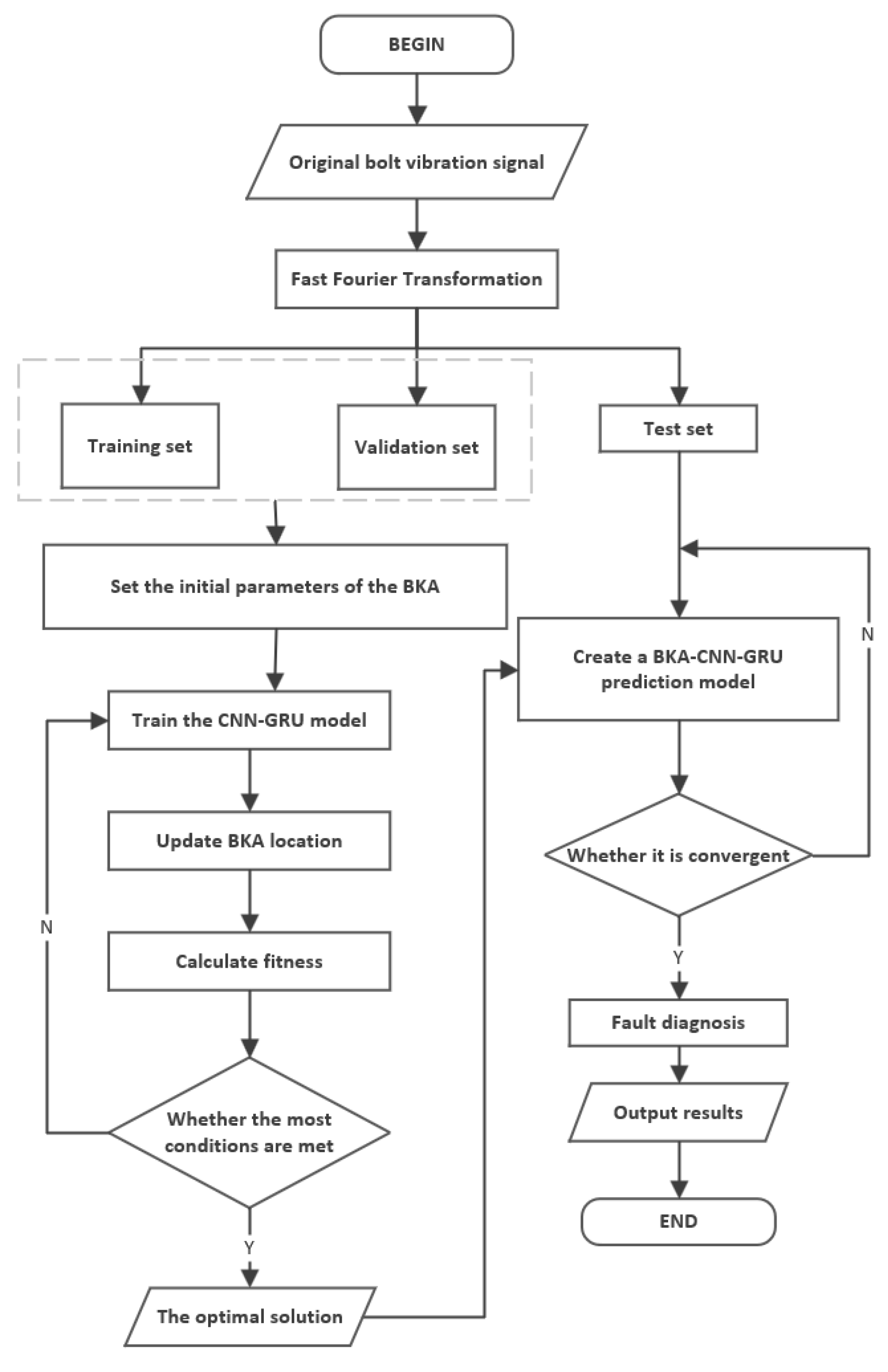
The flowchart of the proposed method in this study is shown in Figure 1. First, experimental data is collected. The collected bearing fault time-domain signals are converted into frequency-domain data using Fast Fourier Transform (FFT), and the data is divided into training, validation, and test sets. The Black-winged Kite Algorithm (BKA) [29] is employed to optimize parameters and train the CNN-GRU model, seeking the optimal solution. This process establishes the BKA-CNN-GRU prediction model, which performs fault diagnosis after convergence assessment and ultimately outputs results.

2.1. Feature Extraction

Feature extraction from raw vibration signals can be achieved through various methods: Ensemble Empirical Mode Decomposition (EEMD) [30], Singular Value Decomposition (SVD) [31,32], Continuous Wavelet Transform (CWT) [33], Variational Mode Decomposition (VMD) [34], Short-time Fourier Transform, etc. Feature extraction itself serves as the core link connecting raw data to model training in machine learning, a point reflected in numerous related studies. For instance, Zhao et al. [35] proposed a fault diagnosis method based on multi-input convolutional neural networks, using three convolutional kernels of different sizes to extract features of varying dimensions and completing fault classification via a Softmax classifier; Chen Yuhang et al. [36] achieved high accuracy in bearing fault diagnosis using the Fast Fourier Transform and CNN; and Chen Daijun et al. [37] proposed a rolling bearing fault diagnosis method based on VMDCWT-CNN, enabling effective signal feature extraction and precise damage severity diagnosis.

Building upon the aforementioned research, this paper proposes a method based on the Fast Fourier Transform (FFT) to address the requirement for feature extraction from bolt vibration signals. As an optimized algorithm of the Discrete Fourier Transform, the Fast Fourier Transform not only simplifies computational complexity and accelerates processing speed but also clearly reveals information in the frequency domain that remains unobservable in the time domain. Its specific principle is as follows: the Fast Fourier Transform (FFT), as an optimized algorithm for the Discrete Fourier Transform, not only simplifies computational complexity and accelerates processing speed but also clearly reveals information in the frequency domain that remains hidden in the time domain. Its specific mechanism is as follows: Sampling the original fault signal at frequency F_S with N sampling points yields N complex points after FFT. Each complex point corresponds to a frequency value, where the phase of each point represents the phase of that frequency component and the magnitude represents its amplitude. The expression represented by point n is

$$F_n=(n-1)\times \frac{F_s}{N}$$

(1)

The Discrete Fourier Transform expression for sequence x(n) = {x₀, x₁, …, x_N−1} is as follows:

$$\widehat{x}\left(k\right)={\displaystyle \sum _{n=0}^{N-1}x\left(n\right)e^{-\frac{2\pi }{N}nk}}$$

(2)

Here, e denotes the base of the natural logarithm, i represents the imaginary unit, and N indicates the number of sampling points; k = 0, 1 …, N−1.

2.2. Convolutional Neural Networks (CNNs)

In the field of deep learning, convolutional neural networks (CNNs) rank among the most renowned and widely applied algorithms [38]. First proposed as early as the 1960s [39], their primary advantage lies in their ability to automatically identify relevant features without human intervention [40]. Additionally, CNNs excel at tackling complex tasks, particularly in computer vision, where they effectively handle computationally intensive visual challenges [41]. Related applications span image classification [42], image recognition [43], object detection [44], and video processing [45]. Beyond this, CNNs extend into multiple other domains, including speech recognition [46], facial recognition [47], and natural language processing. Regarding CNNs’ advantages, Goodfellow et al. [48] further highlighted three core characteristics: equivalent representations, sparse interactions, and parameter sharing.

CNNs operate similarly to visual cortex cells as feedforward neural networks, composed of convolutional layers, pooling layers, and fully connected layers [49]. By alternately applying these layers, they extract features from raw sequential data, demonstrating a strong performance in image processing and recognition. The core of CNNs lies in the convolutional layer, where a convolution kernel slides across the input data, performing convolution operations within a local receptive field to extract features. Unlike traditional fully connected (FC) networks, CNNs utilize local connections and weight-sharing mechanisms to significantly reduce the number of parameters. This not only simplifies the training process but also accelerates network operation, thereby enhancing the efficiency of feature extraction.

The main components of the convolutional layer include the convolution kernel, layer parameters, and activation function. Convolution kernels perform the core operation: First, a kernel is overlaid on a local region of the input image, multiplying corresponding elements and summing them to produce an output value. Subsequently, the kernel slides across the image at a specified stride, performing pointwise convolution operations to generate a two-dimensional activation map [50]. This process repeats until the entire image is traversed, extracting features from the input data to produce a sequence of feature maps for subsequent processing [51]. Feature maps consist of multiple neurons. Each unit in the current convolutional layer’s feature map connects to a local region of the preceding layer’s feature map through a set of weights and an activation function. This process essentially maps effective features layer by layer through the neurons [49], calculated as follows:

$$l_t=\tanh \left(x_t\times k_t+b_t\right)$$

(3)

In the equation, l_t represents the output value after convolution; tanh denotes the activation function; x_t signifies the input vector; * indicates the convolution operation; k_t represents the weights of the convolution kernel; and b_t denotes the bias of the convolution kernel.

After performing convolution operations on the convolutional layer to extract data features, a pooling layer is added due to the high dimensionality of the extracted features. The pooling layer is responsible for reducing the dimensionality of the data, thereby lowering the feature map dimensions and parameter count, and reducing the network training cost. The max pooling expression is

$$P^{l\left(i,t\right)}=\underset{\left(j-1\right)c=1\le t\le jc}{\max }{a}^{l\left(i,t\right)}$$

(4)

In the formula, c represents the pooling width, and a^l(i,t) denotes the i activation value of the t feature map in layer l. After the pooling layer completes dimensional reduction and key feature selection, the convolutional neural network enters its core classification stage, primarily implemented by fully connected layers. The structural characteristic of fully connected layers is that each layer contains a large number of interconnected neurons. They can perform flattened feature map operations and, through deep processing of vector data, fully integrate global feature information, thereby enhancing the accuracy of the model’s classification results.

2.3. Gate Recurrent Unit (GRU)

The Gate Recurrent Unit (GRU) [52] is a simplified variant of the recurrent neural network (RNN) that addresses issues such as long-term memory and gradient vanishing during backpropagation in RNNs. Both the GRU and LSTM can resolve the vanishing gradient problem caused by convolutional neural networks (CNNs). However, compared to LSTM, the GRU features a more streamlined structure. By simplifying the network architecture and reducing training parameters, the GRU typically achieves a prediction performance comparable to LSTM while maintaining or even slightly improving predictive accuracy [53,54]. Leveraging this advantage, this paper adopts the GRU to capture the periodic characteristics of vibration signals.

Structurally, the GRU differs from LSTM, which contains three gating units. The GRU incorporates only a reset gate and an update gate internally. The update gate controls the extent to which prior information is retained in the current state, while the reset gate determines whether to associate prior information with the current state [55]. This design enables the GRU to selectively update and utilize information from previous time steps, thereby effectively capturing long-term dependencies in sequential data [56]. Specifically, the GRU calculates the states of these two gates by combining the hidden state passed from the previous time step with the input information at the current moment, thereby achieving information filtering and transmission. The update gate controls the extent to which the state information from the previous moment is carried into the current state. In other words, the update gate helps the model determine how much past information should be passed into the future—simply put, it is used to update memory. The calculation formula for the update gate is as follows:

$$z_t=\sigma \left(W_z\times \left[h_{t-1},x_t\right]\right)$$

(5)

$$h_t=\left(1-z_t\right)\times h_{t-1}+z_t\times h_t$$

(6)

In the formula, the closer the value of z_t is to 1, the more data is “memorized”; the closer the value of z_t is to 0, the more data has been “forgotten.” (1-z_t)*h_t−1 selectively “forgets” the hidden state from the previous time step, discarding irrelevant information from h_t−1. z_t*h_t represents further selective “memorization” of candidate hidden states, meaning it re-screens certain information from h_t, forgets some information passed from the previous layer, and incorporates some information from the current node’s input to form the final memory.

The reset gate controls the fusion of new inputs with previously stored memory states, a mechanism crucial for capturing short-term dependencies in time series. It determines the degree of historical forgetting based on current information, outputting values between 0 and 1 to represent the relative importance of past hidden states versus current inputs: outputs near 0 favor forgetting history, while outputs near 1 favor retaining it. The reset gate’s calculation formula is as follows:

$$r_t=\sigma \left(W_r\times \left[h_{t-1},x_t\right]\right)$$

(7)

$$h_t=\tanh \left(W\cdot \left[r_t\times h_{t-1},x_t\right]\right)$$

(8)

In the formula, W_r is a weight matrix that performs a linear transformation on the concatenated matrix of x_t and h_t−1. The product of the two matrices is then fed into the sigmoid function. The value of r_t can then be obtained. The smaller the value of r_t, the smaller the numerical value of the matrix after operation with h_t−1, and the smaller the value obtained after multiplication by the weight matrix. This indicates that more information needs to be forgotten in the previous time step. Conversely, this indicates a tighter coupling between the current input and historical memory. By calculating the update gate and reset gate according to the above formula, their outputs will control the degree of hidden state updates and historical information retention.

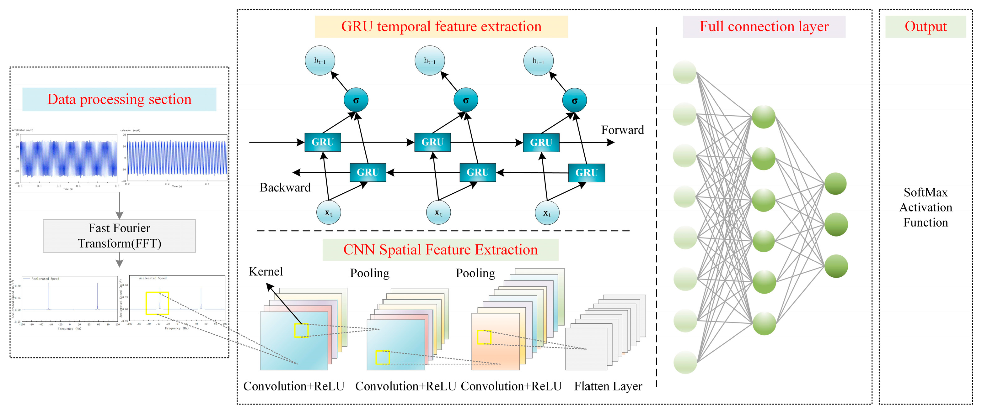
The CNN-GRU model constructed in this study adopts a dual-branch fusion architecture, as shown in Figure 2. First, the dataset is divided into training and validation sets and fed into the model. The GRU branch sequentially processes the data through GRU1, FC1 (fully connected layer 1), GRU2, and FC2 (fully connected layer 2) to extract temporal features. The CNN branch extracts spatial features through convolution operations, activation functions, and MaxPooling. Subsequently, the outputs from both branches are concatenated, integrated through FC3 (fully connected layer 3), and finally mapped to classification probabilities by the Softmax output layer to generate diagnostic results.

The CNN branch extracts spatial features, employing a structure comprising five convolutional layers and three fully connected layers. Convolution kernels extract local features from the data, while pooling layers reduce the dimensionality. A GRU (Gated Recurrent Unit) then processes temporal dependencies, and finally, fully connected layers complete the feature mapping and task output.

2.4. Black-Winged Kite Algorithm (BKA)

The Black-winged Kite Algorithm (BKA) is a novel intelligent optimization algorithm proposed by Wang et al. [57] in 2024. Inspired by the migratory and predatory behaviors of black-winged kites, it constructs a meta-heuristic optimization mechanism integrating global exploration and local exploitation by simulating the dynamic changes in their aerial search paths. Furthermore, by integrating the Cauchy mutation mechanism with the Leader guidance strategy, this algorithm effectively enhances global exploration efficiency and solution performance [58]. Furthermore, it maps the black kite’s biological behaviors into specific optimization strategies. For instance, its predatory behavior translates into fine-grained searches within solution space neighborhoods, while its group migration corresponds to the algorithm’s global exploration phase. Periodic spatial jumps prevent search stagnation, continuously opening up new solution regions [59].

Zhang et al. [60] combined a Black-winged Kite Algorithm based on logical chaotic mappings with the osprey optimization algorithm to address function evaluation and engineering layout problems. This approach effectively enhanced overall exploration intensity and computational efficiency through its capabilities for large-scale exploration and small-scale mining. Furthermore, Ma et al. [61] proposed a Black-winged Kite Algorithm incorporating optimal point sets, nonlinear convergence factors, and adaptive t-distribution for robotic parallel gripper design. This approach not only exhibits strong adaptability but also achieves more stable evaluation accuracy. Meanwhile, Xue et al. combined the Black Kite Algorithm with the Artificial Rabbit Optimization Algorithm to address function optimization problems. This algorithm prevents over-convergence and finds suitable solutions due to its excellent sustainability and universality [62]. Furthermore, Zhou et al. applied the Black Kite Algorithm with the Cosine Criterion for function optimization. Its outstanding reliability and adaptability enriched the information capacity of exploration and enhanced global convergence performance [63]. The Black-winged Kite Algorithm proposed by Rasooli et al. demonstrates an outstanding performance in clustering problems, combining applicability and cost-effectiveness to enhance exploration intensity, improve computational efficiency, and locate universally applicable solutions [64]. Although the improved Black-winged Kite Algorithm (BKA) demonstrates high reliability and flexibility in enhancing evaluation accuracy and collaborative efficiency, it still falls short in balancing local development and global exploration. Moreover, as indicated by the No Free Lunch (NFL) theorem, no single search method can solve all optimization challenges [65].

The specific process of optimizing BKA model parameters primarily involves three stages: population initialization, attack, and migration. The black-winged kite population is uniformly distributed with each kite assigned an initial position BK. The initialization of mathematical model X_i is expressed as

$$BK=\left[\begin{array}{cccc}B{K}_{1,1}& B{K}_{1,2}& \dots & B{K}_{1,d}\\ B{K}_{2,1}& B{K}_{2,2}& \dots & B{K}_{2,d}\\ ⋮& ⋮& ⋮& ⋮\\ B{K}_{p,1}& B{K}_{p,2}& \dots & B{K}_{p,b}\end{array}\right]$$

(9)

$$X_i=B{K}_{1b}+rand\left(B{K}_{ub}-B{K}_{1b}\right)$$

(10)

In the formula, d represents the dimension of the given problem; i is an integer between 1~pop, pop represents the number of black-winged kite populations, and X_i denotes the i-th candidate solution in the search space. BK_1b and BK_ub represent the lower bound and upper bound of the i-th black-winged kite in the j-th dimension; and rand is a random number between [0,1].

The attack behavior of the black-winged kite is employed to search for the global optimum solution, with its corresponding mathematical model being

$$y_{t+1}^{i,j}={\{}_{y_t^{i,j}+n\times \left(2r-1\right)\times y_t^{i,j},else}^{y_t^{i,j}+n\times \left(1+\sin r\right)\times y_t^{i,j},p<r}$$

(11)

$$n=0.05\times e^{-2\times {\left({\displaystyle \frac{t}{T}}\right)}^2}$$

(12)

In the formula, y_t^i,j and y_t^i,j represent the positions of the i-th black-winged kite in the jth dimension during the t-th and t+1-th iterations, respectively; r is a random number between 0 and 1; p = 0.9 is a fixed parameter; T represents the maximum number of iterations; and t represents the current iteration count.

The migration behavior of the black-winged kite enables dynamic selection of superior leaders by comparing fitness differences between the current population and a random population, thereby ensuring the attainment of a globally optimal solution. The mathematical model corresponding to this migration behavior is

$$y_{t+1}^{i,j}={\{}_{y_t^{i,j}+C\left(0,1\right)\times \left(L_t^{i,j}-m\times y_t^j\right),else}^{y_t^{i,j}+C\left(0,1\right)\times \left(y_t^{i,j}-L_t^j\right),F_i<F_{ri}}$$

(13)

$$m=2\sin \left(r+\pi /2\right)$$

(14)

In the formula, L^j_t represents the optimal solution of the black-winged kite in the j-dimensional space after t iterations; F_i and F_ri represent the fitness values of the positions generated by random sampling for any black-winged kite during iteration t; C(0,1) represents the Cauchy variation factor; and m represents the amplification factor. If a global optimal solution is found, exit the BKA loop and output the optimal solution; otherwise, the loop executes the attack and migration processes until the conditions are satisfied.

3. Experimental Setup

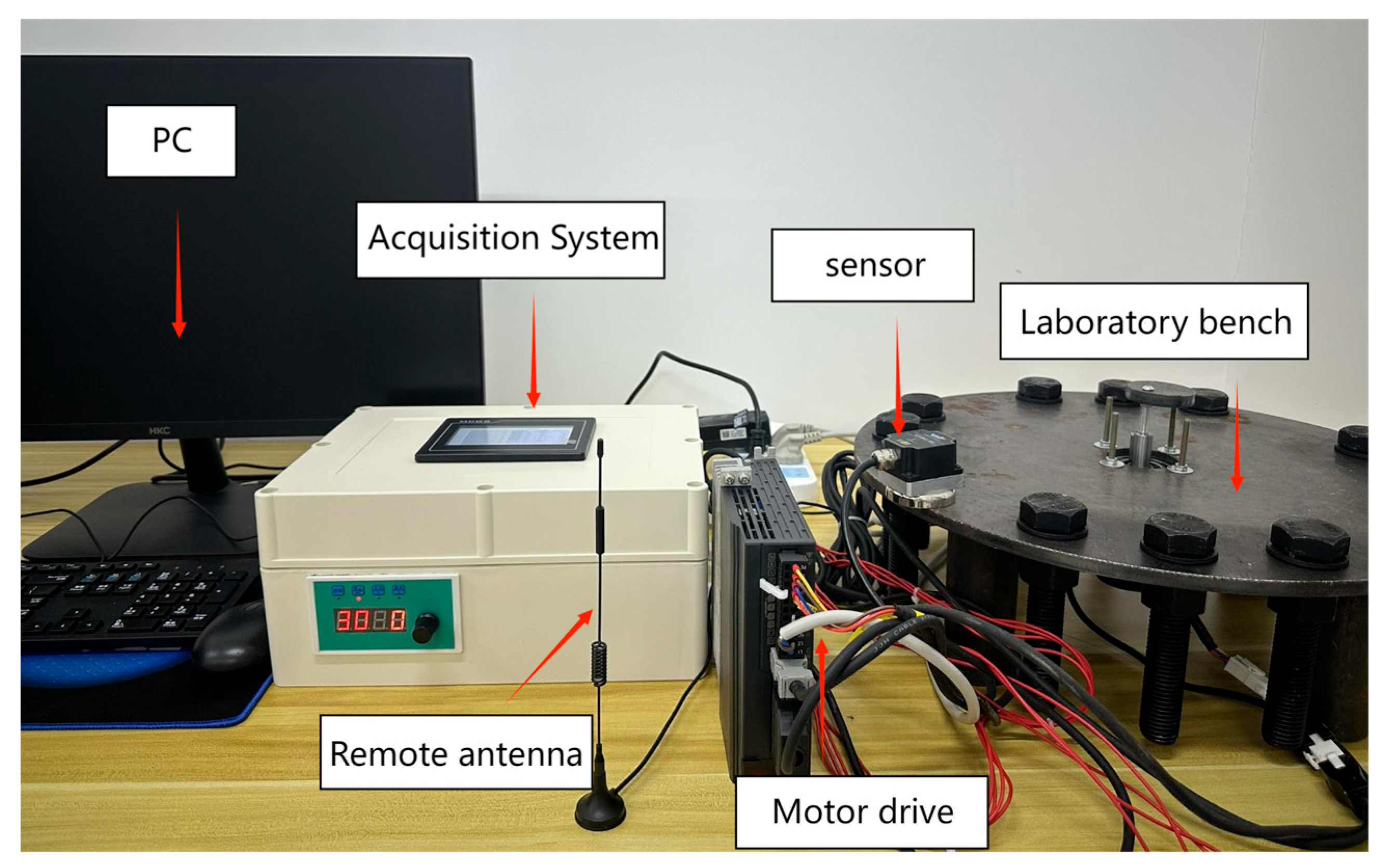
This study proposes an early detection and identification method for high-strength bolt loosening based on vibration signals combined with machine learning classifiers. The experimental setup, shown in Figure 3, includes an accelerometer, data acquisition system, signal receiver, motor driver, PC terminal, and a mechanical torque wrench to control bolt torque values. The core structure references the high-strength bolt layout of wind turbine towers: Twelve M24 high-strength bolts (labeled A–L, with specific distribution shown in Figure 4) join a Q235 steel circular plate (diameter 450 mm, thickness 9.75 mm). Four Q235 steel cylinders (dimensions: diameter 50 mm, thickness 130 mm) provide symmetrical support, simulating the bolt layout and material properties of the main shaft flange for 1.5 MW–3 MW wind turbines. The servo motor, serving as the exciter, is secured beneath the steel plate’s center using four M2×3 steel bolts. It generates periodic vibrations via an eccentric wheel. Additionally, the servo motor enables operation at speeds up to 3000 RPM. The accelerometer sensor (manufacturer: Vite Intelligent, WT-VB02-485, Beijing, China) captures mechanical structure acceleration data. The data acquisition device is equipped with a PC4023Ki touchscreen featuring a resolution of 480 × 272. It incorporates an ARM 800 MHz processor with 128 MB of memory, supporting cloud data uploading and multi-terminal management capabilities. Communication with the device is enabled via a serial port, making it suitable for industrial-grade environments. For subsequent data processing and analysis, a high-performance computer is configured. It features an AMD Ryzen 9 9950X3D processor, an RTX 5090D graphics card, a 4 TB hard drive, and G.Skill DDR5 96 GB (48 GB × 2) 6000 MHz memory. This computer delivers a robust hardware performance, efficiently supporting subsequent tasks such as training and inference of various deep learning models using Python (2025.1).

The sensor is mounted at the midpoint between bolts A and L. This location avoids the direct stress point of the bolts and resides within a structurally rigid zone, not only ensuring higher vibration signal values but also maximizing the collection of effective vibration signals. Signals are acquired at a fixed sampling rate of 16,000 times per second, with the collected data stored using MySQL Workbench 8.0 CE software. Additionally, a mechanical torque wrench can be used to control the preload magnitude of high-strength bolts, reproducing the preload decay failure observed in actual operating conditions. The vibration signals collected in the experiment align with the signal dimensions of the wind turbine SCADA monitoring system, ensuring the experimental data supports the engineering application of machine learning models.

According to the performance grade of bolts and the provisions of national standards and industry specifications, the initial torque for standard M24 × 8.8 high-strength bolts is 500 N·m, representing a healthy condition. If the torque value during retightening falls below 90% of the initial value (i.e., below 450 N·m), it must be judged as the onset of premature loosening, constituting a failure condition. The experiment employed a preset mechanical torque wrench (Manufacturer: Vite, Model: WT3-500, Accuracy: ±3%, Figure 4, range 100–500 N·m). To prevent complete bolt detachment, this study selected 500 N·m as the bolt tightening state (i.e., healthy condition) torque value and adopted the mechanical wrench’s minimum range of 450 N·m as the initial torque for early loosening (i.e., failure condition).

To collect sufficient vibration signals for early bolt-loosening detection, experimental data were acquired at two rotational speeds: 1000 RPM and 3000 RPM. This approach avoids overfitting to a single speed and enhances adaptability to speed fluctuations in practical applications.

Table 2. 3000 RMP fault classification cases.

Fault Label	Fault Location	Fault Category
0	Nothing	Heath-3000
1	A	Fault-A-3000
2	B	Fault-B-3000
3	C	Fault-C-3000
4	D	Fault-D-3000
5	E	Fault-E-3000
6	F	Fault-F-3000
7	G	Fault-G-3000
8	H	Fault-H-3000
9	I	Fault-I-3000
10	J	Fault-J-3000
11	K	Fault-K-3000
12	L	Fault-L-3000

illustrates the one-to-one mapping relationship between a single bolt failure and vibration signals at 3000 RPM, preventing localization confusion caused by signal coupling during multiple bolt loosening. The experiment collected 24 sets of fault state data and 2 sets of fully healthy state data, ultimately forming a 26-set core dataset that comprehensively supports fault diagnosis model training.

The CNN-GRU model architecture proposed by this research is shown in

Table 3. CNN-GRU model architecture parameter table.

Component	Parameter Name	Parameter Value
Input	Input dimensions	(1, 1024)
	Number of output classes	13
CNN Layer	Number of convolutional layers	5 layers
	Convolution kernel size	64 → 16 → 8 → 3 → 3
	Number of output channels	16 → 32 → 48 → 64 → 64
	Pooling method	MaxPool1d(2,2)
GRU Layer	Number of GRU layers	2 layers
	Number of hidden units	32,1
	Temporal segmentation	8 segments × 128 points
Fully Connected Layer	Network architecture	128 → 64 → 13
	Dropout rate	0.5
Activation Function	Hidden layer	ReLU
	Output layer	Softmax
Regularization	Batch normalization	CNN Layer 1

, which details the parameter configurations for each model component. These are crucial for understanding the model design logic, reproducing the model implementation, or further optimizing the model.

4. Results and Discussion

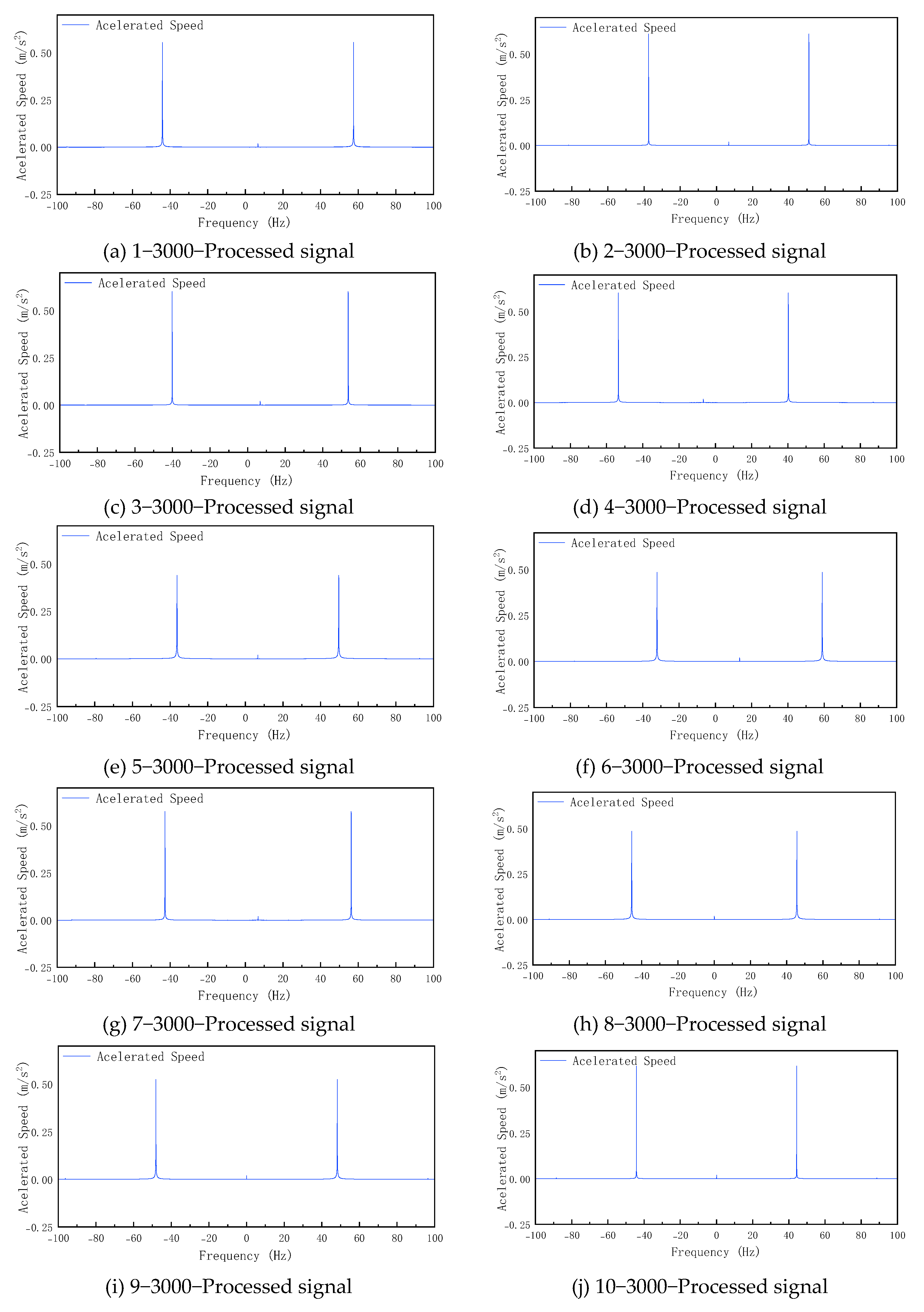
This experiment employed a sampling frequency of 16 kHz and a sampling duration of 10 s, with 120 test sets conducted for each fault category to increase the sample size. After connecting the sensors and initiating the acquisition system, the AC servo motor was activated. Detection ceased upon completion of sampling. The acquired signals underwent preprocessing using the Fast Fourier Transform (FFT) algorithm, yielding visualized vibration signal plots for different fault categories. Figure 5 and Figure 6, respectively, show the preprocessing and postprocessing signal visualizations for labels 1 to 12 under operating conditions of 3000 revolutions per minute.

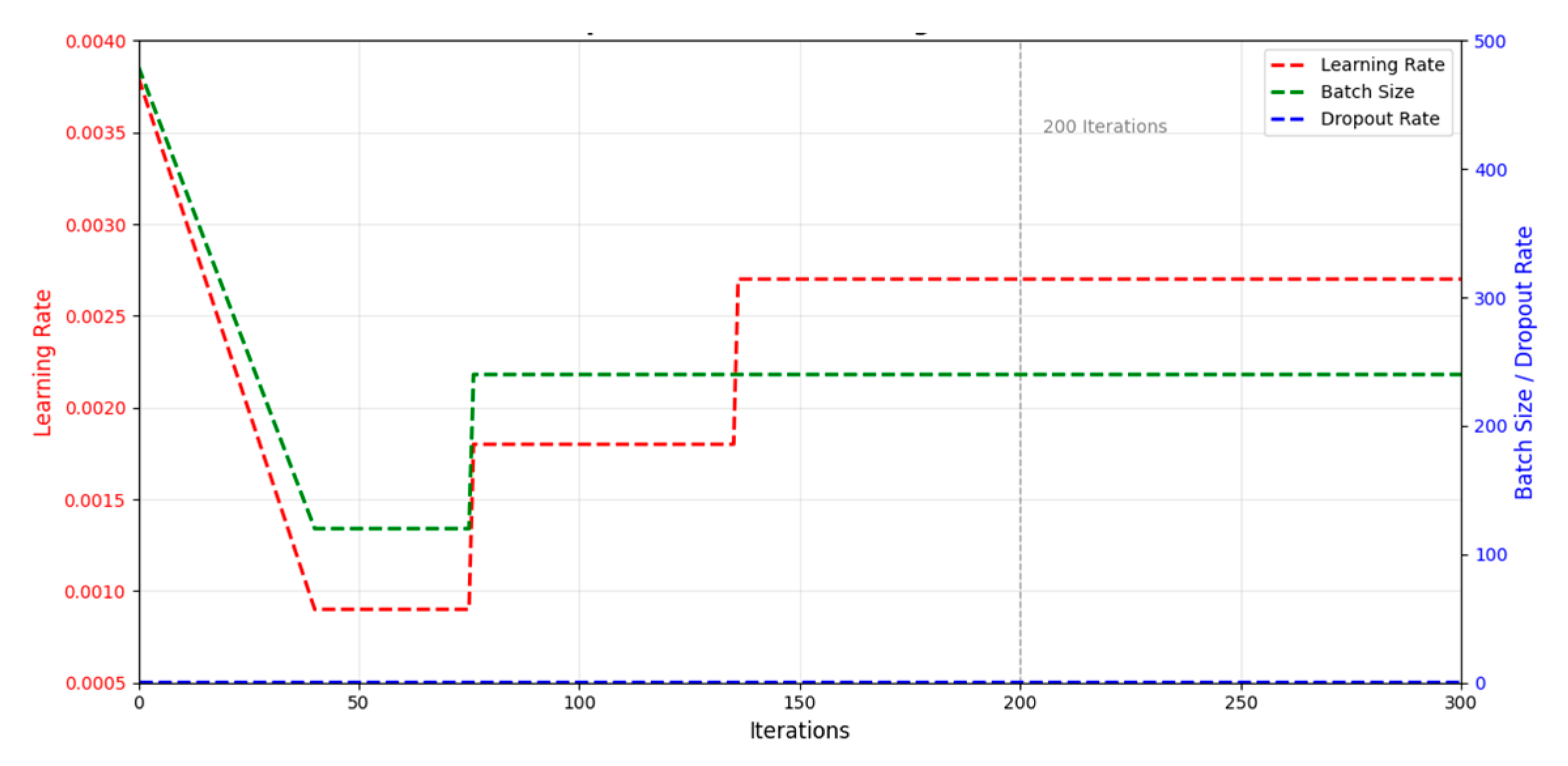
By optimizing the CNN-GRU model using BKA, we specified search ranges for each parameter in Table 1 with a maximum iteration count of 300. The iteration process is illustrated in Figure 7. After 300 iterations, the fitness value stabilized. At this point, the batch size was 240, the learning rate was 0.0027, and the dropout rate was 0.5.

The optimal solution from

Table 4. Optimal parameters obtained by BKA optimization.

Name	Scope	Value
batch_size	[32, 512]	240
learning_rate	[1 × 10−4, 1 × 10−2]	0.0027
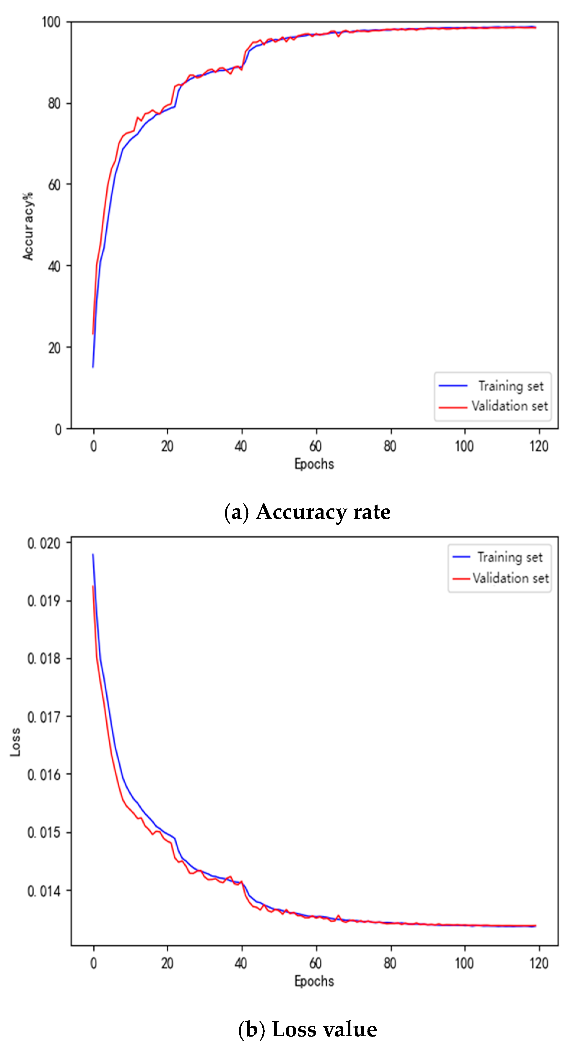
dropout_rate	[0.1, 0.9]	0.5

is used to update the corresponding hyperparameter values in the original model, yielding the BKA-CNN-GRU model. This model is then retrained using the training dataset. As shown in Figure 8, both training and validation accuracy converge rapidly with increasing iterations: both surpass 80% within the first 20 iterations and approach 100% after 40 iterations, maintaining long-term convergence. This indicates strong learning generalization for temporal–spatial fault features without overfitting. Simultaneously, the training and validation loss curves on the loss curve rapidly decrease in tandem and ultimately converge stably, with good consistency between the training and validation loss curves.

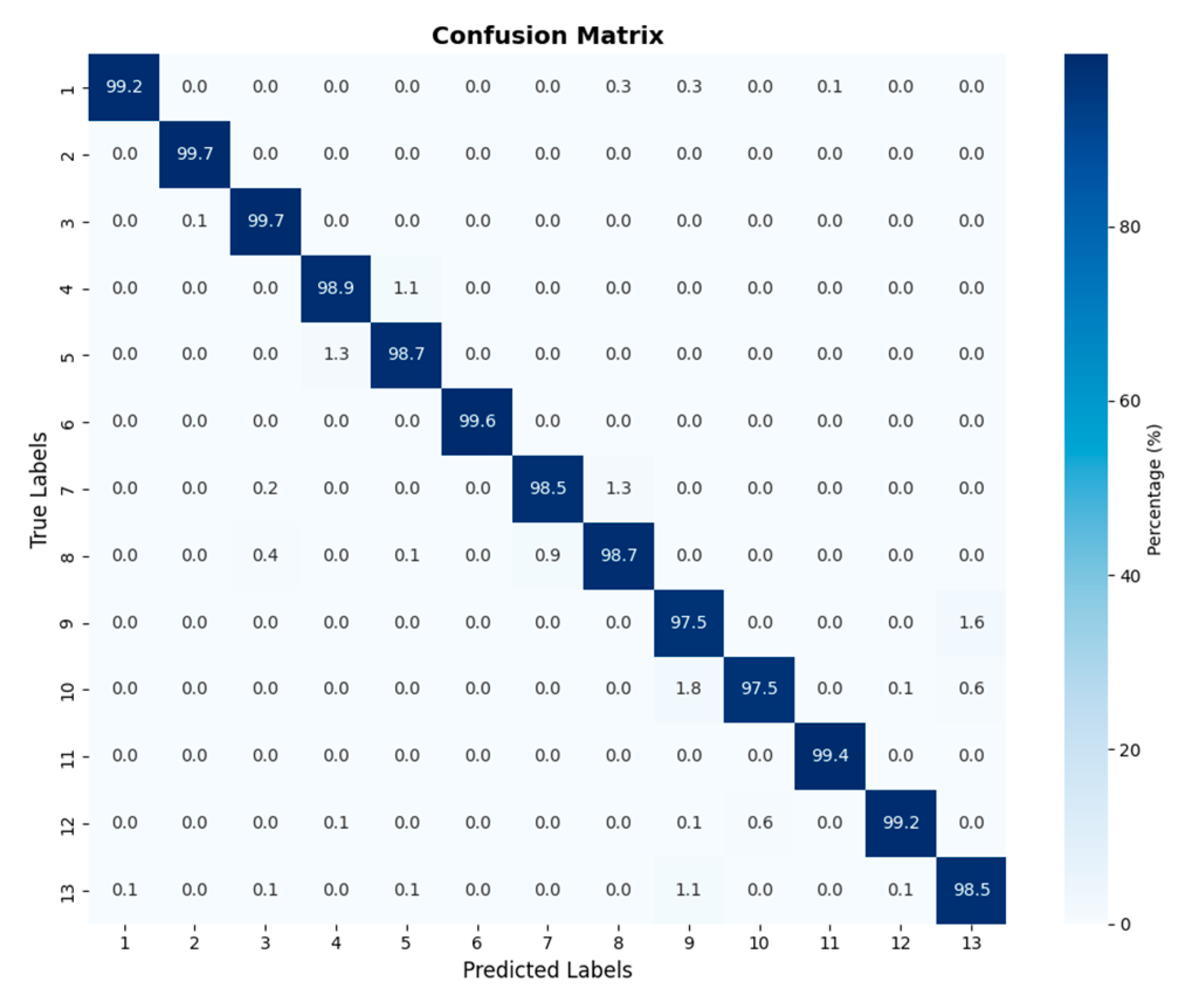
Figure 9 presents the confusion matrix results of the proposed model for detecting high-strength bolt-loosening faults. Also known as an error matrix, the confusion matrix serves as a crucial metric for evaluating classification accuracy. It not only analyzes and highlights issues in the data classification process but also carries explicit structural meaning: each row corresponds to the true labels of the data, while each column corresponds to the model’s predicted labels. This confusion matrix demonstrates the BKA-CNN-GRU model’s outstanding classification performance across 13 fault categories. Over half of the categories achieve a prediction accuracy of 98%, while the remaining categories maintain an accuracy above 97.5%. Only a very small number of categories exhibit an extremely low proportion of misclassifications. Overall misclassification is minimal, indicating the model’s ability to accurately distinguish between different fault types.

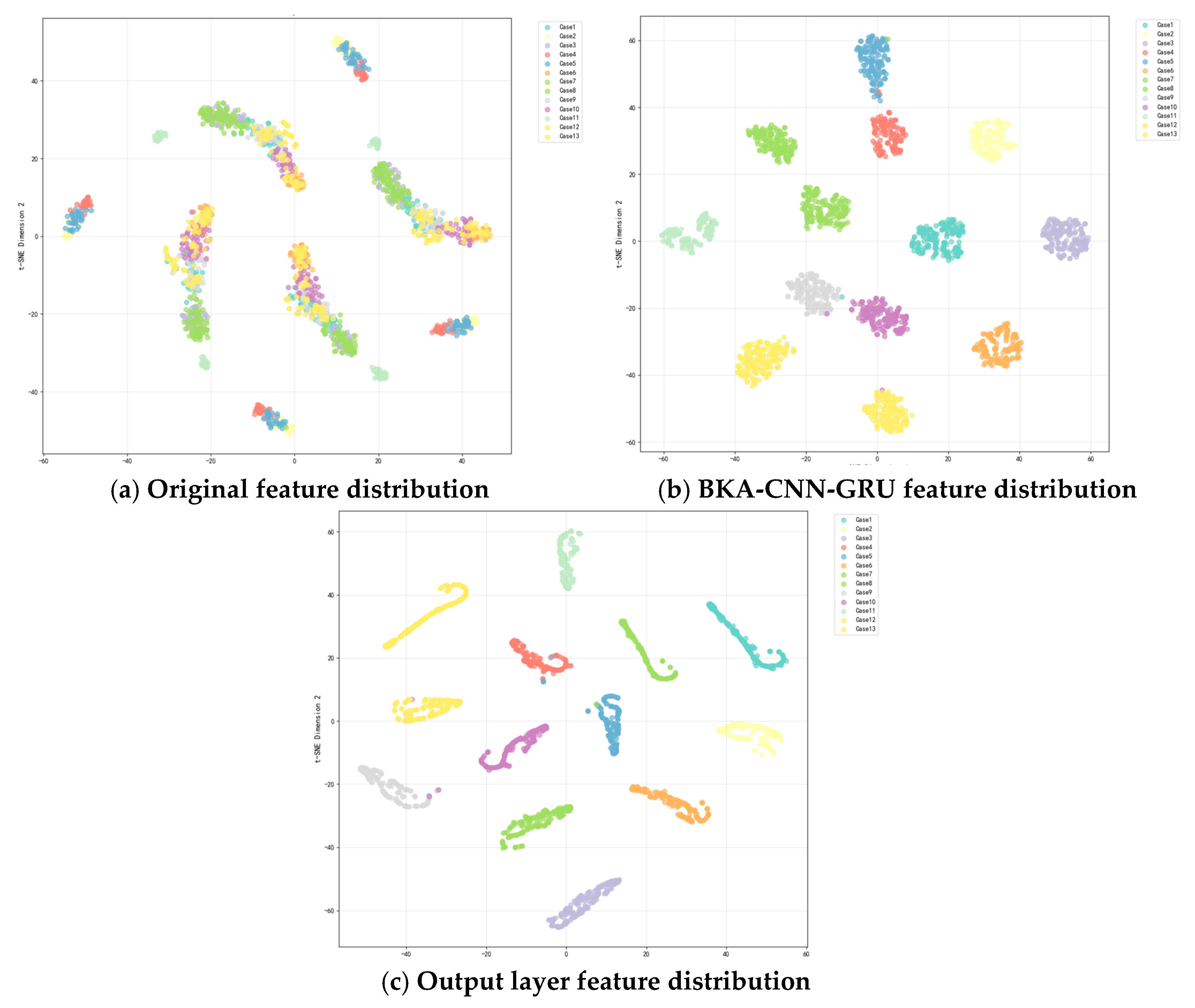
t-SNE (t-distributed Stochastic Neighbor Embedding) is a nonlinear dimensionality reduction algorithm primarily used for high-dimensional data visualization. It achieves this by mapping similarity in high-dimensional space to a lower dimension, causing similar data points to cluster together while separating dissimilar ones. This effectively preserves local data structures and reveals group distribution characteristics. To further validate the effectiveness of feature extraction by the BKA-CNN-GRU model, the features from its final fully connected layer underwent t-SNE dimensionality reduction, as shown in Figure 10.

As shown in Figure 10, the original features exhibit scattered and overlapping points across different categories, with a blurred clustering structure and indistinct boundaries between categories. After CNN convolution operations and GRU temporal processing, the point distributions for different fault types become clearly defined, and the boundaries between categories are improved. Notably, the separability of edge categories is significantly enhanced, indicating that the network has extracted richer category features. Finally, after passing through the fully connected layer and Softmax normalization module, the feature distribution becomes tightly clustered and completely separated. All categories form distinct clusters, demonstrating the network’s successful extraction of multi-level and dynamic features. Feature points for each category form compact, mutually exclusive clusters with clear boundaries. This achieves an excellent classification performance, significantly enhancing the distinguishability between different feature categories and validating the model’s effectiveness in feature extraction.

Table 5. Comparison of model diagnostic results.

Name	BKA-CNN-GRU	CNN-GRU	SwinTransformer+SENet
Training set accuracy/%	99.75	98.41	86.99
Verify set accuracy/%	98.86	96.53	87.56
Average accuracy/%	99.31	97.47	87.28
Time/s	6.04	20.23	24.25

presents a comparative analysis of diagnostic results across four models: BKA-CNN-GRU, CNN-GRU, and SwinTransformer+SENet [66]. Using the same dataset, each model was evaluated based on four dimensions: training set accuracy, validation set accuracy, average accuracy, and inference time. It can be observed that the BKA-CNN-GRU model achieves 99.75% accuracy on the training set, validation set, and average accuracy, significantly outperforming the other models. Additionally, this model demonstrates superior efficiency, with an average processing time of only 6.04 s per iteration. Overall, the BKA-CNN-GRU model demonstrates a superior performance in diagnostic tasks by combining higher accuracy with enhanced computational efficiency.

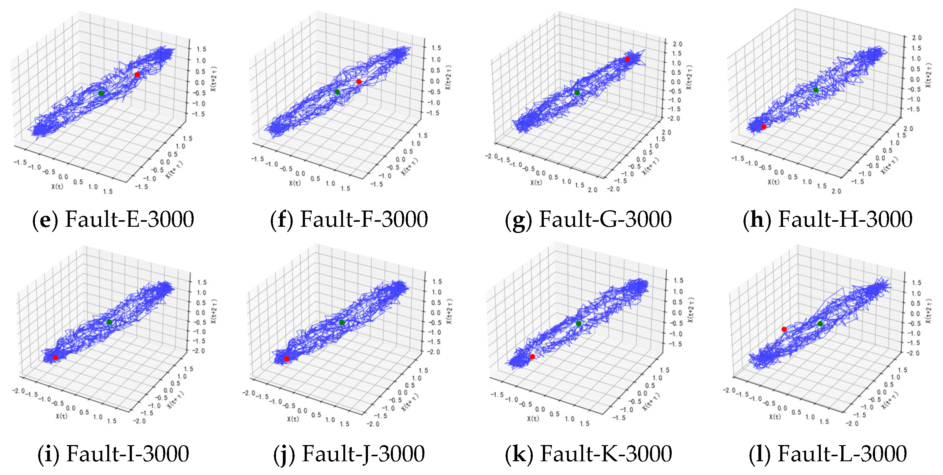
Additionally, to validate the compatibility of the proposed model, it was integrated with chaos theory to analyze nonlinear feature information. Through phase space reconstruction techniques, time-domain signals were mapped into high-dimensional space to examine their chaotic characteristics. Diagnostic analysis was performed using the same dataset employed in the experiments. To illustrate chaotic states across different fault categories, two-dimensional chaotic phase diagrams labeled for classes 1–12 are presented in Figure 11. As shown in Figure 11, the chaotic phase diagrams for each state exhibit distinct complex patterns. While they share an overall distribution resembling a fuzzy ball, each state’s diagram differs in density, edge structure, and symmetry. This reflects the distinct evolutionary patterns of fault signals within chaotic attractors.

As shown in

Table 6. Effect of different signal processing methods on model diagnostic accuracy.

Signal Processing Methods	Accuracy Rate%
Fast Fourier Transform	99.32
Chaos Principle	98.86

, the recognition rate achieved by applying the chaotic principle processing in conjunction with the BKA-CNN-GRU model reached as high as 99.32%. Compared to applying the Fast Fourier Transform (FFT) to the signal, both approaches demonstrated high overall accuracy levels. This also indicates that the core fault feature in this diagnostic scenario is periodic frequency anomalies. This scenario aligns highly well with the frequency-domain analysis capabilities of FFT, while the nonlinear features extracted by the chaos principle are only marginally inferior to frequency-domain features in terms of feature discriminative power.

Comparative analysis with other models demonstrates that the proposed model exhibits outstanding accuracy in high-strength bolt fault diagnosis, while also presenting certain limitations. Specifically, first, its small-sample learning capability is remarkable. The BKA-CNN-GRU model performs exceptionally well with limited data samples. The global search capability of the BKA optimization algorithm effectively prevents overfitting, while the CNN-GRU fusion architecture enables effective feature learning using limited training data. Additionally, the model integrates multiple components—BKA optimization, CNN-GRU networks, and data preprocessing—requiring simultaneous adjustment of multi-level parameters, which may impact algorithm stability and reproducibility. Second, it demonstrates significant advantages in frequency-domain feature extraction. Comparing FFT transformation and chaos theory preprocessing methods validates the effectiveness of FFT preprocessing in bolt-loosening fault identification. FFT enhances signal frequency-domain characteristics. Combined with the time-frequency joint analysis capability of CNN-GRU, it extracts more discriminative feature representations, significantly improving fault recognition accuracy. However, the advantage of FFT preprocessing is scenario-dependent, primarily suitable for analyzing stationary signals. For non-stationary or transient fault signals, it may fail to fully capture dynamic characteristics. Third, computational efficiency and accuracy are balanced. Compared to complex models like SwinTransformer+SENet, the proposed method achieves lower computational complexity while maintaining high accuracy. FFT preprocessing incurs minimal computational overhead, making the overall architecture suitable for real-time monitoring applications. However, the BKA optimization strategy, designed for specific data characteristics, may have limited generalization capabilities. The current comparative experiments have limited coverage and require further validation against more advanced methods.

The postprocessing model can be effectively applied to engineering practice through three key approaches: In data processing, select appropriate sensors and installation locations based on actual operating conditions. For instance, first identify vibration-sensitive areas of bolts or damage-prone zones in specific mechanical structures, then install sensors at these critical points to collect high-intensity vibration data, providing high-quality data support. For model optimization and adjustment, retrain and fine-tune the model using additional real-world failure data to enhance its accuracy in identifying complex failures and improve generalization capabilities. Simultaneously, explore integrating non-destructive testing sensors to build a multi-parameter diagnostic system, enabling precise diagnosis of diverse bolt failure modes. At the system integration level, integrate the model into the wind turbine tower bolt condition monitoring platform for real-time diagnostics. Simultaneously explore deep integration with life analysis by incorporating life analysis methodologies. This involves using fault diagnosis results as dynamic prior information to continuously update the life prediction model, achieving a unified dynamic mapping of fault characteristics, degradation rates, and remaining useful life (RUL).

5. Conclusions

This paper proposes a high-strength bolt-loosening fault diagnosis framework integrating Fast Fourier Transform (FFT) feature extraction with a BKA-CNN-GRU collaborative mechanism: raw data undergoes FFT preprocessing, combined with a BKA-optimized CNN-GRU model for fault identification. Experimental validation demonstrates its significant advantages, with specific conclusions as follows:

(1)

The diagnostic features constructed by combining FFT with window functions and power spectrum estimation effectively address the difficulty of identifying periodic fault characteristics through single-time-domain analysis while reducing the computational complexity of traditional Fourier Transforms.

(2)

The CNN-GRU fusion architecture leverages the strengths of both components: the CNN extracts local impact features from vibration signals via its local receptive field and weight sharing, while the GRU models long-term temporal dependencies through gating mechanisms to overcome the vanishing gradient problem in traditional RNNs. Furthermore, the CNN’s dimensionality reduction capability alleviates the GRU computational burden, compensating for the feature extraction limitations of either model alone.

(3)

Under identical datasets and feature dimensions, BKA’s adaptive optimization enhances both the accuracy of the CNN in extracting local impact features and the capability of the GRU in capturing temporal evolution patterns, enabling the model to identify fault features with higher distinguishability.

Experiments demonstrate the model’s outstanding fault recognition accuracy, providing an innovative solution for detecting high-strength bolt loosening in large-scale equipment like wind turbines. It is particularly suitable for early-stage loosening detection, effectively preventing fault escalation and enhancing operational safety.