Abstract
Accurate prediction of CO2 corrosion under dense-phase and supercritical conditions remains a critical challenge for oil and gas pipeline integrity management. While machine learning (ML) has been applied in this field, prevailing models like the Multilayer Perceptron (MLP) often struggle to capture the complex, non-linear interactions between multiple environmental parameters, limiting their predictive accuracy and robustness. To bridge this gap, this study innovatively introduces the Kolmogorov–Arnold Network (KAN) algorithm for CO2 corrosion rate prediction. Utilizing a unique dataset of field-collected parameters (including dissolved O2, H2S, SO2 concentrations, and water cut), we developed a KAN model and conducted systematic hyperparameter optimization. Our investigation revealed the optimal network configuration (3 layers, grid = 3) and, counterintuitively, that the steps parameter does not correlate positively with performance. Most significantly, comparative experiments demonstrated that the KAN model substantially outperforms traditional MLP, achieving superior prediction accuracy alongside faster computational speed and lower loss values. These findings not only provide a robust tool for precise corrosion prevention in oilfield operations but also highlight the potential of KAN as a novel, efficient, and highly accurate framework for tackling complex problems in materials degradation.
1. Introduction
CO2 corrosion is a critical issue in the oil and gas industry, particularly in metal facilities such as drilling equipment, casing, and surface pipelines. The corrosion mechanism is primarily related to the dissolution of CO2 in water [1,2]. When CO2 dissolves in water, it forms carbonic acid (H2CO3), which reacts with the metal surface in an acidic environment to produce corrosion products such as iron carbonates. Meanwhile, the hydrogen ions (H+) released during the reaction further accelerate the dissolution of the metal. The corrosion rate of CO2 is influenced by various factors, including CO2 concentration, temperature, pH, flow rate, and other parameters. Additionally, the presence of corrosive components such as hydrogen sulfide and chloride ions exacerbate the corrosion process, making CO2 corrosion highly complex and uncertain [3,4]. It should be emphasized that under certain high-pressure and high-temperature conditions, CO2 enters a dense phase and may become supercritical (critical point: 31.1 °C, 7.38 MPa). In this state, the physical and chemical properties of CO2, such as density, solubility, and mass transfer behavior, differ significantly from those of gaseous or liquid CO2 [5,6]. Consequently, corrosion mechanisms under supercritical CO2 environments cannot be simply equated with those in conventional pipelines [7,8]. This distinction is crucial to avoid misunderstanding that the current study targets general oil and gas pipeline conditions, while in fact it is focused on dense-phase CO2 systems. The hazards of this corrosion are severe. In addition to accelerating equipment aging and increasing maintenance costs, it can lead to pipeline leaks, equipment failure, and even more serious safety incidents. Therefore, accurately predicting and preventing CO2 corrosion has become an urgent engineering challenge in the oil and gas industry. To effectively address this challenge, precise prediction tools and protective measures are needed to ensure the safe operation and reliability of equipment, thereby reducing the potential risks and economic losses caused by corrosion [9,10,11,12].
Traditional methods for predicting CO2 corrosion rates are primarily categorized into empirical models (e.g., De Waard-Milliams, Norsok M, Nesic, and Jepson formulas [13,14], semi-empirical models (e.g., DWM model, De Waard 93 model, and resistance model [15,16,17,18,19,20,21], and first-principle (mechanistic) models based on electrochemical and transport theory [22]. While empirical and semi-empirical models offer practical solutions within specific parameter ranges by combining experimental data with correlative or partial mechanistic approaches, they often struggle with accuracy and generality in complex, multi-variable environments involving multiphase flow, complex fluids, and dynamic conditions. First-principle models provide deeper physicochemical insights but are typically constrained by their computational demands and need for precise input parameters that are seldom available in real-field applications. Common limitations across these traditional methods include difficulties in capturing complex non-linear interactions, fully accounting for the inhibitory effect of corrosion product films (e.g., FeCO3), and adapting to high-temperature, high-pressure, and dynamically changing environments. These challenges highlight the need for more robust and intelligent predictive methods, motivating the application of machine learning techniques like the Kolmogorov–Arnold Network (KAN) in this study to improve prediction reliability by directly learning from data without pre-defined mechanistic assumptions.
In recent years, with the advancement of data science and artificial intelligence, the application of machine learning in corrosion prediction has gained increasing attention. By analyzing large volumes of historical data, machine learning algorithms can identify underlying patterns and relationships among variables in the corrosion process, offering significant advantages in predicting complex corrosion behaviors. Machine learning models not only adapt to changes in various corrosion-influencing factors but also effectively handle nonlinear and high-dimensional data, providing scientific support for addressing the diversity of corrosion environments. Additionally, machine learning methods enable continuous improvement in prediction accuracy and stability through adaptive model optimization, making them suitable for various industrial corrosion scenarios. As industrial environments become more complex and corrosion challenges intensify, machine learning technology demonstrates broad application potential and promising prospects in corrosion prediction.
CO2 corrosion prediction is often automated or semi-automated using computer algorithms, such as clustering and supervised learning methods. To enable automated prediction of CO2 corrosion in steel pipes, researchers have developed various algorithms and techniques. Machine learning methods are generally divided into classification and regression based on task type, with regression mainly used to predict corrosion rate as a continuous variable. By leveraging machine learning, algorithms can automatically extract features from large datasets and generate predictive models, effectively improving the accuracy and efficiency of corrosion prediction, ensuring robust applicability even in complex environments. Various supervised learning algorithms have been widely applied to predict carbon dioxide corrosion rates, including Random Forest (RF), Support Vector Machine (SVR), Gradient Boosting Decision Tree (GBDT), K-Nearest Neighbors (KNN), and Multilayer Perceptron (MLP) [23,24,25,26,27,28,29,30]. While these methods represent a significant advance over traditional models, each carries inherent limitations. For instance, tree-based ensembles like RF and GBDT can capture non-linearities but often struggle to extrapolate beyond their training data. SVR models are sensitive to kernel choice and hyperparameter tuning, and their results can be difficult to interpret physically. A more fundamental challenge common to many ML approaches, including the widely used MLP, is their lack of interpretability. They often function as ‘black boxes’, offering limited insights into the relative importance of input variables or the underlying mechanistic relationships.
This lack of interpretability, combined with their potential inefficiency in learning highly complex functions, becomes a critical bottleneck when applying ML to unprecedented challenges such as predicting corrosion in dense-phase and supercritical CO2 systems. The extreme conditions and complex, non-linear interdependencies among parameters (e.g., H2S, SO2, water cut under high pressure/temperature) demand models that are not only accurate but also transparent and efficient. Thus, there is a pressing need for a novel modeling approach that can address these dual requirements of high accuracy and operational interpretability.
To address these limitations, this study pioneers the application of the novel Kolmogorov–Arnold Network (KAN) for predicting corrosion rates in dense-phase/supercritical CO2 environments. We hypothesize that KAN’s unique architecture, which learns adaptive activation functions along edges rather than fixed neuronal activation, grants it superior capability to capture the intricate non-linearities and interaction effects inherent in our specialized field dataset (sourced from 43 research articles, encompassing key variables like Cr, Temp, H2O, O2, H2S, SO2). The primary objectives of this work are threefold: (1) To develop and systematically optimize a KAN model for this specific prediction task, elucidating the impact of key hyperparameters (Steps, Layers, Grid); (2) To conduct a rigorous comparative performance evaluation against a well-established MLP benchmark, quantifying improvements not only in predictive accuracy but also in computational efficiency; and (3) To leverage KAN’s purported interpretability to explore and rank the influence of input features, thereby transcending mere prediction and offering potential insights into the corrosion process itself.
The remainder of this paper is structured as follows: Section 2 elucidates the methodological framework, including the theoretical foundations of the Kolmogorov-Arnold Network (KAN) and Multilayer Perceptron (MLP) architec-tures, along with the experimental design for parameter sensitivity analysis. Section 3 describes the dataset charac-teristics and presents comprehensive correlation analysis. Section 4 provides detailed experimental results and dis-cussion, focusing on hyperparameter optimization effects and comparative performance between KAN and MLP models. Finally, Section 5 concludes with principal findings and their implications.
2. Methods
2.1. Introduction of the Kolmogorov–Arnold Network (KAN)
The Kolmogorov–Arnold Network (KAN) is a neural network model based on the Kolmogorov–Arnold theorem, capable of representing complex multivariate continuous functions [31]. Unlike traditional MLPs, the outputs of KAN nodes are not directly subjected to standard nonlinear activations (Figure 1).
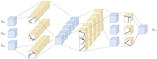
Figure 1.
The network diagram of the KAN architecture.
The mapping from input to output in KAN follows the standard KAN formulation [31], where each layer computes a combination of univariate functions to approximate complex multivariate relationships.
In the formula, x represents the input, n is the number of input variables in x, is the basic univariate function, and denotes the inner sum. is the result of the inner sum, which acts as the input function for the outer tier. Thus, the entire function f(x) is the sum of the sub-functions .
Usually, the basis function is set to the SILU function, which is
SILU is a neural network activation function, also known as the Swish function. It achieves nonlinear transformation by multiplying the input with the output of the sigmoid function. In most cases, the spline function spline(x) is parameterized as a linear combination of B-splines, represented as
The B-spline component allows the activation functions to capture subtle nonlinear patterns, enhancing the model’s flexibility. Cubic splines can capture subtle variations in the data while ensuring smoothness of the curve, and they are computationally efficient, making them suitable for use in deep learning models.
2.2. MLP (Multilayer Perceptron)
A standard Multilayer Perceptron (MLP) was employed as a baseline model. The network consists of an input layer, multiple hidden layers, and an output layer (Figure 2), with ReLU activation functions introducing nonlinearity.
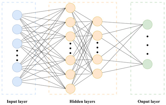
Figure 2.
Multilayer Perceptron Network structure diagram.
The input layer is responsible for receiving the input information of the network model, usually taking the feature vectors of data samples as the input information. After further processing through multiple hidden layers and the output layer, the output layer provides the experimental results [32]. The number of nodes and layers in the hidden layers can be adjusted according to the specific needs of the experiment. The MLP learns to map input information to output results. To enhance the accuracy of model predictions, the corresponding parameter weights and bias values are continuously updated and adjusted during model training. Activation functions are typically added between layers to introduce non-linear factors.
In this context, represents the input data, represents the weight, represents the threshold, represents the output, and f represents the activation function. Activation functions introduce non-linearity, allowing MLPs to learn and represent more complex features and patterns. This enables the mapping of complex non-linear functions between inputs and outputs. In the network, activation functions are responsible for mapping the inputs of neurons to the outputs. Common activation functions include ReLU, Sigmoid, and Tanh. ReLU is the most commonly used activation function today due to its simplicity and efficiency, making it suitable for deep networks. Sigmoid and Tanh are used in specific scenarios, such as probability predictions and situations where outputs need to be centered around zero, but they suffer from the vanishing gradient problem.
MLPs typically require multiple rounds of training, each involving forward propagation and backward propagation, combined with gradient descent to adjust the parameters. In forward propagation, the output of neurons from the previous layer is used as the input for the next layer, calculating the output until the information reaches the output layer. Let l denote the layer number in the neural network, represent the output of the -th layer, and denote the weights and biases between the (−1)-th and l-th layers, and be the activation function of the -th layer. The forward propagation process can be expressed as
The weights are the parameters that need to be learned. The neural network continuously adjusts these parameters to minimize the loss function, which measures the difference between the network’s predicted values and the actual values. For regression problems, the mean squared error is typically chosen as the loss function:
where y is the actual value of the neural network output, y′ is the predicted value of the neural network, No is the number of neurons in the output layer, and β is a hyperparameter that balances the contribution of the L2 regularization term and the standard objective function.
2.3. Parameter Sensitivity Analysis and Experimental Design
To systematically investigate the influence of key architectural and training hyperparameters on the performance of Kolmogorov–Arnold Networks (KAN), a comprehensive parameter sensitivity analysis was conducted. The objective was to determine the optimal configuration that balances predictive accuracy, generalization capability, and computational efficiency. The experiments were designed to isolate and evaluate the effects of the number of hidden layers, the grid density of the spline functions, and the number of training steps.
The following hyperparameters and their respective value ranges were defined for the study:
- ➀
- Number of Hidden Layers: The depth of the network was varied across {1, 2, 3, 4} layers. The number of neurons per hidden layer was held constant for a given experimental series.
- ➁
- Grid Size (grid_size): The number of grid points used to define the spline functions was tested across a range of {1, 2, 3, 4, 5}. This parameter directly controls the expressivity and complexity of the spline approximations.
- ➂
- Number of steps (steps): The number of gradient descent updates per training session was evaluated for values of {5, 10, 15, 20}. This parameter influences both the convergence behavior and the computational cost.
For each unique combination of hyperparameters within the defined search space, an independent KAN model was instantiated and trained. To ensure a fair and controlled comparison, the following parameters were kept constant across all experiments unless otherwise specified: the L1 regularization coefficient (lamb = 0.01), the entropy regularization coefficient (lamb_entropy = 2), the optimizer settings, and the initial learning rate. All models were trained and evaluated on identical, fixed training, validation, and test splits of the dataset.
Model performance was quantified using three primary metrics: the value of the Loss function (specifically, Mean Squared Error, MSE), the Mean Squared Error (MSE) itself, and the Coefficient of Determination (R2). The MSE calculates the average of the squared differences between predicted and observed values, while the R2 metric assesses the proportion of variance in the target variable that is predictable from the input features. To ensure statistical robustness and account for variability in random initialization, each hyperparameter configuration was trained and evaluated across n = 3 independent runs with different random seeds. The final reported results for each configuration represent the mean and standard deviation of these runs. The optimal model was selected based on its performance on a held-out validation set, prioritizing the highest R2 value.
In addition to predictive accuracy, the computational cost incurred during training and inference for each hyperparameter configuration was recorded. The total wall-clock time was measured to analyze the trade-offs between model performance (Loss, MSE, R2) and runtime efficiency as a function of network depth, grid size, and number of steps.
3. Data Description and Analysis
Machine learning algorithms fall into two main categories: supervised learning and unsupervised learning. Supervised learning involves training a model on labeled data, where both the input data and their corresponding labels are known, and then mapping new input data to these labels [33]. This category includes classification and regression tasks. Classification deals with predicting discrete outcomes, such as using X-ray imaging to detect and categorize tumors as either present or absent. Regression, in contrast, focuses on predicting continuous values, like forecasting future stock prices based on historical data and other relevant features. Unsupervised learning, however, involves identifying patterns and relationships within the data without predefined labels [34]. For instance, it can segment customers into distinct groups based on their shopping behaviors, aiding in the development of targeted marketing strategies. In the context of predicting corrosion rates, machine learning methods predominantly use supervised learning algorithms.
The machine learning workflow involves: (1) preparing the dataset, (2) partitioning the data into training and evaluation subsets—randomly splitting the dataset into a training set and a test set, with 80% of the data used for training and 20% for testing, and applying 5-fold cross-validation on the training set to ensure robust model evaluation, (3) training multiple models with the prepared dataset, and (4) assessing the performance of these models using the evaluation subset. The complete process is depicted in Figure 3.
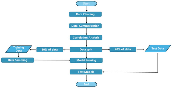
Figure 3.
The flowchart of the machine learning model used in this study.
3.1. Data Summary
The data is derived from the article “Update of DNV Recommended Practice RP-J202 with Focus on CO2 Corrosion with Impurities” [8], as well as from articles such as “Understanding the influence of SO2 and O2 on the corrosion of carbon steel in water-saturated supercritical CO2”, and others [35,36,37]. In total, there are 248 sample data points, encompassing ten features including material, chromium content, temperature, pressure, etc. The output includes corrosion rates along with their respective corrosion grades. Table 1 provides statistical information on the influencing factors’ data. The dataset was compiled from four peer-reviewed journal articles and a recommended practice issued by DNV (RP-J202), all focusing on CO2 corrosion mechanisms in carbon steel under different impurity levels. These sources were selected because they provide quantitative experimental data on corrosion rates and related parameters, with clear descriptions of testing environments and materials.

Table 1.
Data Summary.
The final dataset consists of 248 experimental observations collected from four peer-reviewed studies and one recommended practice issued by DNV, all investigating CO2 corrosion of carbon steel with impurities. For each observation, ten input variables were recorded, including material type, chromium content, temperature (°C), pressure, and concentrations of SO2, O2 and other impurities (ppmv), as well as exposure time (h). The target variables are the corrosion rate (CR, mm/year) and an associated severity grade (0–3).
Descriptive statistics of the target variables are presented in Table 1. The mean corrosion rate is 0.50 mm/year, ranging from 0.00 to 26.00 mm/year, while the severity grade has an average of 2.14 and a standard deviation of 1.17, with a median value of 1. These values indicate that although many cases show low corrosion levels, some measurements reveal very high rates requiring stricter control. The dataset therefore covers a broad spectrum of conditions, providing a solid basis for modelling and trend analysis.
3.2. Correlation Analysis
Data mining involves multivariate analysis, considering not only the impact of individual factors but also studying the correlations between varied factors and the extent of each feature’s influence on the corrosion rate. Common correlation analysis methods include the Pearson correlation coefficient and Spearman correlation coefficient [38]. This study employs the Pearson correlation coefficient proposed by Karl Pearson in the 1880s to evaluate the degree of correlation between two variables X and Y. The mathematical expression is as follows:
The term Cov(X, Y) in the formula denotes the covariance between X and Y. The correlation coefficient values range from −1 to 1. A coefficient of 0 indicates that the two factors are independent of each other, with no mutual influence. A positive correlation is indicated by values between 0 and 1, where a coefficient of 1 indicates a perfect positive relationship, meaning that any increase in one variable leads to an equal increase in the other. Conversely, a coefficient between −1 and 0 represents a negative relationship, where an increase in one variable corresponds to a decrease in the other. The closer the correlation coefficient is to either −1 or 1, the stronger the correlation between the two factors.
Based on this principle, the correlation coefficients calculated for various corrosion factors can be used to generate a heat map of the correlation matrix, as shown in Figure 4.
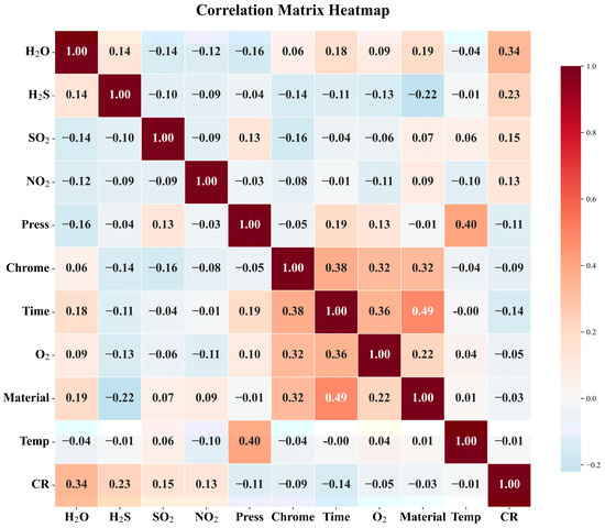
Figure 4.
Correlation matrix heatmap.
Figure 4 presents a correlation heatmap matrix illustrating the pairwise Pearson correlation coefficients among key factors influencing CO2 corrosion. The color intensity and numerical values within each cell reflect the strength and direction of the linear relationships between variables, ranging from −1 to 1. Notably, parameters such as temperature (Temp), partial pressure of CO2(Pt), and concentration of H2S exhibit varying degrees of correlation with the corrosion rate (CR), while other factors including time and material composition show comparatively weaker associations. This analysis provides critical insight into multicollinearity among predictors, thereby informing feature selection for subsequent modeling efforts and enhancing the interpretability and robustness of the predictive algorithm.
Figure 5 demonstrates the effect of different factors on the corrosion rate. The data reveal that water has the most substantial impact on the corrosion rate, with a value of 0.34, followed by hydrogen sulfide and sulfur dioxide, while temperature has a relatively minor effect. This is mainly due to water acting as a medium in the corrosion process, increasing conductivity and enhancing electrochemical reactions, thereby exacerbating the corrosion rate. Hydrogen sulfide and sulfur dioxide chemically react with the metal surface, forming sulfide protective films, which in turn affect the corrosion rate.
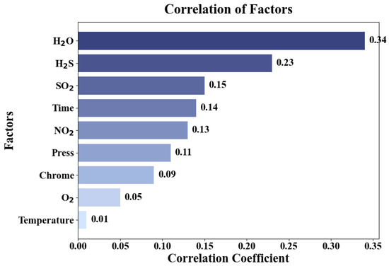
Figure 5.
The degree of influence of each factor on the corrosion rate.
4. Results and Discussion
Leveraging the insights into key features and their correlations from Section 3, this section presents the results of our predictive modeling. We conduct a systematic comparison of five distinct algorithms: the proposed KAN, traditional MLP, SVR, RF, and XGBoost. We first describe the optimization of the KAN’s hyperparameters. Then, we compare the final performance of all tuned models on a held-out test set, demonstrating KAN’s superior capability in capturing the intricate patterns inherent in the corrosion data.
4.1. Hyperparameter Optimization Analysis
By analyzing these metrics under different experimental configurations, we aim to find the optimal combination of KAN network structure and parameters to enhance the model’s prediction accuracy and generalization capability.
4.1.1. The Impact of the Number of Hidden Layers on Model Performance
To investigate the impact of the number of hidden layers on the performance of KAN models, we designed a series of experiments. The experiments were conducted by setting the same number of neurons but varying the number of hidden layers (1 layer, 2 layers, 3 layers, and 4 layers), and evaluating their effects on Loss, mean squared error, and the coefficient of determination. By adjusting the number of hidden layers, we observed the learning and generalization abilities of the model under each configuration, analyzing its performance on training and test data to determine the optimal number of hidden layers.
From Figure 6, it can be seen that when the number of neurons in the hidden layers is set to 6, as the number of hidden layers increases from 1 to 3, the loss and MSE gradually decrease, while the R2 value steadily increases. This is because the model is better able to capture the complex patterns and features in the data, thereby improving predictive performance. However, as the number of hidden layers reaches 4, the loss and MSE begin to rise, and the R2 value decreases. This suggests that the model might have become excessively complex, resulting in overfitting. Consequently, it performs well on the training dataset but exhibits poor performance on the test dataset.
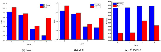
Figure 6.
The influence of hidden layer quantities on Loss, MSE, and R2 Value.
4.1.2. The Impact of Grid on Model Performance
In KAN, grid refers to a set of points distributed evenly or unevenly in the input space, used to define the segmented regions of the spline functions. The spline functions are fitted through these grid points within each segmented region. Adjusting the number and distribution of grid points can control the complexity of the spline functions. Under the settings of 6 neurons in the hidden layer, 3 layers, step size of 5, lamb = 0.01, and lamb_entropy = 2, the impact of grid point numbers ranging from 1 to 5 on the results was studied. Here, lamb is the coefficient for L1 regularization applied to the activation functions, which promotes sparsity and improves the interpretability of the network. lamb_entropy is the coefficient for the entropy regularization term, which helps to prevent overfitting and encourages smoother function approximations. Through this setup, the influence of different numbers of grid points on the model’s effectiveness can be analyzed, thereby finding the optimal grid settings to enhance the model’s accuracy and generalization.
Figure 7 shows the impact of changing the grid on the results. It can be seen that when the grid value varies between 1 and 5, the loss and MSE initially decrease and then increase, while the R2 value initially increases and then decreases. Modifying the Grid affects the training data less but has a more significant impact on the test data. When the grid number is small, increasing the grid can improve the model’s complexity, allowing it to better fit the training data. However, continuing to increase the grid number will further enhance the model’s complexity, potentially leading to overfitting. In cases of model overfitting, the model excels on the training set but underperforms on the test set, causing the loss and MSE to rise and the R2 to fall. This occurs because the model starts capturing noise and insignificant details in the training data instead of generalizing to new data.
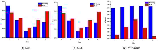
Figure 7.
The influence of grid quantity on Loss, MSE, and R2 Value.
4.1.3. The Impact of Steps on Model Performance
In KAN, steps represent the number of gradient descent updates performed during the model training process. Adjusting steps appropriately can effectively reduce training time and computational resource consumption while improving the model’s prediction accuracy and generalization ability. To study the impact of steps on the performance of the KAN model, we selected four different values: 5, 10, 15, and 20, and conducted a detailed comparative analysis of their effects. These settings help us better understand the role of Steps in optimizing model performance and identify the best parameter configuration.
Analysis of Figure 8 shows that when the steps are set to 5, 10, 15, and 20, the loss and MSE for the training set decrease as the steps increase. The most significant reduction in loss occurs when the Steps parameter increases from 5 to 15, and it slows down from 15 to 20. The R2 value increases with the number of steps, but the change is minimal, with little difference between steps 15 and 20. However, in the test set, both loss and MSE increase as the steps increase, while the R2 value decreases. This indicates that as the steps increase, the performance on the training set improves, but the performance on the test set deteriorates, leading to overfitting. This demonstrates that more steps are not always better, and it is essential to find a balance between model complexity and generalization ability.
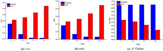
Figure 8.
The influence of step quantity on Loss, MSE, and R2 Value.
4.1.4. Impact of Hyperparameters on Computation Time
In this section, we analyze the influence of various tuning parameters, including the layer count, grid resolution, and Step magnitude, on computation time. Understanding how these hyperparameters affect the time required for training and evaluation is crucial for optimizing model performance and efficiency. We provide a detailed examination of how varying these parameters influences the overall computational cost, helping to identify configurations that balance accuracy and time efficiency.
Figure 9 shows that the running time increases linearly with the number of hidden layers, ranging from 1 to 4 layers. Specifically, when the hidden layer is 1, the running time is approximately 50 s, while increasing the hidden layers to 4 results in a running time close to 128 s. A similar trend is observed with the number of steps; when the number of steps reaches 20, the running time approaches 220 s, indicating a more pronounced upward trend. In contrast, changing the size of the grid has almost no effect on the running time, with negligible differences across various grid settings.
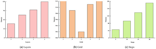
Figure 9.
Effect of hyperparameters on computation time.
Therefore, in model design, special attention should be paid to the impact of the number of hidden layers and the number of steps on running time to improve the model’s efficiency and feasibility. Optimizing these parameters can reduce computational costs while maintaining model performance. This increasing trend in computational time may pose challenges for industrial applications. Future research could explore adaptive training strategies and parallel computing to improve efficiency while maintaining accuracy.
4.2. Discussion
KAN and MLP are two different neural network models. MLP, short for Multilayer Perceptron, is a classic structure with multiple hidden layers, which achieves nonlinear mapping through connections and activation functions between neurons. In contrast, KAN is a relatively new structure that decomposes complex multivariate continuous functions into combinations of simple functions, thereby achieving efficient and theoretically sound nonlinear modeling. To better compare the performance of KAN and MLP, we varied the number of neurons and layers for each model and compared their losses and runtimes.
Figure 10 compares the performance of MLPs and KANs with 3, 4, and 5 layers. As shown in subfigure (a), KAN achieves consistently lower error and loss compared to MLP under the same number of layers and parameters. Subfigure (b) illustrates that as the number of parameters increases, the training time (in log scale) of both KAN and MLP architectures across different layers also shows an increasing trend. However, MLP exhibits a relatively moderate growth in runtime, whereas KAN experiences a more substantial increase. This difference can be attributed to their distinct computational structures: MLP relies primarily on matrix multiplications and fixed activation functions, leading to computationally efficient operations per layer. In contrast, KAN employs high-dimensional kernel mapping and spline-based activation functions, which introduce additional computational steps and resource demands as the model grows. Despite the steeper computational cost, KAN demonstrates a markedly superior decrease in loss, highlighting its advantage in modeling accuracy. This performance benefit stems from KAN’s architectural design: unlike MLPs, which use predefined activation functions (e.g., ReLU, sigmoid), KAN leverages adaptively learned spline functions over grid intervals. This allows it to better represent complex, piecewise, and non-monotonic relationships commonly found in corrosion data. For instance, variables such as water content exhibit threshold behaviors—corrosion remains minimal below a certain level but accelerates rapidly beyond it. Similarly, impurity gases like SO2 and H2S may form passivation films at low concentrations but exacerbate corrosion at higher levels. By decomposing the input space into localized spline approximations, KAN effectively captures such nonlinear and segmented patterns, providing a more expressive and mechanistically insightful model than standard MLPs.
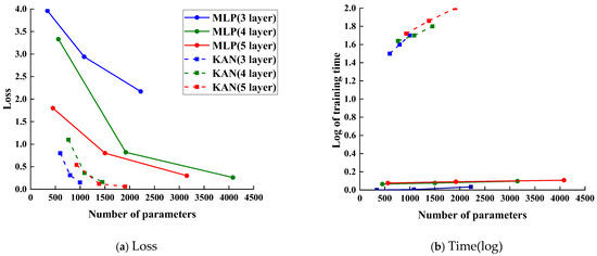
Figure 10.
Comparative Analysis of Loss and Time Between MLP and KAN Models.
To rigorously evaluate the predictive performance and generalization capability of the models, we compared KAN, MLP, RF, XGBoost, and SVR on a held-out test set that was not involved in any training or hyperparameter tuning processes. The model performance was quantified using the Coefficient of Determination (R2), which represents the proportion of variance in the dependent variable that can be explained by the independent variables, with values closer to 1 indicating better predictive accuracy.
Figure 11 compares the predictive performance of five machine learning models—KAN, MLP, RF, XGBoost, and SVR—using the Coefficient of Determination (R2) on both training and held-out test sets. As shown, the KAN model achieves the highest R2 values on both datasets, indicating its superior predictive capability and strong generalization performance. While the MLP model attains relatively high R2 on the training set, its performance on the test set is slightly lower than that of KAN, suggesting limited ability to capture complex patterns in unseen data. In contrast, RF and XGBoost demonstrate moderate R2 values, with more consistent performance between training and test sets compared to MLP. The SVR model exhibits the lowest R2 on the test set, reflecting comparatively poor predictive accuracy for the current application. Overall, these results indicate that the optimized KAN model outperforms conventional machine learning approaches in accurately modeling the target variable.
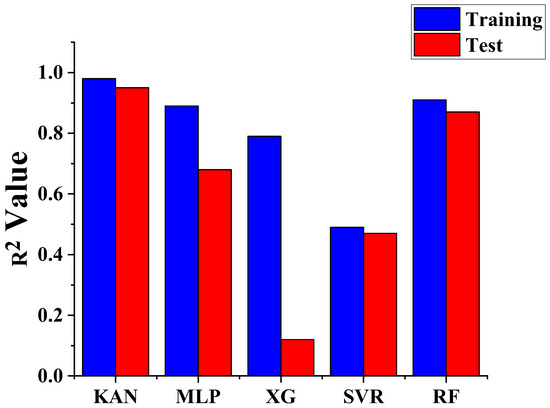
Figure 11.
R2 Performance Comparison of KAN and Conventional Machine Learning Models.
5. Conclusions
This study applied data mining and machine learning techniques to investigate the potential of Kolmogorov–Arnold Networks (KAN) for CO2 corrosion prediction. Correlation analysis identified water content, H2S, SO2, and NO2 as positively correlated with corrosion rate, while pressure showed a negative correlation. Hyperparameter sensitivity analysis revealed that a three-hidden-layer KAN with grid size 3 achieved optimal performance, and increasing the number of steps beyond a certain point did not improve accuracy but extended training time. Under comparable model complexity, KAN outperformed MLP, achieving higher prediction accuracy and lower loss with only a modest increase in computational cost. These findings demonstrate the ability of KAN to capture complex, non-linear relationships in CO2 corrosion, highlighting its potential as a robust tool for predictive corrosion modeling.
Future work should focus on further optimizing the hyperparameters of the KAN model and validating its predictive performance across diverse corrosion and operational environments. As the current model has been primarily trained on laboratory-scale or simulated datasets, extending validation to field measurements from real-world systems—such as offshore or onshore pipelines under extreme conditions—is essential to assess generalizability. Finally, practical considerations regarding computational efficiency and seamless integration into integrity management workflows will be crucial for facilitating industrial adoption.
Author Contributions
Z.D.: Conceptualization. L.Z.: Conceptualization. Y.X.: Data curation. C.G.: Data curation. W.W.: Visualization. J.Q.: Writing—original draft. M.Z.: Writing—original draft. F.W.: Supervision. G.D.: Supervision. W.L.: Supervision. All authors have read and agreed to the published version of the manuscript.
Funding
This research, which includes investigating the mechanism of rod-tubing corrosion and wear in CO2 solution based on machine learning (Project number YJSYZX23SKF0002), was funded by the Open Foundation of Shaanxi Key Laboratory of Carbon Dioxide Sequestration and Enhanced Oil Recovery. This work was also Sponsored by CNPC Innovation Fund (Grant number 2022DQ02-0201). Additionally, this research includes a project on the study of CO2 gas channeling types and regulatory policy boundaries, funded by the Research Institute of Petroleum Exploration and Development (Contract number RIPED-2024-5s-521). This work was also supported by the project (Grant number 2025ZD1406204) and the project (Grant number 2025ZD1404405).
Data Availability Statement
The original contributions presented in this study are included in the article. Further inquiries can be directed to the corresponding author.
Conflicts of Interest
Author Min Zhang was employed by the company Shangxi Yanchang Petroleum(Group) Co., Ltd, author Guoqing Dong was employed by the company Western Project Department, PetroChina Jidong Oilfield Company, Yulin, Shanxi, China, 719000. The remaining authors declare that the research was conducted in the absence of any commercial or financial relationships that could be construed as a potential conflict of interest.
Abbreviations
The following abbreviations are used in this manuscript:
| KAN | Kolmogorov–Arnold Network |
| MLP | Multilayer Perceptron |
| RF | Random Forest |
| XGBoost | Extreme Gradient Boosting |
| GBDT | Gradient Boosting Decision Tree |
| SVR | Support Vector Machine |
| R2 | Coefficient of Determination |
| MSE | Mean Squared Error |
| MAE | Mean Absolute error |
| RMSE | Root Mean Squared Error |
| PSO | Particle Swarm Optimization |
| GA | Genetic Algorithm |
| LS | Least Squares |
| CV | Cross-Validation |
References
- Zhao, Z.; Xu, K.; Xu, P.; Wang, B. CO2 corrosion behavior of simulated heat-affected zones for X80 pipeline steel. Mater. Charact. 2021, 171, 110772. [Google Scholar] [CrossRef]
- Dou, X.; He, Z.; Zhang, X.; Liu, Y.; Liu, R.; Tan, Z.; Zhang, D.; Li, Y. Corrosion behavior and mechanism of X80 pipeline steel welded joints under high shear flow fields. Colloids Surf. A Physicochem. Eng. Asp. 2023, 665, 131225. [Google Scholar] [CrossRef]
- Yevtushenko, O.; Bettge, D.; Bohraus, S.; Bäßler, R.; Pfennig, A.; Kranzmann, A. Corrosion behavior of steels for CO2 injection. Process Saf. Environ. Prot. 2014, 92, 108–118. [Google Scholar] [CrossRef]
- Pessu, F.; Barker, R.; Neville, A. Pitting and uniform corrosion of X65 carbon steel in sour environment: The influence of CO2, H2S, and temperature. Corrosion 2017, 73, 1168–1183. [Google Scholar] [CrossRef]
- Span, R.; Wagner, W. A new equation of state for carbon dioxide covering the fluid region from the triple-point temperature to 1100 K at pressures up to 800 MPa. J. Phys. Chem. Ref. Data 1996, 25, 1509–1596. [Google Scholar] [CrossRef]
- Xiang, Y.; Wang, Z.; Xu, M.; Li, Z.; Ni, W. A mechanistic model for pipeline steel corrosion in supercritical CO2-SO2-O2-H2O environments. J. Supercrit. Fluids 2013, 82, 1–12. [Google Scholar] [CrossRef]
- Choi, Y.S.; Nesic, S.; Young, D. Effect of impurities on the corrosion behavior of CO2 transmission pipeline steel in supercritical CO2-water environments. Environ. Sci. Technol. 2010, 44, 9233–9238. [Google Scholar] [CrossRef] [PubMed]
- Hua, Y.; Barker, R.; Neville, A. Understanding the influence of SO2 and O2 on the corrosion of carbon steel in water-saturated supercritical CO2. Corrosion 2015, 71, 667–683. [Google Scholar] [CrossRef]
- Newman, R. Pitting corrosion of metals. Electrochem. Soc. Interface 2010, 19, 33–38. [Google Scholar] [CrossRef]
- Sim, S.; Cole, I.; Choi, Y.-S.; Birbilis, N. A review of the protection strategies against internal corrosion for the safe transport of supercritical CO2 via steel pipeline for CCS purposes. Int. J. Greenhouse Gas Control 2014, 29, 185–199. [Google Scholar] [CrossRef]
- Gao, K.; Yu, F.; Pang, X.; Zhang, G.; Qiao, L.; Chu, W.; Lu, M. Mechanical properties of CO2 corrosion products scales and their relationship to corrosion rates. Corros. Sci. 2008, 50, 2796–2803. [Google Scholar] [CrossRef]
- Obeyesekere, N.U. Pitting corrosion. In Trends in Oil and Gas Corrosion Research and Technologies; El-Sherik, A.M., Ed.; Woodhead Publishing: Boston, MA, USA, 2017; pp. 215–248. [Google Scholar] [CrossRef]
- Doğan, B.; Altınten, A. Mathematical modeling of CO2 corrosion with NORSOK M 506. Bitlis Eren Univ. J. Sci. Technol. 2023, 12, 84–92. [Google Scholar] [CrossRef]
- Jepson, W.P.; Stitzel, S.; Kang, C.; Gopal, M. Model for sweet corrosion in horizontal multiphase slug flow. In Proceedings of the Corrosion 1997, New Orleans, LA, USA, 9–14 March 1997; OnePetro: Richardson, TX, USA, 1997. [Google Scholar] [CrossRef]
- De Waard, C.; Milliams, D.E. Carbon acid corrosion of steel. Corrosion 1975, 31, 177–181. [Google Scholar] [CrossRef]
- De Waard, C.; Lotz, U. Prediction of CO2 corrosion for carbon steel. In Proceedings of the Corrosion 1993, New Orleans, LA, USA, 7–12 March 1993; NACE: Houston, TX, USA, 1993; Volume 93, p. 69. [Google Scholar] [CrossRef]
- Wu, L.; Liao, K.; He, G.; Qin, M.; Tian, Z.; Ye, N.; Wang, M.; Leng, J. Wet gas pipeline internal general corrosion prediction based on improved De Waard 95 model. J. Pipeline Syst. Eng. Pract. 2023, 14, 04023041. [Google Scholar] [CrossRef]
- Pérez-Miguel, C.; Mendiburu, A.; Miguel-Alonso, J. Modeling the availability of Cassandra. J. Parallel Distrib. Comput. 2015, 86, 29–44. [Google Scholar] [CrossRef]
- Ricciardi, V.; Travagliati, A.; Schreiber, V.; Klomp, M.; Ivanov, V.; Augsburg, K.; Faria, C. A novel semi-empirical dynamic brake model for automotive applications. Tribol. Int. 2020, 146, 106223. [Google Scholar] [CrossRef]
- Ghorbani, Z.; Webster, R.; Lázaro, M.; Trouvé, A. Limitations in the predictive capability of pyrolysis models based on a calibrated semi-empirical approach. Fire Saf. J. 2013, 61, 274–288. [Google Scholar] [CrossRef]
- Nesic, S.; Postlethwaite, J.; Olsen, S. An electrochemical model for prediction of corrosion of mild steel in aqueous carbon dioxide solutions. Corrosion 1996, 52, 280–294. [Google Scholar] [CrossRef]
- Fellet, M.; Nyborg, R. Understanding corrosion of flexible pipes at subsea oil and gas wells. MRS Bull. 2018, 43, 654–655. [Google Scholar] [CrossRef]
- Wang, P.; Quan, Q. Prediction of corrosion rate in submarine multiphase flow pipeline based on PSO-SVR model. IOP Conf. Ser. Mater. Sci. Eng. 2019, 688, 044015. [Google Scholar] [CrossRef]
- Fang, J.; Cheng, X.; Gai, H.; Lin, S.; Lou, H. Development of machine learning algorithms for predicting internal corrosion of crude oil and natural gas pipelines. Comput. Chem. Eng. 2023, 177, 108358. [Google Scholar] [CrossRef]
- Song, Y.; Wang, Q.; Zhang, X.; Dong, L.; Bai, S.; Zeng, D.; Zhang, Z.; Zhang, H.; Xi, Y. Interpretable machine learning for maximum corrosion depth and influence factor analysis. Npj Mater. Degrad. 2023, 7, 9. [Google Scholar] [CrossRef]
- Peng, S.; Zhang, Z.; Liu, E.; Liu, W.; Qiao, W. A new hybrid algorithm model for prediction of internal corrosion rate of multiphase pipeline. J. Nat. Gas Sci. Eng. 2021, 85, 103716. [Google Scholar] [CrossRef]
- Ben Seghier, M.E.A.; Höche, D.; Zheludkevich, M. Prediction of the internal corrosion rate for oil and gas pipeline: Implementation of ensemble learning techniques. J. Nat. Gas Sci. Eng. 2022, 99, 104425. [Google Scholar] [CrossRef]
- Wang, G.; Wang, C.; Shi, L. CO2 corrosion rate prediction for submarine multiphase flow pipelines based on multi-layer perceptron. Atmosphere 2022, 13, 1833. [Google Scholar] [CrossRef]
- Wuest, T.; Weimer, D.; Irgens, C.; Thoben, K.-D. Machine learning in manufacturing: Advantages, challenges, and applications. Prod. Manuf. Res. 2016, 4, 23–45. [Google Scholar] [CrossRef]
- Liu, Z.; Wang, Y.; Vaidya, S.; Ruehle, F.; Halverson, J.; Soljačić, M.; Hou, T.Y.; Tegmark, M. KAN: Kolmogorov-Arnold networks. arXiv 2024, arXiv:2404.19756. [Google Scholar] [CrossRef]
- Mia, M.M.A.; Biswas, S.K.; Urmi, M.C.; Siddique, A. An algorithm for training multilayer perceptron (MLP) for image reconstruction using neural network without overfitting. Int. J. Sci. Technol. Res. 2015, 4, 271–275. [Google Scholar]
- Mai-Cao, L.; Truong-khac, H. A comparative study on different machine learning algorithms for petroleum production forecasting. Improv. Oil Gas Recovery 2022, 6. [Google Scholar] [CrossRef]
- Doan, T.; Vo, M.V. Using machine learning techniques for enhancing production forecast in North Malay Basin. Improv. Oil Gas Recovery 2021, 5, 2–5. [Google Scholar] [CrossRef]
- Brown, J.; Graver, B.; Gulbrandsen, E.; Dugstad, A.; Morland, B. Update of DNV recommended practice RP-J202 with focus on CO2 corrosion with impurities. Energy Procedia 2014, 63, 2432–2441. [Google Scholar] [CrossRef]
- Hua, Y.; Jonnalagadda, R.; Zhang, L.; Neville, A.; Barker, R. Assessment of general and localized corrosion behavior of X65 and 13Cr steels in water-saturated supercritical CO2 environments with SO2/O2. Int. J. Greenh. Gas Control 2017, 64, 126–136. [Google Scholar] [CrossRef]
- Sui, P.; Sun, J.; Hua, Y.; Liu, H.; Zhou, M.; Zhang, Y.; Liu, J.; Wang, Y. Effect of temperature and pressure on corrosion behavior of X65 carbon steel in water-saturated CO2 transport environments mixed with H2S. Int. J. Greenh. Gas Control 2018, 73, 60–69. [Google Scholar] [CrossRef]
- Yan, S.; Li, W.; Zhang, M.; Wang, Z.; Liu, Z.; Lin, K.; Yi, H. An innovative method for hydraulic fracture parameters optimization to enhance production in tight oil reservoirs. Improv. Oil Gas Recovery 2023, 8, 12–13. [Google Scholar] [CrossRef]
- De Winter, J.C.F.; Gosling, S.D.; Potter, J. Comparing the Pearson and Spearman correlation coefficients across distributions and sample sizes: A tutorial using simulations and empirical data. Psychol. Methods 2016, 21, 273–290. [Google Scholar] [CrossRef] [PubMed]


Disclaimer/Publisher’s Note: The statements, opinions and data contained in all publications are solely those of the individual author(s) and contributor(s) and not of MDPI and/or the editor(s). MDPI and/or the editor(s) disclaim responsibility for any injury to people or property resulting from any ideas, methods, instructions or products referred to in the content. |
© 2025 by the authors. Licensee MDPI, Basel, Switzerland. This article is an open access article distributed under the terms and conditions of the Creative Commons Attribution (CC BY) license (https://creativecommons.org/licenses/by/4.0/).