Article

Fire Resistance Prediction in FRP-Strengthened Structural Elements: Application of Advanced Modeling and Data Augmentation Techniques

1
Department of Architecture, Mimar Sinan Fine Arts University, 34427 Istanbul, Turkey
2
Department of Civil Engineering, Istanbul University-Cerrahpasa, 34320 Istanbul, Turkey
3
GameAbove College of Engineering and Technology, Eastern Michigan University, Ypsilanti, MI 48197, USA
4
College of IT Convergence, Gachon University, Seongnam 13120, Republic of Korea
*
Authors to whom correspondence should be addressed.
Processes 2025, 13(10), 3053; https://doi.org/10.3390/pr13103053
Submission received: 3 September 2025 / Revised: 18 September 2025 / Accepted: 23 September 2025 / Published: 24 September 2025
(This article belongs to the Special Issue Machine Learning Models for Sustainable Composite Materials)

Abstract

In order to ensure the earthquake safety of existing buildings, retrofitting applications come to the fore in terms of being fast and cost-effective. Among these applications, fiber-reinforced polymer (FRP) composites are widely preferred thanks to their advantages such as high strength, corrosion resistance, applicability without changing the cross-section and easy assembly. This study presents a data augmentation, modeling, and comparison-based approach to predict the fire resistance (FR) of FRP-strengthened reinforced concrete beams. The aim of this study was to explore the role of data augmentation in enhancing prediction accuracy and to find out which augmentation method provides the best prediction performance. The study utilizes an experimental dataset taken from the existing literature. The dataset contains inputs such as varying geometric dimensions and FRP-strengthening levels. Since the original dataset used in the study consisted of 49 rows, the data size was increased using augmentation methods to enhance accuracy in model training. In this study, Gaussian noise, Regression Mixup, SMOGN, Residual-based, Polynomial + Noise, PCA-based, Adversarial-like, Quantile-based, Feature Mixup, and Conditional Sampling data augmentation methods were applied to the original dataset. Using each of them, individual augmented datasets were generated. Each augmented dataset was firstly trained using eXtreme Gradient Boosting (XGBoost) with 10-fold cross-validation. After selecting the best-performing augmentation method (Adversarial-like) based on XGBoost results, the best-performing augmented dataset was later evaluated in HyperNetExplorer, a more advanced NAS tool that can find the best performing hyperparameter optimized ANN for the dataset. ANNs achieving R2 = 0.99, MSE = 22.6 on the holdout set were discovered in this stage. This whole process is unique for the FR prediction of structural elements in terms of the data augmentation and training pipeline introduced in this study.

1. Introduction

Natural disasters, corrosion, changing environmental conditions, etc., highlight the need for buildings to be constructed robustly. In addition, the durability of structures decreases over time, and when loads different from those designed for are applied to the structure, negative consequences may arise. In recent years, with the advancement of technology, the methods used to reinforce structural elements have also evolved. These methods offer higher performance than traditional building materials. Examples of these methods include using steel diagonal elements, reinforcement with fiber-reinforced polymer (FRP), etc.
FRP was first used as a reinforcement in 1975 in Russia to strengthen a wooden bridge using Glass Fiber-Reinforced Polymer (GFRP). In the 1980s, it became widespread in bridge repairs in Europe, and in the 1990s, it became widespread in maglev train structures in Japan. Japan published its first design guidelines in 1996, after which the structural use of FRP rapidly increased worldwide [1,2]. FRP materials are lightweight and easy to transport. Thanks to their high strength-to-weight ratio, they offer strength equivalent to steel at a lower weight. They are highly workable; different variations can be applied to a single or the same element. They are resistant to corrosion, making them suitable for structures exposed to aggressive and chemical effects [3,4].
There are various types of FRP used in reinforcement. Examples include Carbon Fiber-Reinforced Polymer (CFRP), Aramid Fiber-Reinforced Polymer (AFRP), Glass Fiber-Reinforced Polymer (GFRP), Basalt Fiber-Reinforced Polymer (BFRP), and the new generation of fiber-reinforced polymers such as Polyethylene Terephthalate Fiber-Reinforced Polymer (PET-FRP), etc. Table 1 gives mechanical properties of fiber-reinforced polymer (FRP) materials and steel.
Table 1 shows that fiber-reinforced polymers such as CFRP and GFRP have tensile strengths over a wide range. AFRP offers high tensile strength and a medium elastic modulus, while BFRP has a more limited strength range. Steel, on the other hand, has a significantly higher elongation capacity than the others.
Fiber-reinforced polymers (FRPs) are materials formed by combining at least two different materials and exhibiting superior properties compared to base materials. Their main components are polymer matrix (e.g., epoxy), load-bearing fibers (e.g., aramid), and additives (stabilizers, etc.) [5]. FRP is widely used in the reinforcement of many structural elements (reinforced concrete elements, floor slabs, floors, columns, block walls, etc.). Its ease of application allows it to be used effectively even in large spans, demonstrating that FRP is a versatile reinforcement solution [6]. FRP is also used in the reinforcement of wooden structures, stone structures, arches, and historic domes. Despite the advantages of FRP, its high cost, low elastic modulus, and limited ductility are notable disadvantages. The geometric details of the FRP-reinforced specimens used in this study are presented in [7].
In order to take into account the diversity of experimental data and overcome the difficulties encountered, machine learning (ML), offering high prediction accuracy, has been adopted. Various studies have been conducted in this regard.
Vu and Hoang (2016) [8] proposed a hybrid machine learning model based on least the squares support vector machine (LS-SVM) and firefly algorithm to predict the ultimate drilling capacity of FRP-reinforced concrete slabs. As a result, they achieved an RMSE = 53.19, a MAPE = 10.48, and an R2 = 0.97. Abuodeh et al. (2020) [9] used Resilient Back Propagation Neural Network (RBPNN), Recursive Feature Extraction (RFE), and Neural Interpretation Diagram (NID) to investigate the behavior of reinforced concrete beams against cutting with edge-bonded and U-wrapped FRP laminates. The RBPNN model created with the selected parameters yielded the best results (R2 = 0.85 and RMSE = 8.1). Basaran et al. (2021) [10] investigated the bond strength and development length of FRP bars embedded in concrete using Gaussian Process Regression (GPR), Artificial Neural Networks (ANN), Support Vector Machines (SVMs), Regression Tree, and Multiple Linear Regression. They achieved the highest performance (r = 0.91, RMSE = 3.03, MAPE = 0.14) using GPR. Wakjira et al. (2022) [11] used ridge regression, elastic net, least absolute shrinkage and selection operator (lasso) regression, decision trees (DT), K-nearest neighbors (KNN), random forest (RF), extreme random trees (ERTs), gradient-boosted decision trees (GBDT), AdaBoost, and extreme gradient boosting (XGBoost) models to predict the shear capacity of FRP-reinforced concrete (FRP-RC) beams. The best prediction performance (MAE = 8, MAPE = 12.9%, RMSE = 12.6, R2 = 95.3%) was achieved with XGBoost, and SHAP analysis was used to identify the most important factors affecting cutting capacity. Shen et al. (2022) [12] used machine learning models such as artificial neural networks, support vector machines, decision trees, and AdaBoost to predict the drilling and cutting resistance of FRP-reinforced concrete slabs. Among these models, AdaBoost showed the highest performance (RMSE = 29.83, MAE = 23.00, R2 = 0.99). In the study, they used SHAP analysis to observe the effect of each input variable on the drilling and cutting strength of FRP-reinforced concrete slabs. Kim et al. (2022) [13] used categorical boosting (CatBoost), XGBoost, Random Forest, and Histogram Gradient Boosting models to predict FRP-concrete bond strength. Among these models, CatBoost showed the highest performance (96.1% R2, 2.31% RMSE). The results show that the proposed model can effectively predict the FRP–concrete interface bond strength. Wang et al. (2023) [14] used ANN, XGBoost, RF, gradient boosting decision tree (GBDT), (CatBoost, light gradient boosting machine (LightGBM), and adaptive boosting (AdaBoost) to predict the shear contribution of FRP (Vf). They achieved the highest performance (RMSE = 8.98, CoV = 0.58, Avg = 1.08, integral absolute error (IAE) = 0.06) with XGBoost. Additionally, they obtained important parameters on Vf using interpretable ML. Zhang et al. (2023) [15] used 1,375 FRP-concrete direct cutting test data to filter out abnormal data with an isolation forest and trained six machine learning models: ANN, SVM, decision tree, gradient boosting, random forest, and XGBoost for predicting the ultimate condition of FRP-confined concrete. They achieved the best results (RMSE = 2.528, CoV = 0.157, avg = 1.030, IAE = 0.112) with XGBoost and examined the effect of parameters with the ANN model. Khan et al. (2024) [16] predicted the flexural capacity of FRP-strengthened reinforced concrete beams using genetic expression programming (GEP) and multiple expression programming (MEP) methods. In the study, the GEP model showed the highest performance with R = 0.98 in training and validation, and they determined the most effective variables using SHAP analysis. Alizamir et al. (2024) [17] used gradient-boosted regression tree (GBRT), RF, multilayer perceptron neural network (ANNMLP), and radial basis function neural network (ANNRBF) to predict the response of FRP-reinforced concrete. The results showed that ANNMLP improved the RMSE by 9.67–83.74% compared to other methods. Ali et al. (2024) [18] investigated the structural behavior of circular columns confined with glass fiber-reinforced polymer (GFRP) and aramid fiber-reinforced polymer (AFRP) using least squares–support vector machine and long short-term memory (LSTM). Among the models used, LSTM and bidirectional LSTM demonstrated the highest prediction accuracy (R2 = 0.992 (training) R2 = 0.945 (testing), Adjusted R2 = 0.992 (training), R2 = 0.934 (testing), RMSE = 0.017, MAE = 0.013). In the rest of the article, the literature studies on predicting the fire resistance of FRP-reinforced concrete elements are included.
Bhatt et al. (2024) [19] used support vector regression (SVR), RF regressor, and deep neural network to predict the fire resistance of FRP-reinforced concrete beams. DNN provided the highest prediction accuracy, with R = 0.96 and R2 = 0.91 for previously unseen data, while RFR provided the lowest prediction accuracy, with R = 0.91 and R2 = 0.79. Kumarawadu et al. [20] used eight ensemble and four traditional ML models to predict the fire resistance of FRP-reinforced RC beams. In this study, which utilized Bayesian optimization, k-fold cross-validation, and SHAP, the XGBoost, CatBoost, LightGBM, and GRB models demonstrated an accuracy of over 92%. Habib et al. (2025) [21] used AdaBoost, DT, Extra trees, gradient boosting, logistic regression, and RF to identifying the failure potential of FRP-reinforced concrete beams exposed to fire. These models were combined with nine data preprocessing techniques to develop 54 different model combinations, and feature importance analysis was applied. In the study, the best performance (recall = 1) was achieved with the Discretized + AdaBoost model. Wang et al. (2025) [22] used LightGBM and Genetic Programming (GP) with hyperparameter optimization performed by Genetic Algorithm to evaluate the fire resistance of FRP-reinforced concrete beams. At the end of the study, LightGBM showed higher performance than GP for fire resistance prediction (R2 = 0.923 and 0.789).
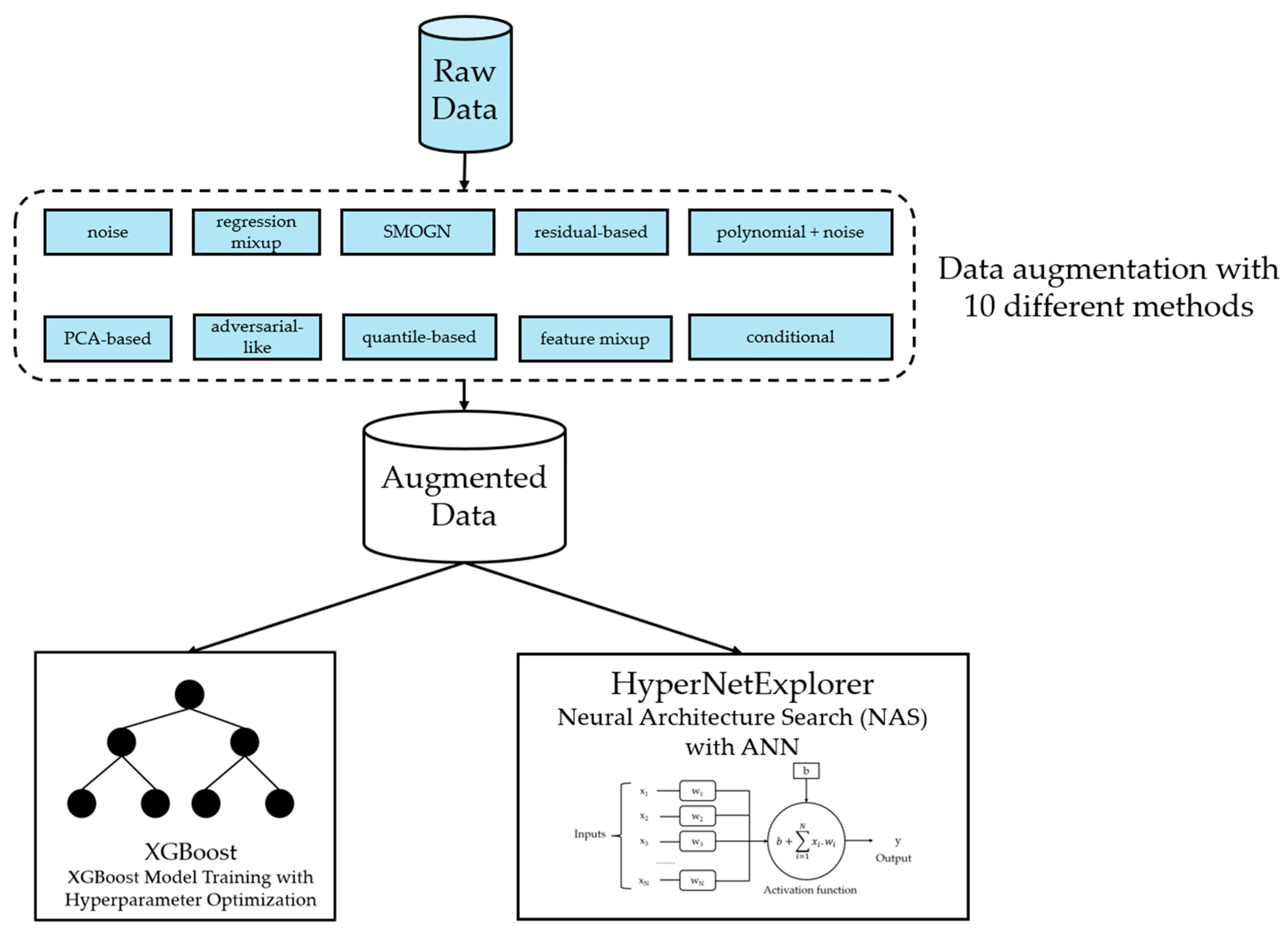
In this study, unlike other studies, 10 different data augmentation methods were applied to the dataset in [19]. Subsequently, the performance of these augmentation methods was tested using the XGBoost model with 10-fold cross-validation. Based on the results obtained, the data augmentation method with the best performance was determined, and the dataset expanded with the selected method was processed with the HyperNetExplorer tool for the model’s hyperparameter optimization. In addition, SHAP analysis was performed using XGBoost on the augmented data with the best-performing data augmentation method, and the interpretability of the model was ensured. As a result, R2 = 0.99 and MSE = 22.6 values were achieved, yielding higher results than other existing studies. This study improves the fire resistance (Fr) time prediction and increases the interpretability of ML models.

2. Materials and Methods

The study begins with the identification of the dataset on which the analysis will be performed. Once the data is obtained, data augmentation techniques are applied to increase the diversity and generalizability of the training data. The performance of the model is tested on the augmented dataset using the XGBoost algorithm with a 10-fold cross-validation method. Based on the results obtained, the data augmentation method that provided the best performance was determined. The dataset obtained using the data augmentation method that provided the best performance was tested on a web-based platform (HyperNetExplorer) to demonstrate its usability and applicability. In addition, the model’s decision mechanisms and the effects of the variables were visualized using SHAP analysis, providing a detailed explanation. Finally, the findings were compared with similar studies in the literature, and the results were discussed comprehensively.

2.1. Dataset Description

The dataset in this study was obtained from the study of Bhatt et al. [19]. The dataset consists of 49 rows. The input parameters used in the analysis of beams are as follows: beam length (L (m)), concrete cross-sectional area (Ac (mm2)), distance between the coating and steel reinforcement (Cc (mm)), steel reinforcement area in the tension zone (As (mm2)), FRP area (Af (mm2)), concrete compressive strength (fc (MPa)), steel yield strength (fy (MPa)), FRP ultimate tensile strength (fu (MPa)), FRP glass transition temperature (Tg (°C)), insulation layer thickness (tins (mm)), insulation depth on side surfaces (hi (mm)), material density (ρins (kg/m3)), thermal conductivity coefficient (kins (W/Mk)), specific heat capacity (cins (J/kg°C)), insulation thickness in anchorage regions (anc_tins) and insulation and total applied load (Ld (kN)). The output is the fire resistance time (FR (min)). All variables are numerical. Of these parameters, L, Ac, Cc, As, Af, and hi are geometric parameters, fy, fu, Tg, tins, ρins, kins, and cins are material property parameters, and Ld is the loading parameter [19,20]. Table 2 gives the first four and last rows of the dataset.
In the dataset where all variables are numerical, the data types and statistics for each variable are provided in Table 3.
The histograms shown in Figure 1 illustrate the distribution patterns of the variables in the dataset. Many variables (L, Ac, Cc, ρins, kins) exhibit a right-skewed distribution. Variables such as Ac and Af are concentrated within specific intervals.
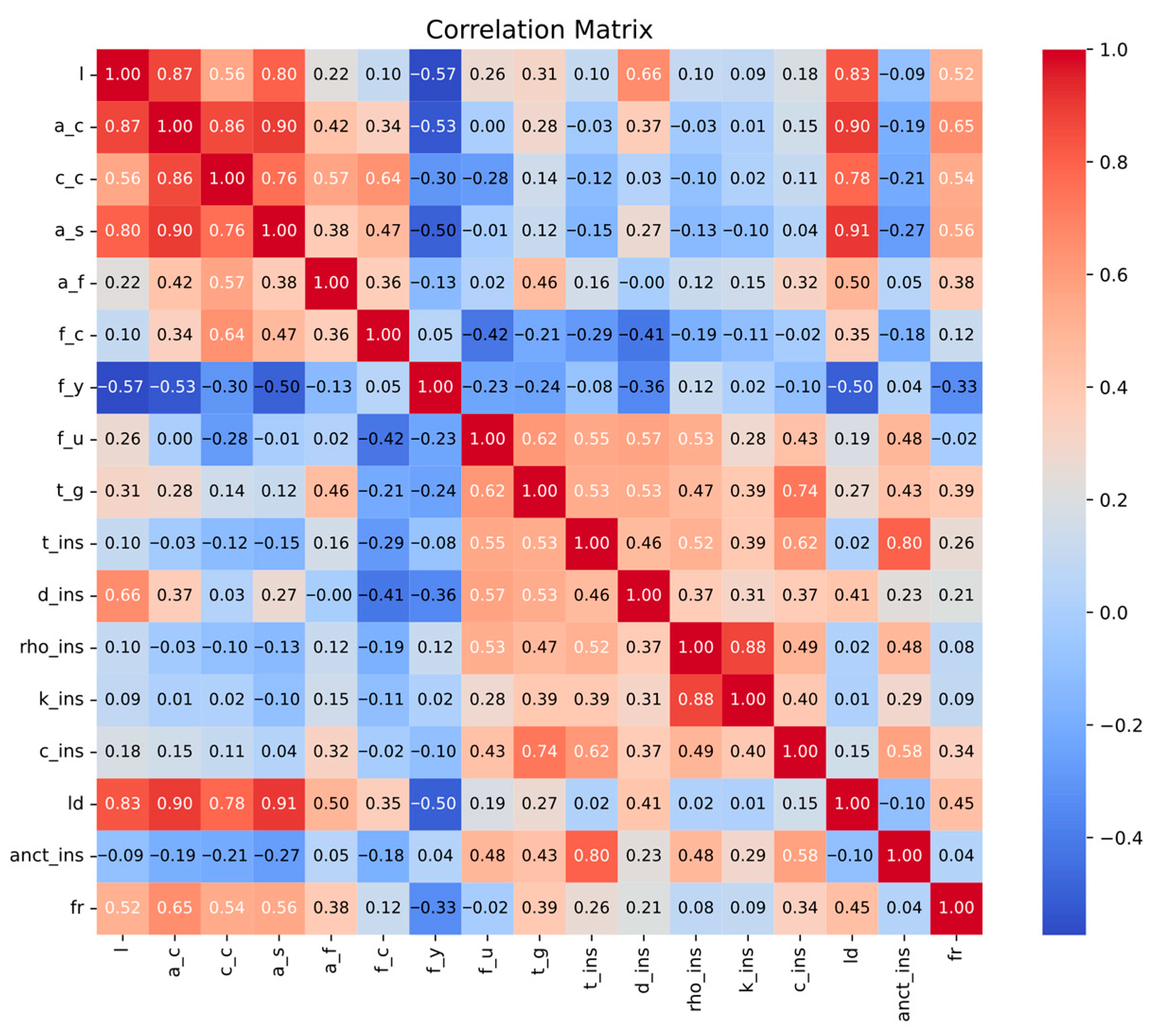
The correlation matrix in Figure 2 provides an overview of the relationships between variables in the FRP dataset. This correlation matrix helps to understand the relationships between variables in the dataset. In a correlation matrix, correlation coefficients range from −1 to +1. Strong positive or negative relationships have been observed between some variables in the matrix. For example, there is a high positive correlation of 0.91 between Ld and As. This indicates that the two variables increase together. In contrast, there is a negative correlation of −0.57 between fy and l, indicating that an increase in one variable leads to a decrease in the other. The correlation of 0.09 between the kins and L variables indicates that these two variables move independently of each other. Apart from these, most variable pairs show moderate relationships.
The dataset has 49 rows and 16 input variables. The target variable (output) is “Fr” with a mean of 109.24 and a standard deviation of 52.58. Since the data augmentation rate was set to 100%, each technique generated 1 new sample for each existing sample, adding a total of 49 new samples to the dataset. A total of 10 different augmentation techniques were applied, each working separately on the original dataset. This was performed to diversify the model’s training data and increase its generalization capacity. The model’s performance was evaluated using k-fold cross-validation, where each fold was used once as the test set while the remaining folds served as the training set.

2.2. Data Augmentation Methods Implemented

The success of machine learning models largely depends on the quality of the data and its proper preparation. Data augmentation (DA) increases data diversity by generating new samples from existing data, thereby enhancing the network’s generalization ability. This makes the dataset more resilient and provides stronger feedback to the model [23]. Data augmentation techniques applied to enrich the training set reduce the risk of overfitting and improve performance even with limited data. Adding intermediate values to continuous variables increases the model’s predictive power and helps balance underrepresented data ranges [24,25].
The raw dataset has been enriched with data augmentation methods to improve the model’s generalization ability during the training process. In this study, the data augmentation operations shown in Figure 3 have been applied. Data augmentation generates new data samples by performing transformations (e.g., mixup, noise addition, or synthetic sample generation) on the existing data. In this study, Gauss noise, Regression Mixup, SMOGN, Residual-based, Polynomial + Noise, PCA-based, Adversarial-like, Quantile-based, Feature Mixup, and Conditional Sampling methods were used to improve FRP data. Data augmentation algorithms were implemented using the Python 3.10 programming language.

2.2.1. Gaussian Noise

Gaussian noise consists of random values that follow a Gaussian probability density distribution. As the standard deviation (σ) increases, the distribution widens and the variability in the data increases. By adding this noise to nominal compositions, new samples are obtained that better represent the real components. This method doubles the size of the dataset [26]. In the study, the FRP dataset consisting of 49 rows was expanded to 98 rows using Gaussian Noise.

2.2.2. Regression Mixup

Regression Mixup is a data augmentation technique that generates synthetic data using combinations of example pairs and their labels [27]. Regression Mixup generates mixed virtual examples and soft labels, providing smoother predictions for adjacent categories but ignoring the uncertainty in mixed examples [28].

2.2.3. Synthetic Minority Over-Sampling Technique for Regression with Gaussian Noise (SMOGN)

SMOGN, a data augmentation method used in imbalanced regression problems, improves the prediction of rare values in continuous target variables and solves the problem of classification methods such as SMOTE not being suitable for regression. SMOGN is a method that expands the dataset through transformations and variations, thereby increasing the model’s learning ability and the consistency of the results [29]. SMOGN creates new data samples using random interpolation with the closest neighbors of samples belonging to the minority class [30].

2.2.4. Residual-Based

The residual-based augmentation method can be linked to the technique known in the literature as residual bootstrap. In this method, after the basic regression model is established, new samples are derived from the residual values between the model’s estimate and the actual value, and new data points reflecting the model’s errors are obtained [31,32].

2.2.5. Polynomial + Noise

In this method, polynomial terms are derived from the input variables, and small noises are added to these terms to obtain a larger dataset [33]. Data is augmented with polynomial features and noise. The method adds polynomial interactions and reduces the dimension back to its original state, capturing nonlinear relationships by adding Gaussian noise.

2.2.6. Principal Component Analysis (PCA)-Based Augmentation

Principal Component Analysis (PCA) reduces the size of the data and generates new samples from different aspects of variance [34]. The data is reduced to a low-dimensional space using PCA, noise is added to the PC coordinates, and it is reflected back to the original space using inverse transformation.

2.2.7. Adversarial-like Augmentation

In the Adversarial-like Augmentation Method, the goal is to make the model’s predictions invariant in a narrow region around the input by adding very small perturbations to the inputs. Controlled and small changes are applied to the inputs in a way that distorts the model’s predictions. This method both tests the stability of the model and increases its robustness [35]. Small perturbations are added to the inputs using the gradient of the linear model, and challenging examples are generated. By generating examples close to the decision boundary, the model is enabled to better handle uncertain situations and learn more robust feature representations.

2.2.8. Quantile-Based Sampling

Quantile-based sampling divides the target variable into quantiles and generates new samples within each quantile using interpolation. Resampling is performed by selecting samples from different quantiles in the target variable distribution; this preserves extreme values and underrepresented intervals [36].

2.2.9. Feature Mixup

A new sample is generated by mixing the features of two randomly selected samples. In mixup, labels are generated directly by the mixing ratio. It shuffles at the feature level; whether each feature is shuffled or not is determined by an independent Bernoulli trial. This, in particular, increases the interaction of independent variables [27,37].

2.2.10. Conditional Sampling

The target conditional distribution is approximated via k-nearest neighbors in space. Weighted sampling is performed within the neighborhood, and new samples are generated by adding Gaussian noise. In this method, resampling is applied when certain conditions are met (e.g., based on specific ranges of the target variable) [38,39].
Table 4 shows the data augmentation techniques and parameters used in this study.

2.3. Machine Learning

With the spread of technology and the internet today, the amount of data transferred over the network is rapidly increasing. This situation has made machine learning essential for data processing. Machine learning is a branch of artificial intelligence (AI) that enables computers to learn through experience. Algorithms extract meaningful information from raw data to make predictions about future scenarios. This involves model development, training, and testing phases; during training, algorithms learn from data, and are validated during the testing phase. Machine learning is used to increase efficiency in many areas, such as biomedical applications [40], robotic grasping control in space application [41], civil engineering [42], fault diagnosis of industrial machines [43] etc.
In this study, the Python programming language was chosen for developing machine learning applications. Python’s simple syntax, flexible structure, and rich library support are the reasons for its widespread use in creating machine learning models. Libraries such as Scikit-learn [44] and Keras [45] in particular enable the rapid and effective integration of different machine learning algorithms into projects. In addition, the Pandas [46] library provides comprehensive support for data processing and analysis processes. For all these reasons, the Python language was used to develop machine learning models in this study.

2.3.1. Extreme Gradient Boosting (XGBoost)

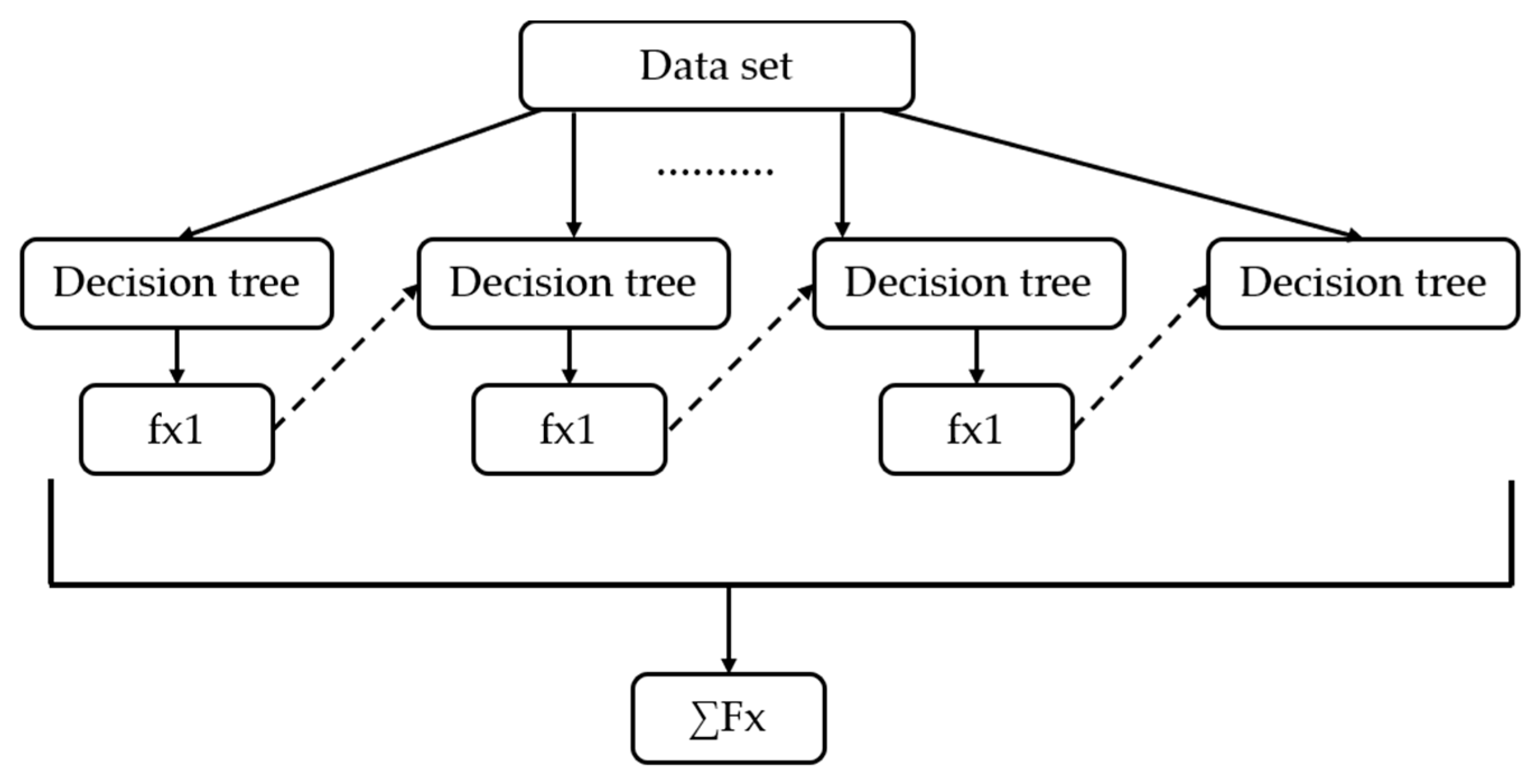
Extreme Gradient Boosting (XGBoost) is a fast and scalable implementation of the gradient boosting framework. It supports various tasks such as regression and classification, and allows users to define custom objective functions [47]. XGBoost is a widely used ensemble learning model for modeling complex relationships due to its high accuracy and efficiency [48]. The goal in XGBoost is to reduce the errors of the previous model at each step. To do this, a new decision tree is added to the model, and the updated model is used as the base learner in the next step. Through this iterative process, the outputs of weak learners are combined to create a powerful prediction model. Thanks to parallel and distributed computing support, training is both accelerated and efficient on large datasets [49,50].
The fundamental mathematical structure of XGBoost is defined by combining the outputs produced by multiple weak estimators (e.g., decision trees), and this relationship is shown in Equation (1) [51].
y l = k = 1 K f k ( x i )
In Equation (1), yl represents the predicted value for the lth observation, K represents the total number of decision trees (weak predictors), and fk (xi) represents the prediction made by the kth tree for the xi input of the ith observation. This structure demonstrates that XGBoost, as an ensemble method, produces a stronger model by combining the predictions of each tree, and that each new tree contributes to correcting the prediction errors of the previous trees (Figure 4) [51]. In the XGBoost algorithm, two of the key parameters determining the model’s performance are tree depth and number of trees [52]. Correctly determining these parameters increases the model’s learning power and shapes its generalization ability.
XGBoost has been successfully applied in studies such as predicting self-consolidating concrete properties [53] and modeling the working pressure of a cement vertical roller mill [54], among others. In this study, it was also used for fire resistance prediction in FRP-strengthened structural elements.
Hyperparameter optimization was performed to train the XGBoost model on augmented datasets with the most suitable hyperparameters and evaluate its performance using cross-validation (Table 5). K-Fold cross-validation was then applied. Thus, in each iteration, a new XGBoost model was built with the best selected hyperparameters, trained on the training data, and predictions were generated on both the training and test data. Three different performance metrics were calculated based on the prediction results. These are Root Mean Square Error (RMSE), Mean Absolute Error (MAE), and Coefficient of Determination (R2). These metrics were recorded separately for each fold. After all folds were completed, the mean and standard deviation of these metrics were taken for both training and testing.

2.3.2. K-Fold Cross Validation

K-Fold Cross-Validation was used to evaluate the model’s performance more reliably and avoid overfitting. This method ensures that the model generalizes well not only on a specific subset of the dataset but also on different subsets. The dataset is divided into K equal-sized parts, and the model is trained K times, using one part as the test set and the remaining K−1 parts as the training set in each iteration. The average of the results obtained from all iterations allows for a more accurate and balanced measurement of the model’s overall performance [55]. In this study, the K value was set to 10. In this case, the dataset was divided into ten equal parts, and the model was trained a total of ten times, using a different part as the test set each time. This ensured that each data sample was evaluated in both the training and testing phases and that the model performed consistently and generalizably across the entire dataset.

2.4. Neural Architecture Search (NAS)

Neural Architecture Search (NAS) is an AutoML domain that aims to find the optimal ANN architecture by automatically optimizing hyperparameters such as the number of layers, number of neurons, and activation functions. The search can be performed using traditional (grid/random) or adaptive optimization methods. In this study, the web-based NAS tool HyperNetExplorer (The program link will be made available upon request), developed by our research group, was used. The web-based HyperNetExplorer finds the most suitable ANN architecture for the dataset and uses various optimization algorithms from the MealPy 3.0 [56] package. The default settings are a learning rate of 0.001, 200 epochs, a population size of 20, and 50 generations; at least 1000 ANN architectures are generated in each run. The performance of the networks is monitored via the GUI, and the model with the highest accuracy is made ready for use in the production/test environment.

2.4.1. Artificial Neural Networks (ANNs)

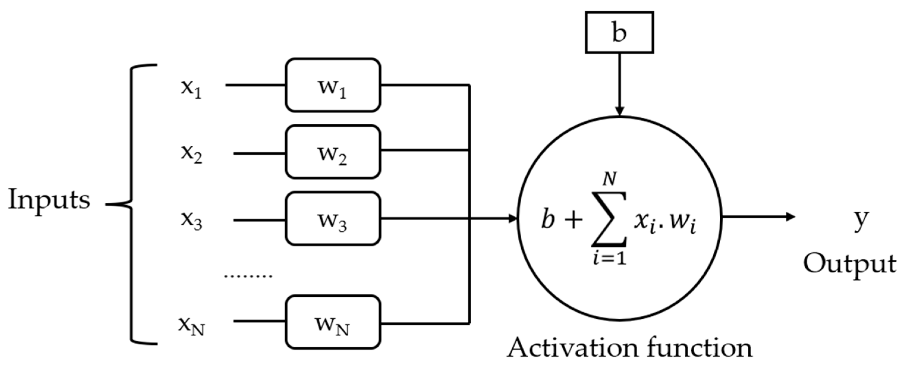
Artificial neural networks (ANNs) are computational systems that mimic the nerve cells in the human brain and learn from experience. They are based on brain research conducted in the late 1800s, and the first model was developed by McCulloch and Pitts in 1943 [57]. The basic building blocks of ANNs are artificial nerve cells. An artificial neural network consists of three layers: input, hidden, and output layers. The input layer receives data and contains neurons according to the number of parameters. The hidden layer processes the signals it receives from the input and transmits them to the output layer. The output layer then transmits the results to the outside [58]. Figure 5 shows a perceptron with N inputs xi and one output y.
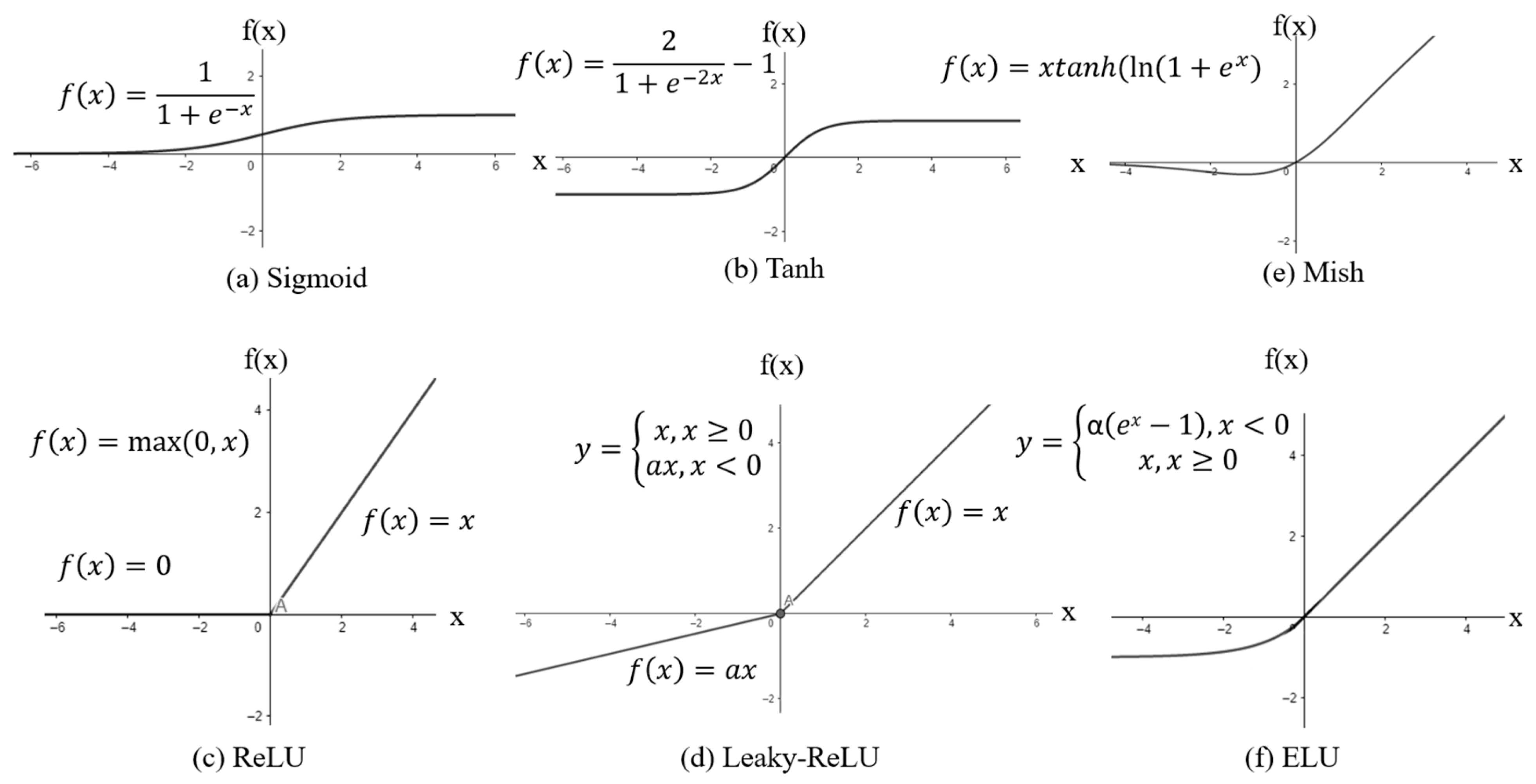
The activation function is the mechanism that processes the input to a neuron and determines its output; it is also referred to as the transfer function. Its primary role is to limit the neuron’s output to a specific range and decide whether the neuron will activate or not through a nonlinear transformation [60]. The activation functions used in this study are LeakyReLU, Sigmoid, Tanh, ReLU, LogSigmoid, ELU, and Mish (Figure 6).
Rectified Linear Unit (ReLU) is one of the most commonly used activation functions. It passes positive values as they are and sets negative values to 0 [61]. Leaky Rectified Linear Unit Function (Leaky ReLU) is a modified version of ReLU. It reduces the “dead neuron” problem by leaving a small slope at negative values [62]. Sigmoid compresses the input between 0 and 1 [63]. LogSigmoid is the logarithm of the sigmoid function. It is negative for small values and approaches 0 for large values. Tangent hyperbolic (Tanh) is similar to the sigmoid but its output ranges from −1 to 1 [64]. Exponential Linear Unit (ELU) provides soft saturation at negative values and behaves like ReLU at positive values, thereby accelerating learning [65]. Mish exhibits a slight transition at negative values and nearly linear behavior at positive values [66]. Table 6 gives HyperNetExplorer parameters to be optimized.
HyperNetExplorer utilizes metaheuristic algorithms to optimize neural network hyperparameters. In this study, the Harmony Search (HS) algorithm, a metaheuristic method inspired by jazz musicians’ improvisational performances, was employed. Developed by Geem et al. [67], HS is based on the process of finding the best harmony.

2.4.2. Harmony Search (HS)

The Harmony Search (HS) method is based on musicians trying to find the most harmonious melody through the notes they play. Tuning is the adjustment made to ensure the instrument produces the correct note. This process is carried out through iterations, similar to improvisation in music. The variables in the method are treated like notes on a musical instrument, and each solution is called a “harmony.” The algorithm uses a repetitive random search technique to replace the lowest-performing harmony in the harmony memory with a new harmony vector, thereby creating more harmonious solutions [67].
The steps of the algorithm are: determining the design parameters of the Harmony search algorithm, generating the initial Harmony matrix, developing new Harmonies, and updating the Harmony memory. The loop continues until the termination criterion is met.
In each harmony generation, the algorithm’s harmony memory consideration ratio (HMCR) is examined. HMCR is compared to a random number between 0 and 1; if it is greater, Equation (2) is used, and if it is less than or equal to, Equation (3) is used. The maximum and minimum ranges of the design variables are shown as xmin and xmax, respectively. k in Equation (3) is a randomly selected existing solution.
x i , n e w = x i , m i n + r a n d × x i , m a x x i , m i n                       i f   H M C R > r 1
x i , n e w = x i , k + r a n d × P A R x i , m a x x i , m i n               i f   H M C R r 1

2.5. Performance Metrics

Performance evaluation methods are fundamental tools used to measure the accuracy and effectiveness of machine learning models. These methods enable the quantitative assessment of a model’s success on real data. Thus, the model’s success, generalization ability, and issues such as overfitting or underfitting can be evaluated in detail. Three performance metrics (Root Mean Square Error (RMSE), Mean Absolute Error (MAE), and Coefficient of Determination (R2)) were used to evaluate the performance of the XGBoost algorithm used in this study. The aim here is to objectively and reliably measure the success of the ML model (XGBoost) applied to data augmentation data in predicting fire resistance time and to determine the most suitable model. Each metric evaluates how well the model’s prediction results match the actual values from a different perspective.

2.5.1. Root Mean Square Error (RMSE)

Root Mean Square Error (RMSE) is a metric calculated by taking the square root of the average of the squares of the model’s prediction errors. This metric gives more weight to larger errors because it squares the errors. Ideally, RMSE should be close to 0. A low RMSE value indicates that the model’s predictions are closer to the actual values. RMSE is calculated using Equation (4) [68].
R M S E = y a c t y p r e d 2 N

2.5.2. Mean Absolute Error (MAE)

Mean Absolute Error (MAE) represents the average of the absolute values of the differences between the predicted values and the actual values. Ideally, it is expected to be close to 0. A low MAE indicates that the model’s prediction errors are small. Therefore, MAE is widely used to evaluate the prediction performance of models. MAE is calculated using Equation (5) [68].
M A E = 1 N i = 1 N y a c t y p r e d

2.5.3. Coefficient of Determination (R2)

Coefficient of Determination (R2) is a statistical indicator that measures the relationship between the values predicted by the model and the actual values. It takes values between 0 and 1. R2 value close to 1 indicates that the model’s predictions closely match the actual values and that the relationship between them is strong. The mathematical expression for R2 is presented in Equation (6) [69].
R 2 = 1 i = 1 N ( y a c t y p r e d ) 2 i = 1 N ( y a c t y a v e r a g e ) 2
In the equations presented above, yact, ypred and yaverage represent the actual, predicted and average values of the observations, respectively; N denotes the number of observations.

2.6. SHapley Additive exPlanations (SHAP)

Machine learning models are powerful at extracting meaningful patterns and relationships from complex datasets, but these models are often referred to as “black-box.” This is because their internal decision-making processes can be difficult to understand and interpret. Model explainability is important for understanding the decision processes of models and why they make certain predictions. In this context, SHapley Additive exPlanations (SHAP) is a powerful and consistent method used to explain model predictions. SHAP uses Shapley values, derived from cooperative game theory, to calculate the contribution of each feature value to a single prediction [70]. Thus, the effect of each feature value on the model’s prediction can be quantitatively determined. This method quantitatively assesses the impact of each feature on the model without being sensitive to the order of the features [71].

3. Results

In this study, different data augmentation techniques were applied, and the fire resistance duration prediction performance of the XGBoost model was evaluated on the obtained datasets. The results showed significant performance differences between the techniques used. First, all techniques were compared, and the top three methods were identified. Then, the dataset generated by the data augmentation technique that yielded the best results for the XGBoost model was selected and subjected to hyperparameter optimization via HyperNetExplorer mentioned above.
The entire dataset was folded and used in both the training and testing phases. In each fold, training and testing scores were calculated separately, and then the average performance metrics (RMSE, MAE, and R2) for the entire dataset were provided. Table 7 shows the prediction performance of the XGBoost regression model on datasets created using 10 different data augmentation techniques for predicting the fire resistance time of FRP-strengthened structural elements. The performance metrics used are Root Mean Square Error (RMSE), Mean Absolute Error (MAE), and Coefficient of Determination (R2). Lower RMSE and MAE values indicate that the model’s prediction error has decreased, while a higher R2 value indicates that the model better explains the actual data.
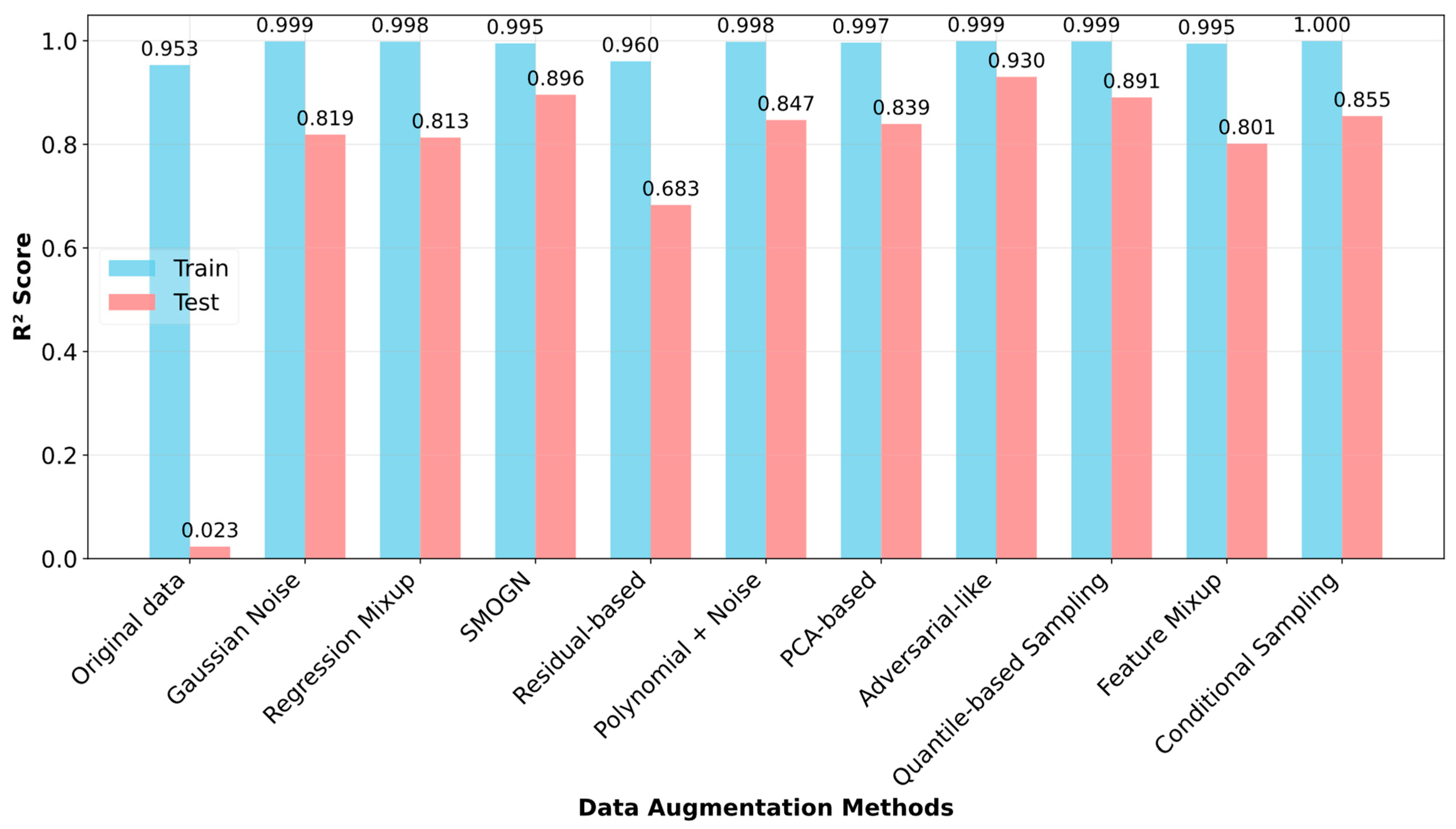
When the results in Table 7 and Figure 7 are examined, the dataset obtained using the Adversarial-like method achieved the lowest RMSE and MAE values (RMSE = 11.5936, MAE = 7.7017), demonstrating the most successful prediction performance. Additionally, the R2 value (R2 = 0.9303) obtained using this technique is higher than that of other methods. In contrast, the Residual-based method produced weaker results with relatively high error values and a low R2 value. These findings show that data augmentation methods significantly affect the fire resistance time prediction performance of the XGBoost model enhanced with FRP elements.
Among the applied methods SMOGN (Section 2.2.3), Quantile-based Augmentation (Section 2.2.8), Conditional Sampling (Section 2.2.10) takes the skewed nature of the data into account when generating the synthetic values. The performance comparison of XGBoost model’s fire resistance duration prediction of datasets generated with different augmentation methods (Table 7) indicated that the predictive performance of the datasets generated with these 3 methods were both good (i.e., high R2 values) and accurate (low variance of R2 values): SMOGN R2 = 0.8958 ± 0.1134, Quantile-based Augmentation R2 = 0.8906 ± 0.0761, Conditional Sampling R2 = 0.8546 ± 0.1070.
High variability in the R2 of the test sets was observed in three of the augmentation methods (i.e., Gaussian Noise 0.8188 ± 0.2375, Residual Based 0.6829 ± 0.1931, PCA-based 0.8394 ± 0.1961). This indicates two possible scenarios, either these augmentation methods might be introducing the synthetic samples which may not be consistently realistic or informative, or the synthetic patterns that these methods generate might not be aligning well with the XGBoost model (i.e., XGBoost might not be the best fit for these augmentations).
Following the Adversarial-like method, the quantile-based approach achieved a low error rate with RMSE = 14.78 and MAE = 10.19, and demonstrated high explanatory power in predicting fire resistance duration with an R2 = 0.8906 value. This result indicates that the technique is quite effective in improving model performance. SMIGN has slightly higher error values compared to the second technique, with RMSE = 14.91 and MAE = 11.12. However, with an R2 = 0.8958 value, it exhibits remarkable performance, particularly in terms of explanatory power. Although this technique lags slightly in terms of error values, its high R2 value contributes to reliable predictions.
The dataset augmented with the technique showing the best performance (Adversarial-like = RMSE: 11.5936, MAE:7.7017, R2: 0.9303) was analyzed in HyperNetExplor. The results are given in Table 8.
Table 8 shows that a total of 4 hidden layers (h1 = 0, 1, 2, 3) are used, with the number of neurons in each layer being 3, 512, 64, and 64, respectively. The activation functions yielding the best results are: Mish() for h1 = 0 and Tanh for h1 = 1, LogSigmoid() for h1 = 2, and LeakyReLU() for h1 = 3. This indicates that the model favors nonlinear activation functions to enable it to learn complex relationships. The performance metrics on the validation set (MSE: 50.23 and R2: 0.7) show that the model performs well on data it has not seen before. The performance metrics on the test set (MSE: 22.68, R2: 0.99) indicate that the model accurately predicts the target values in the test data.
The scatter plot in Figure 8 visualizes the machine learning test set performance of HyperNetExplorer. This figure aims to visualize the error distribution by comparing the model’s predicted values with the actual values in the holdout test set. The proximity of the green and blue points indicates the model’s success. If the points are close to each other, it means the model is making accurate predictions. The red points indicate error values. If most errors are close to 0, the model’s prediction performance is good. Although the error is higher at some points, it is generally around 0.
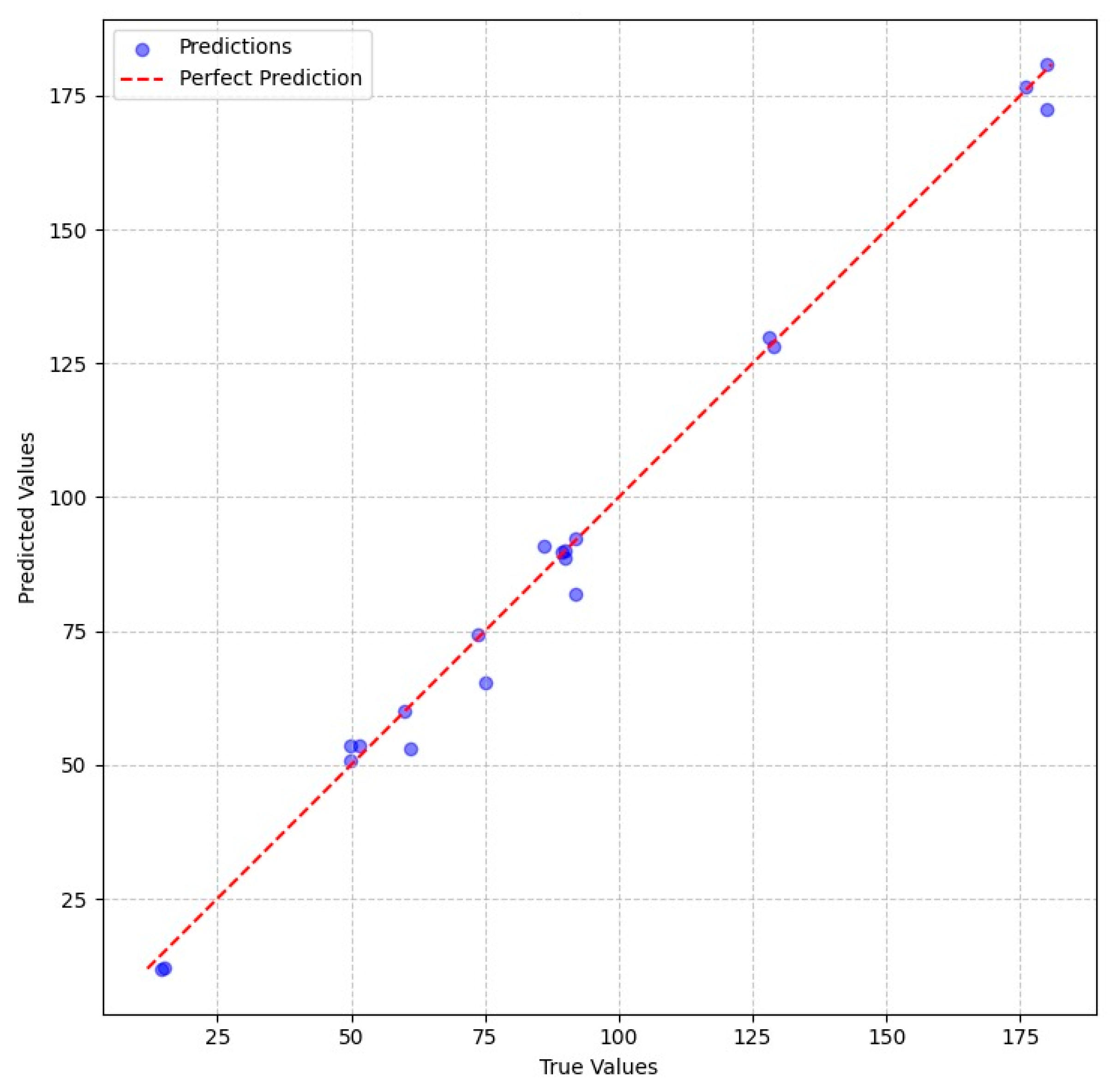
Figure 9 shows a comparison graph of Actual Values and Predicted Values used to demonstrate the model’s prediction performance. Since most of the points are very close to the red line, it can be seen that the model’s predictions are quite close to the true values. R2 = 0.99 indicates that HyperNeExplorer explains 99% of the variance and shows high fit. Mean Squared Error = 19.15 indicates that the mean squared error value is low, meaning that the prediction performance was successful.

SHapley Additive exPlanations (SHAP) Analysis

SHapley Additive exPlanations (SHAP) analysis was applied to the Adversarial-like dataset, which showed the highest performance in XGBoost analyses conducted using data augmentation techniques, to investigate the parameters affecting the fire resistance capacity of FRP-reinforced concrete beams. SHAP analysis based on XGBoost were used to understand the model’s decision mechanism. Figure 10 shows the effect of features on model predictions; the horizontal axis represents the effect, the points represent data samples, and the color gradient indicates whether the feature value is high (red) or low (blue).
Figure 10 shows that the high fy values (red dots) positively influence the model output, while low values (blue dots) negatively influence it. In other words, as fy increases, the model prediction increases. High L values (red dots) are associated with positive SHAP values and strongly contribute to predicting the fire resistance time of FRP-strengthened structural elements. High Tg values (red dots) have a positive effect, while low values have a negative effect. The inputs fy, L, and Tg have the most dominant effect on model predictions. During a fire, when the temperature exceeds the glass transition temperature (Tg) value, the mechanical properties of FRP and its adhesion to concrete rapidly decrease. This causes the FRP reinforcement to lose its effectiveness and leads to a reduction in the beam’s load-bearing capacity. Steel yield strength (fy) directly determines the load-bearing capacity of a beam exposed to fire. As beam length (L) increases, problems such as loss of rigidity become more pronounced under fire conditions.

4. Discussion

The results section shows that different data augmentation techniques significantly affect the fire resistance time prediction performance of the XGBoost model. While some techniques reduce error values, others increase the model’s explanatory power. These findings highlight the role of data augmentation methods in model accuracy and reliability. The results show that the Adversarial-like technique provides a significant performance improvement compared to other data augmentation methods. Specifically, the dataset created using the data augmentation technique that provided the best performance was subjected to hyperparameter optimization via HyperNetExplorer. This process was a critical step in improving the model’s accuracy and prediction reliability. The findings show that hyperparameter optimization, in addition to data augmentation methods, also contributes significantly to model performance.
SHAP analysis has shown that the most influential parameter in the model’s predictions is steel yield strength (fy). This finding reveals that fy plays a critical role in predicting the fire resistance duration and significantly affects model performance.
Table 9 provides a comparative summary of some important studies using ML related to FRP that are found in the literature, in terms of years, research objectives, methods used, and results obtained. This comparison aims to visually present the trends in the literature and the effectiveness of different methods, in addition to what is described in Section 1, the Introduction section. Table 9 gives the comparison of studies related to FRP in terms of year, aim, method, and results.
In this study, unlike other studies, 10 different data augmentation methods were applied to the dataset. Subsequently, the performance of these augmentation methods was tested using the XGBoost model with 10-fold cross-validation. Based on the results obtained, the data augmentation method with the best performance was identified, and the dataset expanded using the selected method was processed with the HyperNetExplorer tool for model hyperparameter optimization.
Bhatt et al. (2024) [19] used SVR, RFR, and DNN models to predict the fire resistance of FRP-reinforced concrete beams and achieved results of R = 0.96 and R2 = 0.91. Kumarawadu et al. (2024) [20] achieved over 92% accuracy using ensemble ML models such as XGBoost, CatBoost, LightGBM and GRB with a simulation-enhanced dataset. Habib et al. (2025) [21] (2025) used AdaBoost, DT, Extra Trees, Gradient Boosting, Logistic Regression, and RF to determine the damage potential of fire-exposed FRP-reinforced concrete beams. These models were combined with data preprocessing techniques to develop 54 different model combinations. In their study, the best performance was achieved with recall = 1. Wang et al. (2025) [22] used LightGBM to evaluate the fire resistance of FRP-reinforced concrete beams. At the end of their study, they achieved an R2 = 0.923 score. In contrast, in this study, based on experimental data, data augmentation and hyperparameter optimization using HyperNetExplorer resulted in an R2 = 0.99, demonstrating that even small datasets are effective for highly accurate fire resistance prediction. Furthermore, the model’s interpretability was enhanced through SHAP analysis.
The results demonstrate that the proposed model can effectively predict the fire resistance time of FRP-strengthened structural elements. Unlike previous studies, this research applied data augmentation techniques and tested them on the HyperNetExplorer. This study has achieved the highest success in FRP-fire-related studies.

5. Conclusions

In this study, the effects of different data augmentation techniques on the fire resistance duration prediction performance of the XGBoost model were systematically investigated. Ten different data augmentation methods were applied, and the model’s success was measured using the Root Mean Square Error (RMSE), Mean Absolute Error (MAE), and Coefficient of Determination (R2) metrics. The results obtained showed that data augmentation techniques significantly affected model performance. As a result of the analyses, the technique that provided the best performance was determined, and the dataset generated with this technique was subjected to hyperparameter optimization using HyperNetExplorer. As a result of the optimization, significant decreases in the model’s error values were observed, and the R2 value reached a very high level of 0.99. The MSE value was recorded as 36, indicating that the model’s prediction accuracy is quite high. These findings reveal that data augmentation techniques and hyperparameter optimization play a critical role in model accuracy and reliability. The use of HyperNetExplorer contributed to making the model suitable for real-time use.
In conclusion, the methods developed and the results obtained in this study are valuable in terms of increasing the effectiveness of the XGBoost model in predicting fire resistance time and emphasizing the importance of data augmentation and hyperparameter optimization in improving model performance in similar engineering problems. Furthermore, SHAP analysis shows that steel yield strength (fy) has the most significant effect on fire resistance time.
The main limitation of this study is the limited availability of experimental data. Although large datasets in the literature are often obtained from numerical simulations, these cannot fully reflect the variability of actual fire tests. Only one experimental dataset could be obtained in this study, and this dataset also contains a relatively small number of cases (49 experimental samples). Initial analyses showed low accuracy with this limited sample; therefore, data augmentation techniques were applied and model performance was significantly improved, and the test set R2 score increased from 0.0232 to 0.9303. Furthermore, most studies in the literature are conducted on only a single structural element [72,73], limiting the generalizability of the findings. To evaluate the generalizability of the proposed approach more comprehensively, additional studies with similar experimental setups and parameters could be conducted in the future. Future works aim to increase the diversity of the dataset by adding other parameters that affect fire resistance time in FRP-reinforced concrete elements.

Author Contributions

Conceptualization, Ü.I. and G.B.; methodology, Ü.I.; software, Ü.I.; validation, Ü.I., Y.A. and G.B.; formal analysis, Ü.I.; investigation, Ü.I. and Y.A.; resources, Ü.I.; data curation, Ü.I.; writing—original draft preparation, Y.A., Ü.I. and G.B.; writing—review and editing, C.C., Z.W.G. and G.B.; visualization, Ü.I. and C.C.; supervision, Ü.I.; project administration, G.B.; overall coordination, G.B. All authors have read and agreed to the published version of the manuscript.

Funding

This research received no external funding.

Data Availability Statement

The raw data supporting the conclusions of this article will be made available by the authors on request.

Conflicts of Interest

The authors declare no conflicts of interest.

References

  1. Taerwe, L. Non-Metallic (FRP) Reinforcement for Concrete Structures; CRC Press: Boca Raton, FL, USA, 2004. [Google Scholar] [CrossRef]
  2. Fib. Fib Model Code for Concrete Structures 2010; Wiley: Hoboken, NJ, USA, 2013. [Google Scholar] [CrossRef]
  3. Zaman, A.; Gutub, S.A.; Wafa, M.A. A review on FRP composites applications and durability concerns in the construction sector. J. Reinf. Plast. Compos. 2013, 32, 1966–1988. [Google Scholar] [CrossRef]
  4. Frigione, M.; Lettieri, M. Durability Issues and Challenges for Material Advancements in FRP Employed in the Construction Industry. Polymers 2018, 10, 247. [Google Scholar] [CrossRef]
  5. Alberto, M. Introduction of Fibre-Reinforced Polymers—Polymers and Composites: Concepts, Properties and Processes. In Fiber Reinforced Polymers—The Technology Applied for Concrete Repair; InTech: Toyama, Japan, 2013. [Google Scholar] [CrossRef]
  6. Täljsten, B. FRP strengthening of concrete structures: New inventions and applications. Prog. Struct. Eng. Mater. 2004, 6, 162–172. [Google Scholar] [CrossRef]
  7. Bhatt, P.P.; Kodur, V.K.R.; Naser, M.Z. Dataset on fire resistance analysis of FRP-strengthened concrete beams. Data Brief 2024, 52, 110031. [Google Scholar] [CrossRef]
  8. Vu, D.-T.; Hoang, N.-D. Punching shear capacity estimation of FRP-reinforced concrete slabs using a hybrid machine learning approach. Struct. Infrastruct. Eng. 2016, 12, 1153–1161. [Google Scholar] [CrossRef]
  9. Abuodeh, O.R.; Abdalla, J.A.; Hawileh, R.A. Prediction of shear strength and behavior of RC beams strengthened with externally bonded FRP sheets using machine learning techniques. Compos. Struct. 2020, 234, 111698. [Google Scholar] [CrossRef]
  10. Basaran, B.; Kalkan, I.; Bergil, E.; Erdal, E. Estimation of the FRP-concrete bond strength with code formulations and machine learning algorithms. Compos. Struct. 2021, 268, 113972. [Google Scholar] [CrossRef]
  11. Wakjira, T.G.; Al-Hamrani, A.; Ebead, U.; Alnahhal, W. Shear capacity prediction of FRP-RC beams using single and ensenble ExPlainable Machine learning models. Compos. Struct. 2022, 287, 115381. [Google Scholar] [CrossRef]
  12. Shen, Y.; Sun, J.; Liang, S. Interpretable Machine Learning Models for Punching Shear Strength Estimation of FRP Reinforced Concrete Slabs. Crystals 2022, 12, 259. [Google Scholar] [CrossRef]
  13. Kim, B.; Lee, D.-E.; Hu, G.; Natarajan, Y.; Preethaa, S.; Rathinakumar, A.P. Ensemble Machine Learning-Based Approach for Predicting of FRP—Concrete Interfacial Bonding. Mathematics 2022, 10, 231. [Google Scholar] [CrossRef]
  14. Wang, C.; Zou, X.; Sneed, L.H.; Zhang, F.; Zheng, K.; Xu, H.; Li, G. Shear strength prediction of FRP-strengthened concrete beams using interpretable machine learning. Constr. Build. Mater. 2023, 407, 133553. [Google Scholar] [CrossRef]
  15. Zhang, F.; Wang, C.; Liu, J.; Zou, X.; Sneed, L.H.; Bao, Y.; Wang, L. Prediction of FRP-concrete interfacial bond strength based on machine learning. Eng. Struct. 2023, 274, 115156. [Google Scholar] [CrossRef]
  16. Khan, M.; Khan, A.; Khan, A.U.; Shakeel, M.; Khan, K.; Alabduljabbar, H.; Najeh, T.; Gamil, Y. Intelligent prediction modeling for flexural capacity of FRP-strengthened reinforced concrete beams using machine learning algorithms. Heliyon 2024, 10, e23375. [Google Scholar] [CrossRef]
  17. Alizamir, M.; Gholampour, A.; Kim, S.; Keshtegar, B.; Jung, W. Designing a reliable machine learning system for accurately estimating the ultimate condition of FRP-confined concrete. Sci. Rep. 2024, 14, 20466. [Google Scholar] [CrossRef] [PubMed]
  18. Ali, L.; Isleem, H.F.; Bahrami, A.; Jha, I.; Zou, G.; Kumar, R.; Sadeq, A.M.; Jahami, A. Integrated behavioural analysis of FRP-confined circular columns using FEM and machine learning. Compos. Part C Open Access 2024, 13, 100444. [Google Scholar] [CrossRef]
  19. Bhatt, P.P.; Sharma, N.; Kodur, V.K.R.; Naser, M.Z. Machine learning approach for predicting fire resistance of FRP-strengthened concrete beams. Struct. Concr. 2024, 26, 4143–4165. [Google Scholar] [CrossRef]
  20. Kumarawadu, H.; Weerasinghe, P.; Perera, J.S. Evaluating the Performance of Ensemble Machine Learning Algorithms Over Traditional Machine Learning Algorithms for Predicting Fire Resistance in FRP Strengthened Concrete Beams. Electron. J. Struct. Eng. 2024, 24, 47–53. [Google Scholar] [CrossRef]
  21. Habib, A.; Barakat, S.; Al-Toubat, S.; Junaid, M.T.; Maalej, M. Developing Machine Learning Models for Identifying the Failure Potential of Fire-Exposed FRP-Strengthened Concrete Beams. Arab. J. Sci. Eng. 2025, 50, 8475–8490. [Google Scholar] [CrossRef]
  22. Wang, S.; Fu, Y.; Ban, S.; Duan, Z.; Su, J. Genetic evolutionary deep learning for fire resistance analysis in fibre-reinforced polymers strengthened reinforced concrete beams. Eng. Fail. Anal. 2025, 169, 109149. [Google Scholar] [CrossRef]
  23. Moreno-Barea, F.J.; Jerez, J.M.; Franco, L. Improving classification accuracy using data augmentation on small data sets. Expert Syst. Appl. 2020, 161, 113696. [Google Scholar] [CrossRef]
  24. Frid-Adar, M.; Klang, E.; Amitai, M.; Goldberger, J.; Greenspan, H. Synthetic data augmentation using GAN for improved liver lesion classification. In Proceedings of the 2018 IEEE 15th International Symposium on Biomedical Imaging (ISBI 2018), Washington, DC, USA, 4–7 April 2018; pp. 289–293. [Google Scholar] [CrossRef]
  25. Zhou, Y.; Guo, C.; Wang, X.; Chang, Y.; Wu, Y. A Survey on Data Augmentation in Large Model Era. arXiv 2024, arXiv:2401.15422. [Google Scholar] [CrossRef]
  26. Ye, Y.; Li, Y.; Ouyang, R.; Zhang, Z.; Tang, Y.; Bai, S. Improving machine learning based phase and hardness prediction of high-entropy alloys by using Gaussian noise augmented data. Comput. Mater. Sci. 2023, 223, 112140. [Google Scholar] [CrossRef]
  27. Zhang, H.; Cisse, M.; Dauphin, Y.N.; Lopez-Paz, D. mixup: Beyond empirical risk minimization. arXiv 2017, arXiv:1710.09412. [Google Scholar] [CrossRef]
  28. Zhang, Z.; Wang, H.; Geng, J.; Deng, X.; Jiang, W. A New Data Augmentation Method Based on Mixup and Dempster-Shafer Theory. IEEE Trans. Multimed. 2024, 26, 4998–5013. [Google Scholar] [CrossRef]
  29. Cesmeli, M.S. Increasing the prediction efficacy of the thermodynamic properties of R515B refrigerant with machine learning algorithms using SMOGN data augmentation method. Int. J. Refrig. 2025, 179, 44–59. [Google Scholar] [CrossRef]
  30. Branco, P.; Torgo, L.; Ribeiro, R.P. SMOGN: A Pre-Processing Approach for Imbalanced Regression. Available online: https://www.researchgate.net/publication/319906917 (accessed on 25 August 2025).
  31. Innocenti, S.; Matte, P.; Fortin, V.; Bernier, N. Analytical and Residual Bootstrap Methods for Parameter Uncertainty Assessment in Tidal Analysis with Temporally Correlated Noise. J. Atmos. Ocean Technol. 2022, 39, 1457–1481. [Google Scholar] [CrossRef]
  32. Friedrich, M.; Lin, Y. Sieve bootstrap inference for linear time-varying coefficient models. J. Econom. 2024, 239, 105345. [Google Scholar] [CrossRef]
  33. Huang, S.-G.; Chung, M.K.; Qiu, A. Fast mesh data augmentation via Chebyshev polynomial of spectral filtering. Neural Netw. 2021, 143, 198–208. [Google Scholar] [CrossRef] [PubMed]
  34. Sirakov, N.M.; Shahnewaz, T.; Nakhmani, A. Training Data Augmentation with Data Distilled by Principal Component Analysis. Electronics 2024, 13, 282. [Google Scholar] [CrossRef]
  35. Cho, S.; Hong, S.; Jeon, J.-J. Adaptive adversarial augmentation for molecular property prediction. Expert Syst. Appl. 2025, 270, 126512. [Google Scholar] [CrossRef]
  36. Wang, H.; Ma, Y. Optimal subsampling for quantile regression in big data. Biometrika 2021, 108, 99–112. [Google Scholar] [CrossRef]
  37. Cao, C.; Zhou, F.; Dai, Y.; Wang, J.; Zhang, K. A Survey of Mix-based Data Augmentation: Taxonomy, Methods, Applications, and Explainability. ACM Comput. Surv. 2024, 57, 1–38. [Google Scholar] [CrossRef]
  38. Majeed, A.; Hwang, S.O. CTGAN-MOS: Conditional Generative Adversarial Network Based Minority-Class-Augmented Oversampling Scheme for Imbalanced Problems. IEEE Access 2023, 11, 85878–85899. [Google Scholar] [CrossRef]
  39. Hu, T.; Tang, T.; Chen, M. Data Simulation by Resampling—A Practical Data Augmentation Algorithm for Periodical Signal Analysis-Based Fault Diagnosis. IEEE Access 2019, 7, 125133–125145. [Google Scholar] [CrossRef]
  40. Binson, V.A.; Thomas, S.; Subramoniam, M.; Arun, J.; Naveen, S.; Madhu, S. A Review of Machine Learning Algorithms for Biomedical Applications. Ann. Biomed. Eng. 2024, 52, 1159–1183. [Google Scholar] [CrossRef] [PubMed]
  41. Jahanshahi, H.; Zhu, Z.H. Review of machine learning in robotic grasping control in space application. Acta Astronaut. 2024, 220, 37–61. [Google Scholar] [CrossRef]
  42. Aydin, Y.; Bekdaş, G.; Işıkdağ, Ü.; Nigdeli, S.M. The State of Art in Machine Learning Applications in Civil Engineering. In Hybrid Metaheuristics in Structural Engineering; Springer: Berlin/Heidelberg, Germany, 2023; pp. 147–177. [Google Scholar] [CrossRef]
  43. Vashishtha, G.; Chauhan, S.; Sehri, M.; Zimroz, R.; Dumond, P.; Kumar, R.; Gupta, M.K. A roadmap to fault diagnosis of industrial machines via machine learning: A brief review. Measurement 2025, 242, 116216. [Google Scholar] [CrossRef]
  44. Pedregosa, F.; Varoquaux, G.; Gramfort, A.; Michel, V.; Thirion, B.; Grisel, O.; Blondel, M.; Müller, A.; Nothman, J.; Louppe, G.; et al. Scikit-learn: Machine learning in Python. J. Mach. Learn. Res. 2011, 12, 2825–2830. [Google Scholar] [CrossRef]
  45. Chollet, F. Keras. Available online: https://github.com/fchollet/keras (accessed on 25 January 2025).
  46. McKinney, W. Data Structures for Statistical Computing in Python. Scipy 2010, 445, 56–61. [Google Scholar] [CrossRef]
  47. Cherif, I.L.; Kortebi, A. On using eXtreme Gradient Boosting (XGBoost) Machine Learning algorithm for Home Network Traffic Classification. In Proceedings of the 2019 Wireless Days (WD), Manchester, UK, 24–26 April 2019; pp. 1–6. [Google Scholar] [CrossRef]
  48. Pande, C.B.; Egbueri, J.C.; Costache, R.; Sidek, L.M.; Wang, Q.; Alshehri, F.; Din, N.M.; Gautam, V.K.; Pal, S.C. Predictive modeling of land surface temperature (LST) based on Landsat-8 satellite data and machine learning models for sustainable development. J. Clean. Prod. 2024, 444, 141035. [Google Scholar] [CrossRef]
  49. Mitchell, R.; Adinets, A.; Rao, T.; Frank, E. Xgboost: Scalable gpu accelerated learning. arXiv 2018, arXiv:1806.11248. [Google Scholar] [CrossRef]
  50. Peng, B.; Qiu, J.; Chen, L.; Li, J.; Jiang, M.; Akkas, S.; Smirnov, E.; Israfilov, R.; Khekhnev, S.; Nikolaev, A. HarpGBDT: Optimizing Gradient Boosting Decision Tree for Parallel Efficiency. In Proceedings of the 2019 IEEE International Conference on Cluster Computing (CLUSTER), Albuquerque, NM, USA, 23–26 September 2019; pp. 1–11. [Google Scholar] [CrossRef]
  51. Chen, T.; Guestrin, C. XGBoost. In Proceedings of the 22nd ACM SIGKDD International Conference on Knowledge Discovery and Data Mining, New York, NY, USA, 13–17 August 2016; pp. 785–794. [Google Scholar] [CrossRef]
  52. Mo, H.; Sun, H.; Liu, J.; Wei, S. Developing window behavior models for residential buildings using XGBoost algorithm. Energy Build. 2019, 205, 109564. [Google Scholar] [CrossRef]
  53. el Mahdi Safhi, A.; Dabiri, H.; Soliman, A.; Khayat, K.H. Prediction of self-consolidating concrete properties using XGBoost machine learning algorithm: Rheological properties. Powder Technol. 2024, 438, 119623. [Google Scholar] [CrossRef]
  54. Fatahi, R.; Abdollahi, H.; Noaparast, M.; Hadizadeh, M. Modeling the working pressure of a cement vertical roller mill using SHAP-XGBoost: A ‘conscious lab of grinding principle’ approach. Powder Technol. 2025, 457, 120923. [Google Scholar] [CrossRef]
  55. Xun, Z.; Altalbawy, F.M.A.; Kanjariya, P.; Manjunatha, R.; Shit, D.; Nirmala, M.; Sharma, A.; Hota, S.; Shomurotova, S.; Sead, F.F.; et al. Developing a cost-effective tool for choke flow rate prediction in sub-critical oil wells using wellhead data. Sci. Rep. 2025, 15, 25825. [Google Scholar] [CrossRef]
  56. Mealpy. Available online: https://github.com/thieu1995/mealpy (accessed on 2 December 2024).
  57. McCulloch, W.S.; Pitts, W. A logical calculus of the ideas immanent in nervous activity. Bull. Math. Biophys. 1943, 5, 115–133. [Google Scholar] [CrossRef]
  58. Uzair, M.; Jamil, N. Effects of Hidden Layers on the Efficiency of Neural networks. In Proceedings of the 2020 IEEE 23rd International Multitopic Conference (INMIC), Bahawalpur, Pakistan, 5–7 November 2020; pp. 1–6. [Google Scholar] [CrossRef]
  59. Cardenas, L.L.; Mezher, A.M.; Bautista, P.A.B.; Leon, J.P.A.; Igartua, M.A. A Multimetric Predictive ANN-Based Routing Protocol for Vehicular Ad Hoc Networks. IEEE Access 2021, 9, 86037–86053. [Google Scholar] [CrossRef]
  60. Wang, Y.; Li, Y.; Song, Y.; Rong, X. The Influence of the Activation Function in a Convolution Neural Network Model of Facial Expression Recognition. Appl. Sci. 2020, 10, 1897. [Google Scholar] [CrossRef]
  61. Madhu, G.; Kautish, S.; Alnowibet, K.A.; Zawbaa, H.M.; Mohamed, A.W. NIPUNA: A Novel Optimizer Activation Function for Deep Neural Networks. Axioms 2023, 12, 246. [Google Scholar] [CrossRef]
  62. Banerjee, C.; Mukherjee, T.; Pasiliao, E. Feature representations using the reflected rectified linear unit (RReLU) activation. Big Data Min. Anal. 2020, 3, 102–120. [Google Scholar] [CrossRef]
  63. Zhang, M.; Vassiliadis, S.; Delgado-Frias, J.G. Sigmoid generators for neural computing using piecewise approximations. IEEE Trans. Comput. 1996, 45, 1045–1049. [Google Scholar] [CrossRef]
  64. Shen, S.-L.; Zhang, N.; Zhou, A.; Yin, Z.-Y. Enhancement of neural networks with an alternative activation function tanhLU. Expert. Syst. Appl. 2022, 199, 117181. [Google Scholar] [CrossRef]
  65. Kim, D.; Kim, J.; Kim, J. Elastic exponential linear units for convolutional neural networks. Neurocomputing 2020, 406, 253–266. [Google Scholar] [CrossRef]
  66. Wang, X.; Ren, H.; Wang, A. Smish: A Novel Activation Function for Deep Learning Methods. Electronics 2022, 11, 540. [Google Scholar] [CrossRef]
  67. Geem, Z.W.; Kim, J.H.; Loganathan, G.V. A New Heuristic Optimization Algorithm: Harmony Search. Simulation 2001, 76, 60–68. [Google Scholar] [CrossRef]
  68. Chai, T.; Draxler, R.R. Root mean square error (RMSE) or mean absolute error (MAE)?–Arguments against avoiding RMSE in the literature. Geosci. Model. Dev. 2014, 7, 1247–1250. [Google Scholar] [CrossRef]
  69. Zhou, W.; Yan, Z.; Zhang, L. A comparative study of 11 non-linear regression models highlighting autoencoder, DBN, and SVR, enhanced by SHAP importance analysis in soybean branching prediction. Sci. Rep. 2024, 14, 5905. [Google Scholar] [CrossRef]
  70. Lundberg, S.M.; Lee, S.I. A unified approach to interpreting model predictions. Advances in Neural Information Processing Systems. arXiv 2017, arXiv:1705.07874. [Google Scholar] [CrossRef]
  71. Ahmed, U.; Jiangbin, Z.; Almogren, A.; Sadiq, M.; Rehman, A.U.; Sadiq, M.T.; Choi, J. Hybrid bagging and boosting with SHAP based feature selection for enhanced predictive modeling in intrusion detection systems. Sci. Rep. 2024, 14, 30532. [Google Scholar] [CrossRef]
  72. Rafi, M.M.; Nadjai, A.; Ali, F. Fire resistance of carbon FRP reinforced-concrete beams. Mag. Concr. Res. 2007, 59, 245–255. [Google Scholar] [CrossRef]
  73. Ahmed, A.; Kodur, V. The experimental behavior of FRP-strengthened RC beams subjected to design fire exposure. Eng. Struct. 2011, 33, 2201–2211. [Google Scholar] [CrossRef]
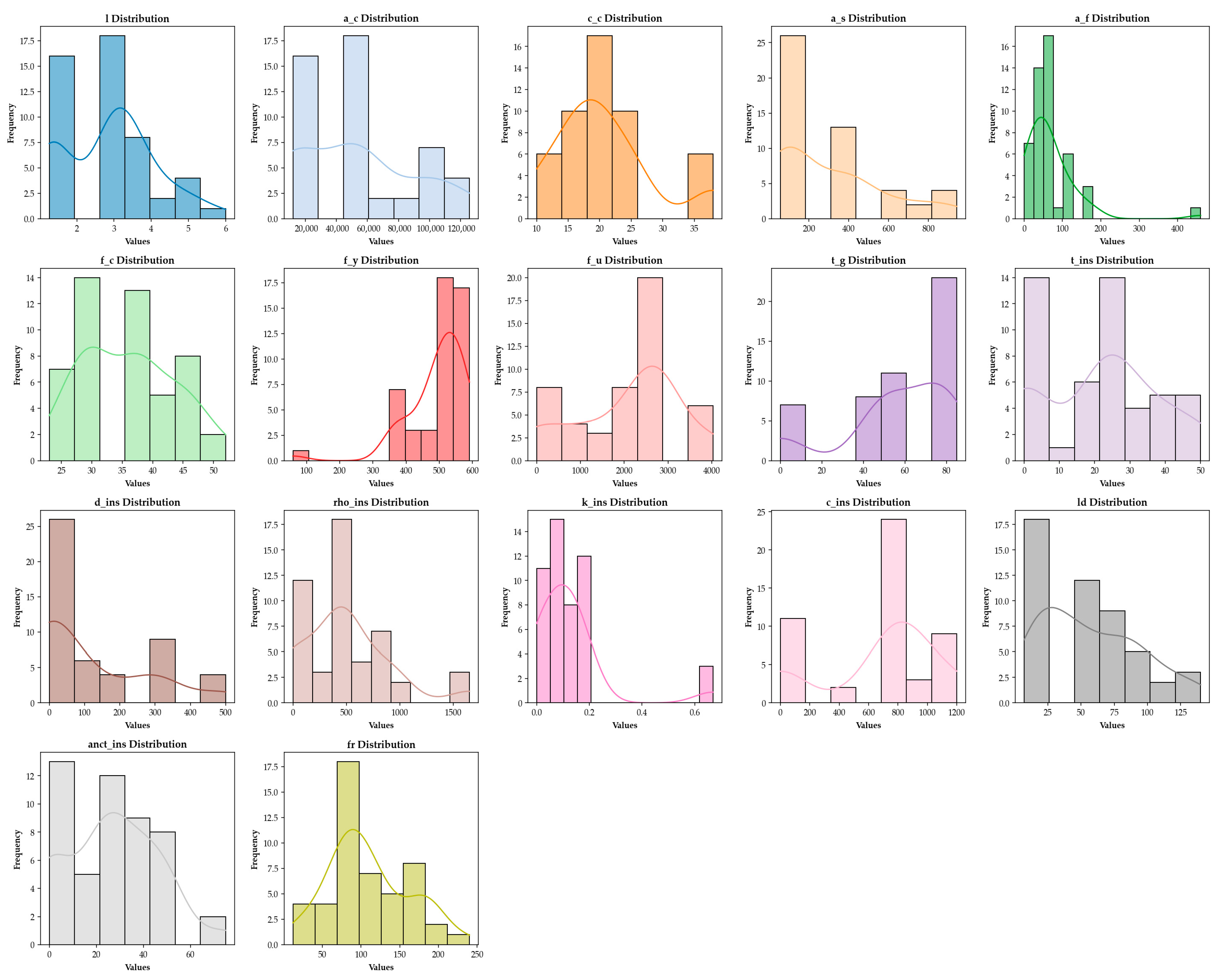
Figure 1. Histogram plots of the variables.
Processes 13 03053 g001
Figure 2. Correlation matrix.
Processes 13 03053 g002
Figure 3. Illustration of data augmentation and model training.
Processes 13 03053 g003
Figure 4. XGBoost flowchart.
Processes 13 03053 g004
Figure 5. A perceptron with N inputs xi and one output y [59].
Processes 13 03053 g005
Figure 6. Activation functions used in this study.
Processes 13 03053 g006
Figure 7. R2 scores for different data augmentation methods.
Processes 13 03053 g007
Figure 8. Scatter plot showing actual values, model predictions, and prediction errors for the holdout test set.
Processes 13 03053 g008
Figure 9. Prediction performance of the model (Actual vs. Predicted values).
Processes 13 03053 g009
Figure 10. Feature importance based on SHAP Analysis.
Processes 13 03053 g010
Table 1. Mechanical properties of fiber-reinforced polymer (FRP) materials and steel [4].
Material TypeTensile Strength (MPa)Young’s Modulus (GPa)Elongation (%)
CFRP600–392037–7840.5–1.8
GFRP483–458035–861.2–5.0
AFRP1720–362041–1751.4–4.4
BFRP600–150050–651.2–2.6
Steel483–9602006.0–12.0
Table 2. The first four and last rows of the selected dataset.
LAcCcAsAffcfyfuTgtinshiρinskinscinsLdanctinsFR
360,00025402.1047.6591000000061.2090
360,00025402.1045.5591000000061.2090
360,00025402.112044.45912800522508700.17584081.22576
360,00025402.112047.459128005240808700.17584081.24090
3.66125,73038603.210243460117282321524250.15612009732240
Table 3. Summary of data types and descriptive statistics for each variable in the selected dataset.
VariablesData TypeMinimumMaximumMeanStd. Deviation
Lfloat641.2662.84811.2468
Acint6412,000125,73053,729.959137,635.8686
Ccint64103820.73467.9445
Asfloat6456.55942.5308.1269.6602
Affloat64046067.129573.2606
fcfloat64235236.01837.6697
fyint6459591493.448993.2784
fuint64040302106.36731215.0146
Tgint6408555.979526.4610
tinsfloat6405021.765316.5583
hiint640500119.0408159.7404
ρinsint6401650497.4081422.3450
kinsfloat6400.670.12430.1532
cinsint6401200672.4285398.1558
Ldfloat647.214057.512236.9931
anctinsfloat6407526.765320.0756
FRint6412240109.244852.5886
Table 4. Data augmentation techniques and parameters.
Data Augmentation
Techniques
Parameters
Gaussian Noisenoise_factor = 0.03, augment_ratio = 1.0
Regression Mixupalpha = 0.4, augment_ratio = 1.0
SMOGNaugment_ratio = 1.0
Residual-basedaugment_ratio = 1.0
Polynomial + Noisedegree = 2, noise_factor = 0.02, augment_ratio = 1.0
PCA-basedn_components_ratio = 0.8, noise_factor = 0.05,
augment_ratio = 1.0
Adversarial-likeepsilon = 0.01, augment_ratio = 1.0
Quantile-based Samplingn_quantiles = 5, augment_ratio = 1.0
Feature Mixupmix_probability = 0.5, augment_ratio = 1.0
Conditional Samplingaugment_ratio = 1.0
Table 5. XGBoost parameters.
ParametersPossible Values
‘n_estimators’[100, 800]
‘max_depth’[3, 10]
‘learning_rate’[0.01, 0.3]
‘subsample’[0.7, 1.0]
‘colsample_bytree’[0.7, 1.0]
‘reg_alpha’[1 × 10⁻⁸, 10.0],
‘reg_lambda’[1× 10⁻⁸, 10.0]
‘min_child_weight’[1, 7]
‘random_state’[42]
‘n_jobs’[−1]
‘verbosity’[0]
Table 6. HyperNetExplorer parameters to be optimized.
ParametersRangeDescrpitons
Number of Hidden Layers (hl)0–2One hidden layer (1), Two hidden layers (2), Three hidden layers (3)
Number of Neurons in hl = 10–68 (0), 16 (1), 32 (2), 64 (3), 128 (4), 256 (5), 512 (6)
Number of Neurons in hl = 20–68 (0), 16 (1), 32 (2), 64 (3), 128 (4), 256 (5), 512 (6)
Number of Neurons in hl = 30–68 (0), 16 (1), 32 (2), 64 (3), 128 (4), 256 (5), 512 (6)
Activation Function of hl = 10–6LeakyReLU (0), Sigmoid (1), Tanh (2), ReLU (3), LogSigmoid (4), ELU (5), Mish (6)
Activation Function of hl = 20–6LeakyReLU (0), Sigmoid (1), Tanh (2), ReLU (3), LogSigmoid (4), ELU (5), Mish (6)
Activation Function of hl = 30–6LeakyReLU (0), Sigmoid (1), Tanh (2), ReLU (3), LogSigmoid (4), ELU (5), Mish (6)
Table 7. Performance comparison of XGBoost model’s fire resistance duration prediction on datasets obtained using different data augmentation techniques.
Augmented with…Data Size (Rows)SetRMSEMAER2
No method (Raw dataset)49Train11.2113 ± 0.68458.0856 ± 0.45250.9532 ± 0.0054
Test24.3087 ± 10.888519.1765 ± 7.98290.0232  ±  1.8417
Gaussian Noise98Train1.7137 ± 0.47200.4663 ± 0.09180.9988 ± 0.0004
Test16.2242 ± 4.025311.8361 ± 3.08080.8188  ±  0.2375
Regression Mixup98Train1.9247 ± 0.43760.7500 ± 0.13150.9984 ± 0.0006
Test17.8341 ± 6.413713.9886 ± 5.20020.8132  ±  0.1305
SMOGN98Train4.0179 ± 0.37322.4713 ± 0.17690.9951 ± 0.0009
Test14.9099 ± 6.704311.1190 ± 4.50700.8958  ±  0.1134
Residual-based98Train9.5594 ± 0.30646.8184 ± 0.31000.9604 ± 0.0030
Test23.1780 ± 6.06814018.3552 ± 4.66310.6829  ±  0.1931
Polynomial + Noise98Train1.9338 ± 0.37440.9237 ± 0.12940.9982 ± 0.0007
Test15.5514 ± 7.562411.9105 ± 4.73630.8470  ±  0.0859
PCA-based98Train3.0361 ± 0.34361.7367 ± 0.20970.9965 ± 0.0007
Test16.0546± 6.863512.7819 ± 5.34410.8394  ±  0.1961
Adversarial-like98Train1.2194 ± 0.19510.7302 ± 0.10970.9994 ± 0.0001
Test11.5936 ± 5.52367.7017 ± 3.05130.9303  ±  0.0731
Quantile-based Sampling94Train1.6940 ± 0.53190.3643 ± 0.09910.9987 ± 0.0005
Test14.7802 ± 7.071810.1891 ± 5.16700.8906 ± 0.0761
Feature Mixup98Train3.4956± 0.28552.3428 ± 0.20370.9945 ± 0.0010
Test17.7424 ± 4.950012.9522 ± 3.43850.8015  ±  0.1070
Conditional Sampling98Train1.0732 ± 0.35720.4413 ± 0.07850.9995 ± 0.0003
Test17.6708 ± 7.352213.9188 ± 6.53950.8546  ±  0.1070
Since the R2 values on the test set are critical for the evaluation, these values are highlighted in bold.
Table 8. HyperNetExplorer analysis results (best) of the Adversarial-like Augmented dataset.
ParametersValue
Number of Hidden Layers (hl)3
Number of Neurons in hl = 0 512
Number of Neurons in hl = 1 64
Number of Neurons in hl = 264
Number of Neurons in hl = 31024
Activation Function of hl = 0 Mish()
Activation Function of hl = 1 Tanh()
Activation Function of hl = 2LogSigmoid()
Activation Function of hl = 3LeakyReLU()
Train MSE19.18
Train R20.99
Val MSE50.23
Val R20.7
Test MSE22.68
Test R20.99
Table 9. Comparison of studies related to FRP in terms of year, aim, method, and results.
StudyYearAimMethodResult
Vu and Hoang [8]2016Predict the ultimate drilling capacity of FRP-reinforced concrete slabsleast squares support vector machine (LS-SVM) and firefly algorithmRMSE = 53.19
MAPE = 10.48
R2 = 0.97
Abuodeh et al. [9]2020Investigate the behavior of reinforced concrete beams against cutting with edge-bonded and U-wrapped FRP laminatesResilient Back Propagation Neural Network (RBPNN), Recursive Feature Extraction (RFE), and Neural Interpretation Diagram (NID)R2 = 0.85
RMSE = 8.1
Basaran et al. [10]2021Investigate the bond strength and development length of FRP bars embedded in concreteGaussian Process Regression (GPR), Artificial Neural Networks (ANN), Support Vector Machines (SVM), Regression Tree, and Multiple Linear Regressionr = 0.91
RMSE = 3.03
MAPE = 0.14
Wakjira et al. [11]2022Predict the shear capacity of FRP-reinforced concrete (FRP-RC)ridge regression, elastic net, least absolute shrinkage and selection operator (lasso) regres-sion, decision trees (DT), K-nearest neighbors (KNN), random forest (RF), extreme random trees (ERT), gradient-boosted decision trees (GBDT), AdaBoost, and extreme gradient boosting (XGBoost)MAE = 8
MAPE = 12.9%
RMSE = 12.6,
R2 = 95.3%
Kim et al. [13]2022Predict FRP-concrete bond strengthcategorical boosting (CatBoost), XGBoost, RF and Histogram Gradient BoostingR2 = 96.1% RMSE = 2.31%
Wang et al. [14]2023Predict the shear contribution of FRP (Vf).ANN, XGBoost, RF, GBDT, CatBoost, light gradient boosting machine (LightGBM), and adaptive boosting (AdaBoost)RMSE = 8.98 CoV = 0.58
Avg = 1.08
integral absolute error (IAE) = 0.06
Zhang et al. [15]2023Predict the ultimate condition of FRP-confined concreteANN, SVM, decision tree, gradient boosting, RF and XGBoostRMSE = 2.528 CoV = 0.157
avg = 1.030
IAE = 0.112
Khan et al. [16]2024Predict the flexural capacity of FRP-strengthened reinforced concrete beamsgenetic expression programming (GEP) and multiple expression programming (MEP)R = 0.98
Alizamir et al. [17]2024Predict the response of FRP-reinforced concretegradient-boosted regression tree (GBRT), RF multilayer perceptron neural network (ANNMLP), and radial basis function neural network (ANNRBF)RMSE = 9.67%
Ali et al. [18]2024Investigate the structural behavior of circular columns confined with glass fiber-reinforced polymer (GFRP) and aramid fiber-reinforced polymer (AFRP)LS-SVM and long short-term memory (LSTM)R2 = 0.992
Adj. R2 = 0.992
RMSE = 0.017 MAE = 0.013
Bhatt et al. [19]2024Predict the fire resistance of FRP-reinforced concrete beamsupport vector regression (SVR), RF regressor, and deep neural network (DNN)R = 0.96, R2 = 0.91
Kumarawadu et al. [20]2024Predict the fire resistance of FRP-reinforced RC beamsXGBoost, CatBoost, LightGBM, and GRBaccuracy > 92%
Habib et al. [21]2025Identifying the failure potential of
of FRP-reinforced concrete beams exposed to fire
AdaBoost, DT, Extra trees, Gradient boosting, Logistic regression, and RFrecall = 1
Wang et al. [22]2025Evaluate the fire resistance of FRP-reinforced concrete beams.LightGBM and GEPR2 = 0.923
This study2025Prediciton of fire resistance time of FRP-strengthened structural beamXGBoost + HyperNetExplorerR2 = 0.99
MSE = 22.6
Disclaimer/Publisher’s Note: The statements, opinions and data contained in all publications are solely those of the individual author(s) and contributor(s) and not of MDPI and/or the editor(s). MDPI and/or the editor(s) disclaim responsibility for any injury to people or property resulting from any ideas, methods, instructions or products referred to in the content.