Abstract
The high penetration of distributed generators (DGs) causes severe voltage fluctuations and voltage limit violations in distribution networks. Traditional control methods rely on precise line parameters, which are often unavailable or inaccurate, and therefore are limited in practical applications. This paper proposes a data-driven multi-mode adaptive control method with multi-region coordination to enhance the operational performance of distribution networks. First, the network is partitioned into multiple regions, each equipped with a local controller to formulate reactive power control strategies for DGs. Second, regions exchange voltage and current measurements to establish linear input–output relationships through dynamic linearization, thereby developing a multi-mode model for different control objectives. Finally, each region employs the gradient descent method to iteratively optimize its control strategy, enabling fast responses to changing operating conditions in distribution networks. Case studies on modified IEEE 33-node and 123-node test systems demonstrate that the proposed method reduces voltage deviation, load imbalance, and power loss by 31.25%, 19.17%, and 20.68%, respectively, and maintains strong scalability for application in large-scale distribution networks.
1. Introduction
The widespread integration of distributed generator (DG) systems, such as photovoltaic (PV) and wind turbine (WT) units, into distribution networks has significantly increased the complexity and variability of their operational conditions [1,2,3]. The uncertain and fluctuating output of DGs frequently causes voltage violations, reverse power flows, and increased losses in distribution networks, posing substantial challenges to operational control [4,5]. Nevertheless, DG inverters, as power electronic devices, can rapidly regulate reactive power, providing new opportunities to enhance the efficiency and flexibility of distribution network operation [6,7].
The optimization of distribution network control using the reactive power compensation capability of DG inverters has garnered widespread attention. In [8], a reactive power control method for PV inverters was proposed, where the reactive power is adaptively adjusted to reduce active power losses and alleviate overvoltage issues. In [9], a three-stage robust voltage control framework was introduced to mitigate rapid voltage deviations due to high PV penetration. A multi-objective hierarchical coordinated Volt/Var control method was presented in [10], where the PV inverter strategy was adjusted for central control and applying droop control for local control to minimize network power losses. A coordinated voltage control scheme integrating static synchronous compensators, DG inverters, and on-load tap changers was proposed in [11] to effectively suppress voltage fluctuations. In [12], a voltage and VAR control method was proposed that accelerates the solution process of physical models by applying linearization and conic relaxation, thereby meeting the demand for fast voltage control in distribution networks. These methods have effectively improved the operating performance of distribution networks. Nevertheless, most rely on precise line parameters of distribution networks, such as resistance, reactance, and load, for physical model construction. In practice, however, such parameters are often difficult to obtain or prone to large errors, which can directly lead to ineffective voltage regulation, higher operational risks, and even control failures in distribution networks [13]. These challenges underscore the urgent need for control methods that can operate reliably without depending on accurate network parameter information.
With the continuous advancement of digitalization and communication technologies, the deployment of advanced metering systems in distribution networks is becoming increasingly widespread, providing extensive measurement data on voltage, current, and power [14,15,16]. These data contain crucial information about the operational states of distribution networks and user behavior. Fully leveraging these measurement data to develop data-driven control models for distribution networks, thereby eliminating dependence on precise line parameters, has become essential to enhancing operational efficiency and control performance [17].
Research on data-driven distribution network control has increasingly become a focal point in recent years. A data-driven method was proposed in [18] to enabling adaptive control of DG inverters without requiring precise physical models. In [19], a data-driven reactive power/voltage control strategy for distributed energy resources was introduced, employing neural network learning to efficiently approximate optimal reactive power flow solutions. In [20], deep convolutional neural networks were trained on historical data to generate optimal voltage control curves for PV inverters. These studies highlight the promise of data-driven approaches in enhancing voltage regulation and power optimization. Nevertheless, most existing methods adopt centralized architectures that rely on global data for unified decision-making. In such architectures, reliance on a single controller makes complex data processing and computation prone to delays, thus compromising real-time performance [21]. Furthermore, frequent global data transmission may impose a substantial communication burden [22]. Therefore, it is imperative to explore distributed data-driven control methods to enhance the flexibility of distribution network control.
Recognizing the limitations of centralized control architectures, researchers have begun to explore distributed data-driven control architectures to achieve more flexible and reliable control. A multi-agent autonomous voltage control method was developed in [23], featuring centralized training and distributed execution, and can address voltage control problems. In [24], a multi-agent framework based on deep reinforcement learning (DRL) was proposed to cope with computational and scalability issues associated with precise system models. A dynamic voltage control method using distributed execution multi-agent deep reinforcement learning is proposed in [25], capable of effectively improving voltage levels. In [26], a multi-agent DRL algorithm is proposed to achieve decentralized optimization control of distribution grids while ensuring 100% safety. These studies have enhanced control flexibility through regional coordination. Nevertheless, most of them still rely on the coordination of a central controller and require historical data training, which can be time-consuming. Moreover, changes in system states may necessitate retraining to maintain control performance. Therefore, fully distributed, data-driven methods capable of online control remain a significant open challenge.
As illustrated in Table 1, distribution network control methods have been widely studied. Traditional model-based methods rely on precise network parameters, which are often difficult to obtain in practice. Centralized data-driven methods bear heavy computational burdens and may fail to meet real-time control requirements. Distributed data-driven methods based on DRL are time-consuming in training and require retraining when system states change. Therefore, developing fully distributed, data-driven control methods is key to solving the optimization challenges in distribution network operation.

Table 1.
Comparison between existing studies and the proposed method.
To address these challenges, this paper proposes a data-driven multi-mode adaptive control method incorporating multi-region coordination to rapidly mitigate DG fluctuations in distribution networks. First, the distribution network is partitioned into several regions, each equipped with a local controller responsible for designing reactive power output strategies for the local DGs. Second, each region exchanges voltage and current measurements to establish a linear relationship between regional inputs and outputs through dynamic linearization, thereby developing a data-driven multi-mode model to meet control demands under different scenarios. Third, each region employs the gradient descent method to optimize its own control strategy and dispatch it to improve the operating state of the distribution network. The results demonstrate that the proposed method can rapidly generate distributed strategies to cope with DG fluctuations, thereby significantly enhancing the operational flexibility of distribution networks. The main contributions can be summarized as follows.
- (1)
- A data-driven, multi-region coordinated control framework is proposed to rapidly respond to DG fluctuations. By fully leveraging multi-source measurement data, the proposed framework effectively addresses the issue of incomplete or unavailable line parameters. Moreover, through information exchange between adjacent regions and the construction of equivalent control variables, multi-region coordinated control is achieved, thereby reducing computational and communication burdens.
- (2)
- To address the heterogeneous operational requirements of distribution networks, a regional multi-mode adaptive control model is proposed. Based on voltage and current measurement data and using dynamic linearization, data models for four control modes are established: voltage control, load balancing, economic operation, and mixed control. Regions can adaptively switch between these control modes according to actual operating conditions, thereby meeting diverse control needs under different scenarios and significantly enhancing flexible operation performance of distribution network.
The remainder of this paper is organized as follows. Section 2 presents the methodology, including the framework, modeling, and solution of the proposed control strategy. Section 3 reports case studies and analysis, covering control performance, computational efficiency, robustness, and scalability. Section 4 concludes the paper.
2. Methodology
In this section, the data-driven multi-region coordinated control framework is first introduced. Then, a method is proposed for establishing multi-mode adaptive models at the regional level according to different control requirements. Subsequently, the distributed solution approach for this model is presented, followed by a discussion of its implementation procedure.
2.1. Framework of Data-Driven Multi-Region Coordinated Control
The framework of the proposed control method for distribution networks is shown in Figure 1. It primarily consists of intra-region measurement acquisition, inter-region coordination, data-driven multi-mode modeling, and control strategy optimization, as detailed below.
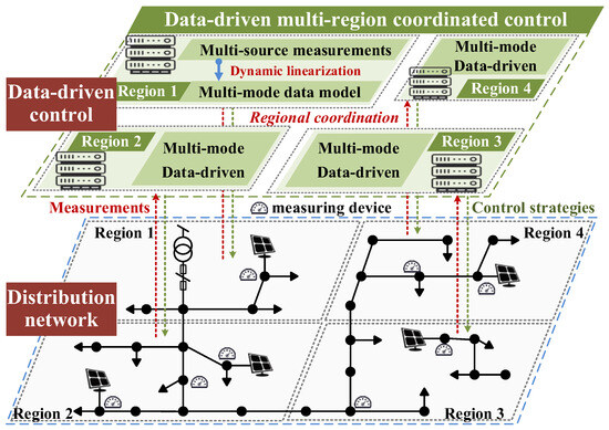
Figure 1.
Framework of data-driven multi-region coordinated control.
- (1)
- Each region of the distribution network acquires measurements of nodes and lines, including current, voltage, and power. Subsequently, regions exchange this measurement information with adjacent regions and construct a control mapping matrix using dynamic linearization to approximate the linear relationship between regional inputs and outputs.
- (2)
- Each region establishes a multi-mode adaptive control model to reduce deviation from the operating states of adjacent regions and DG output variation. The objective function is solved in parallel via gradient descent to obtain reactive power control strategies for the DGs, thereby effectively reducing computational and communication burdens.
- (3)
- Based on the actual operational requirements of different regions, four control modes are defined: voltage control, load balancing, economic operation, and mixed control. Each region adaptively selects the appropriate mode according to its operating conditions with the shared measurement data, thereby enhancing the overall operational flexibility of the distribution network.
The proposed data-driven multi-region coordinated control framework relies solely on measurement data, avoiding dependence on precise network parameters under complex operating conditions. Based on this framework, regions can switch control modes adaptively to meet dynamic power demands.
For practical operation of distribution network, edge control device is deployed in regions with compatibility for data calculation, storage, and decision-making, which can replace traditional terminal infrastructures, such as feeder terminal units. With increasing data transfer rates, the communication problems between different regions can be effectively solved. The implementation of edge control devices enables distributed operation and reduces reliance on computing resources of central controller. Meanwhile, deployed edge control devices in regions allows timely local control of the DG. With the continuous development of active distribution networks, the proposed data-driven multi-region coordinated control method will have considerable prospects for applications in practice.
2.2. Models of Multi-Mode Adaptive Control
2.2.1. Principles of Regional Partitioning
Distribution networks typically comprise a large number of nodes and exhibit complex topological structures. Partitioning these networks into distinct regions and leveraging local measurements for data-driven modeling can substantially reduce the complexity of computation.
In the context of multi-region coordinated control, each region functions as a fundamental unit for computation and control execution. An illustration of the regional partitioning and information exchange is provided in Figure 2, depicting the interactions between local controllers and their adjacent regions.
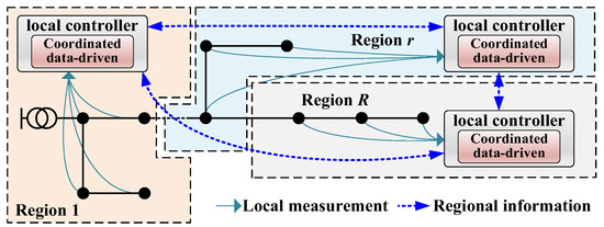
Figure 2.
Illustration of the regional partitioning and information exchange.
When partitioning the network into regions, it is essential to minimize the coupling between adjacent regions and ensure the following conditions are satisfied:
- (1)
- Regions should be delineated according to the actual topological structure or geographical location, with the number of nodes in each region kept as balanced as possible. This approach helps equalize the computation time across regions and thereby reduces the overall computational duration.
- (2)
- Each region must include at least one local controller responsible for aggregating measurement data, performing local computation, and supporting decision-making. The placement of measurement terminals must guarantee the observability of the network within each region.
- (3)
- Adjacent regions should be connected by lines without overlapping nodes. Each pair of adjacent regions shares the measurement information of the boundary lines.
Based on the above partitioning conditions, assume that the target distribution network is divided into regions. Taking region as an example, the essence of constructing the data model for region is to use operational data to describe the mapping relationship between measurement outputs and the DG strategy inputs, which can be expressed in (1):
where denotes the measurement vector of region at time , comprising current and voltage measurements. represents the unknown nonlinear mapping between the inputs and outputs of region , and denotes the vector of DG reactive power outputs in region at time . In practice, explicitly modeling this nonlinear mapping is challenging because traditional model-based approaches rely heavily on accurate network parameters, which are often unavailable or highly uncertain in practical distribution networks. Therefore, a data-driven modeling approach is adopted to approximate these complex relationships without relying on detailed network models.
2.2.2. Regional Dynamic Linearization
Dynamic linearization methods [27,28,29,30,31] are data-driven modeling techniques that rely on real-time measurements. Their core principle is to dynamically fit linear relationships between system inputs and outputs using input–output data, thereby providing a basis for data-driven control design. Measurement devices in distribution networks offer abundant multi-source data, and leveraging these data for dynamic linearization modeling effectively eliminates the dependence on precise line parameters. Based on this, regional dynamic linearization models are constructed according to measurement data of distribution network.
For the multi-region coordinated control problem of distribution networks described in Equation (1), to facilitate the linearization process, two assumptions are introduced:
Assumption 1: The partial derivative of with respect to is continuous.
Assumption 2: The input-output relationship in Equation (1) satisfies the generalized Lipschitz condition [32], implying that inputs and outputs are bounded.
These assumptions are reasonable for distribution networks, as network outputs vary continuously with inputs, and state variables such as voltage and current are constrained by operational limits, resulting in bounded responses under adjustments. This establishes a theoretical foundation for approximating the nonlinear mapping in Equation (1) with a linearized form. For detailed proofs and representative applications of these assumptions in control theory and power systems, readers are referred to [33,34].
Based on these assumptions, Equation (1) can be dynamically linearized as follows:
where denotes the estimated measurement vector of region at time , and represents the data-driven control mapping matrix for region at time , characterizing the sensitivity of the estimated measurements to the control variables. Considering the heterogeneous control objectives across multiple regions in the distribution network, different mapping matrices corresponding to various operating modes can be constructed. By evaluating deviations from the desired objectives using real-time measurement data, the control targets can be adaptively adjusted to meet the flexible operational requirements of each region.
The expression for the data-driven control mapping matrix is formulated as follows:
where is an matrix. The element denotes the entry in the -th row and -th column of . Here, represents the dimension of the measurement vector , and represents the dimension of the DG reactive power output vector .
Since this measurement-driven method relies on real-time interaction with the distribution network, minimizing the impact on system operation is essential. Therefore, an appropriate initial value for must be carefully selected. This initial value is determined based on the sensitivity between the measurement vector and the DG reactive power outputs, as expressed in the following equation:
where is the -th element of the measurement vector , and is the -th element of the DG reactive power output vector . A small change in the control variable induces a corresponding change in the measurement , from which the initial value can be computed. To minimize the impact on system, is typically set to 0.1–1% of the device’s adjustable capacity.
To achieve coordination among regions of the distribution network during the control process, the equivalent control measurements for region are defined as follows:
where represents the set of regions adjacent to region , and denotes the index of an adjacent region. can take the values of , , and , corresponding to the equivalent measurements of voltage, load, and network loss, respectively. denotes the reference measurement value for region . is the deviation coefficient for region .
2.2.3. Multi-Mode Data Model
Based on the defined regional equivalent control measurements and considering the heterogeneous control objectives and operational requirements of each region, a data-driven multi-mode adaptive model is established for each region.
- (1)
- Mode I: Voltage Control Mode
The objective of Mode I is to minimize voltage deviations and keep system voltages within an acceptable range. Its data model is given by:
where represents the equivalent voltage measurement of region at time . denotes the estimated value of the equivalent voltage measurement at time . is the voltage control mode mapping matrix for region at time . represents the change in the reactive power output of DGs in region at time .
- (2)
- Mode II: Load Balancing Mode
Different regions typically contain multiple types of loads, such as industrial, commercial, and residential loads, which may lead to load imbalances. The objective of the load balancing mode is to improve the balance among regional loads and enhance the operational efficiency of the distribution network. Its data model is formulated as:
where represents the equivalent load measurement of region at time . denotes the estimated value of this equivalent load measurement at time . is the load balancing mode mapping matrix for region at time . represents the line current measurement of region at time . denotes the maximum allowable line current for region , which typically does not exceed 500 A.
- (3)
- Mode III: Economic Operation Mode
The objective of the economic operation mode is to enhance the operational efficiency of the distribution network by reducing network losses when voltage and load are within reasonable ranges. Hence, network losses are characterized by the square of the line current, as power loss is proportional to this quantity. The corresponding data model is formulated as follows:
where represents the equivalent network loss measurement of region at time ; denotes the estimated value of this equivalent network loss measurement at time ; is economic operation mode mapping matrix for region at time .
- (4)
- Mode IV: Mixed Control Mode
In practical distribution network operations, voltage violations and load imbalances may occur simultaneously. Therefore, a mixed control mode is developed to address these combined issues, and its data model is formulated as follows:
where represents the equivalent mixed measurement of region at time ; denotes the estimated value of this equivalent mixed measurement at time ; is the mixed control mode mapping matrix for region at time .
- (5)
- Objective function in multi-mode
The objective function for region is shown in Equations (13)–(19), where represents the multimode operational objective, and denotes the penalty term for the control strategy. to denote the 2-norms of the equivalent measurements defined in Equation (5) under each control mode, aiming to minimize deviations from neighboring regions and reference values.
where is the weighting factor that penalizes variations in the input. To enable adaptive mode selection, , , , and are introduced as mode flags. It is assumed that region is operated in one mode at any period [35]. A dynamic triggering mechanism is subsequently developed for mode switching according to real-time measurements and state variations, where corresponding mode flags are shown in (20) and (21).
where represents the set of control modes. and define the voltage regulation range. is the load switching threshold.
The dynamic triggering mechanism (20) and (21) is developed for mode switching adaptively. Figure 3 shows the mode switching logic, in which mode transition process can be triggered by twelve switching conditions. Assuming that the initial operating mode is Mode III, if a voltage violation occurs, condition C1 is satisfied and Mode I will be activated and remain in effect until violation is mitigated. Taking the switching sequence Mode III–IV–I–III as an example, the operating mode initially operates in Mode III. Mode IV is selected for DG inverter while both voltage and current violations occur simultaneously. If the voltage violation still persists after DG management, the operating mode will be switched to Mode I. Once the voltage violation is eliminated, Mode III is reactivated. Therefore, adaptive mode switch can be achieved to adjust DG inverter strategy, which improves flexible operation performance of distribution network.
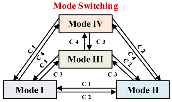
Figure 3.
Diagram of mode switching logic.
2.3. Solution for Data-Driven Control Strategy
2.3.1. Mode Mapping Matrix Update
The mode mapping matrices , , , and are crucial for solving the control strategy. In the objective function given by Equations (13)–(19), these mode mapping matrices remain unknown. Therefore, before using the objective function to derive the control strategy, these matrices must first be determined.
To address different control objectives, the corresponding mode mapping matrices are solved separately. To simplify the notation, a general symbol is introduced to represent different mode mapping matrices. Here, can take the values of , , , and , corresponding to the different operating modes.
To balance between the real-time requirements of distribution network operation control and the robustness of the mode mapping matrix, this study proposes the following estimation criterion:
where , and is the weight coefficient for the mode mapping matrix of region .
Using the gradient descent method to solve Equation (22) and by simplifying the matrix inversion step, the iterative update formula for is derived as follows:
where is the estimated value of the mode mapping matrix , and is the weight coefficient.
Furthermore, to enhance the algorithm’s ability to track the dynamic parameter , a correction equation is introduced as follows:
where is the initial value of , and are the correction thresholds for .
Thus, by utilizing voltage and current measurement data, the mode mapping matrix can be dynamically updated, thereby achieving a real-time fitting of the input–output relationship within distribution network regions.
2.3.2. Distributed Solution of Control Strategies
Based on the updated mode mapping matrix, each region applies the gradient descent method to solve the objective function given by Equations (13)–(19), deriving the iterative calculation formula for the DG reactive power output as follows:
where is the step factor for region , is the weighting factor. Note that reducing or increasing can accelerate convergence but may also increase overshoot.
Furthermore, considering the constraints on the DG reactive power output, additional corrections are applied to the control strategy derived from Equation (25):
where and represent the maximum and minimum of DG output in region , respectively.
To prevent frequent actions of DG inverters, the additional condition (28) is introduced as follows:
where is a column vector with entries equal to 1.0, and is a constant, typically assigned a value of 0.02
When condition (28) is satisfied, it indicates that under the economic operation mode (Mode III), the voltage quality is already satisfactory. In this case, there is no need to compute a new control strategy, and the mode mapping matrix and DG control strategy of region remain identical to those of the previous time step, as expressed in (29) and (30):
where and denote the economic operation mode mapping matrix and control strategy of region at time , respectively.
By incorporating condition (28) together with the update method (29) and (30), the number of DG inverter operations can be effectively reduced, thereby alleviating the computational and communication burden of regional controllers.
The establishment and solution of the multi-mode data model have been completed. A detailed theoretical analysis of the convergence and consistency of the data-driven models for each region is provided in the Appendix A.
2.3.3. Implementation of Control Strategies
The flow diagram of the proposed method is shown in Figure 4, and the detailed implementation steps are as follows:
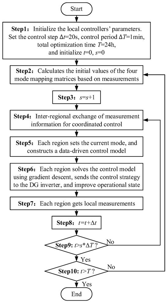
Figure 4.
Implementation of data-driven control strategies.
- (1)
- The control device in each region initializes the parameters, as shown in Step1.
- (2)
- The regional measurement devices collect voltage and current data and use them to calculate the initial values of the four mode mapping matrices, as shown in Step2.
- (3)
- Each region exchanges information with its adjacent regions to establish a data-driven model. These models are solved in a distributed manner, and the resulting reactive power control strategies for DGs are sent to their corresponding inverters, thereby improving the operational state, as shown from Step3 to Step6.
- (4)
- Each region acquires new voltage and current measurements, as shown in Step7.
- (5)
- Each region initiates a new control cycle based on the updated measurement data, as shown in Step8, returning to Step2. This iterative process continues until the system operational control t reaches the preset total time T, as shown in Step10 until End.
Note that when the network topology changes significantly, the initial values of the control mapping matrix can be recalculated to maintain control continuity.
If discrete devices such as on-load tap changers (OLTCs) are also included in distribution network, the proposed data-driven modeling can be extended across different time scales to enable hierarchical control with DG inverters.
Furthermore, as data quality is critical for data-driven methods, online identification techniques [36] can be applied to address erroneous or missing data for reliable control.
3. Case Studies and Analysis
The effectiveness of the proposed method is verified on a modified IEEE 33-node distribution test system. The method is implemented on the MATLAB R2020a platform (MathWorks, Natick, MA, USA), and the computational experiments are conducted on a computer equipped with an Intel Core i7 @ 3.20 GHz processor (Intel Corporation, Santa Clara, CA, USA) and 16 GB of RAM.
3.1. Modified IEEE 33-Node Distribution Network
The topology and partitioning of the modified IEEE 33-node distribution network are illustrated in Figure 5. The system consists of 32 lines with a rated voltage of 12.66 kV. The total active power load is 3715.0 kW, and the total reactive power load is 2300.0 kVAr. The system integrates 12 groups of PV units and 6 groups of WT units, resulting in a DG penetration level of 81%. The parameters of DG inverters are detailed in Table 2. The fluctuation profiles of DGs and loads are shown in Figure 6, with a sampling interval of 1 min.
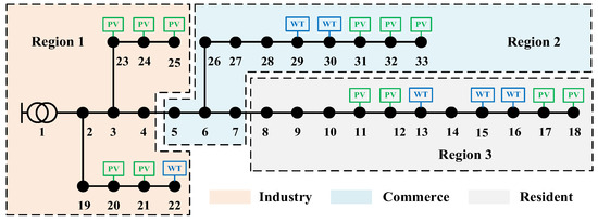
Figure 5.
Modified IEEE 33-node distribution network topology and partitioning.
Table 2.
DG inverter parameters.
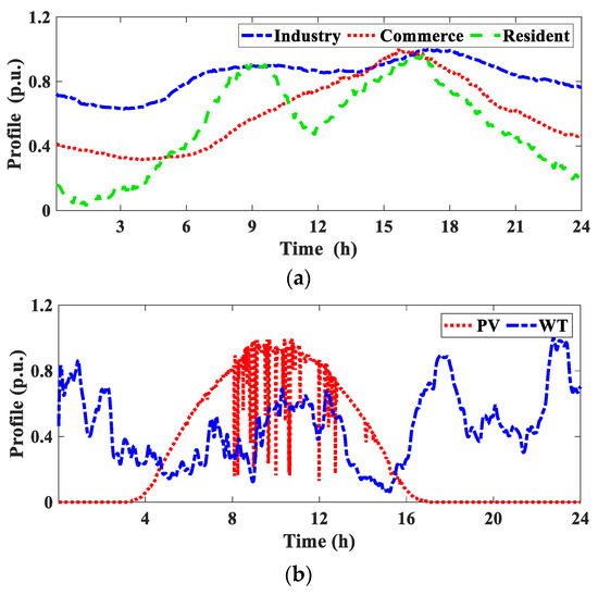
Figure 6.
Loads and DGs fluctuation curves. (a) Loads; (b) DGs.
For the three regions, the total optimization horizon is set to 24 h, with an optimization step of 1 min and a control step of 20 s. Here, represents the interval during which the source–load state is assumed to remain unchanged, whereas defines the execution interval between two consecutive control actions. For all case studies in this work, the parameters are set to , , , and . In this study, the system frequency is assumed to remain constant, as distribution networks are strongly supported by the main grid.
In order to thoroughly assess the unpredictability associated with DGs and to substantiate the effectiveness of the proposed method, a detailed analysis of four distinct scenarios is conducted:
Scenario I: The system’s initial operational state is established without DG management.
Scenario II: The proposed data-driven multi-region coordinated control method for DGs is applied.
Scenario III: The centralized data-driven control method for DGs is applied [18].
Scenario IV: The model-based optimization method for DGs is applied [12].
To provide a clearer description of the test environment and facilitate the assessment of scalability and system complexity, a comparative summary of the four scenarios is presented in Table 3. Under the same number of nodes and DG units, Scenario II employs more controllers compared with the centralized architectures in Scenarios III and IV. Consequently, each controller in Scenario II manages fewer nodes and communication links, which helps alleviate computational and communication burdens.
Table 3.
Comparative summary of the test environments in the four scenarios.
3.2. Multi-Mode Control Effect Analysis
Figure 7 illustrates the daily operating modes across the three regions. The white, gray, black, and dark gray grids represent voltage control, load balancing, economic operation, and mixed control modes, respectively. Voltage control is concentrated in Regions II and III, particularly between 14:00 and 18:00, owing to a significant increase in WT output in the afternoon, which raises node voltages beyond their upper limits and necessitates voltage regulation to mitigate overvoltage. Economic operation dominates most of the 24 h period, while load balancing and mixed control modes appear sporadically. These results demonstrate that the proposed method can adaptively identify the operational needs of each region and select the corresponding mode to rapidly adjust the reactive power output of DG inverters.
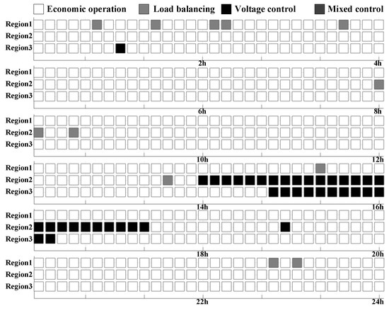
Figure 7.
Three regions with 24 h operational control modes.
Figure 8, Figure 9 and Figure 10 present the results of node voltage, load, and network losses over a day under different operating scenarios. As shown in these figures, compared with Scenario I, the proposed method effectively maintains voltage levels by adjusting the reactive power output of DG inverters in Scenario II, thereby improving voltage profiles, reducing load imbalances, and enhancing overall system performance.
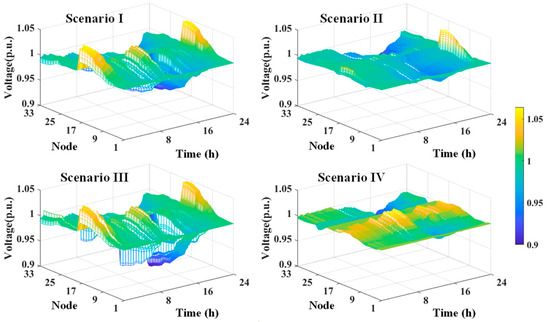
Figure 8.
24 h node voltage profiles in the four scenarios.
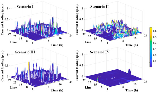
Figure 9.
24 h current loading in the four scenarios.
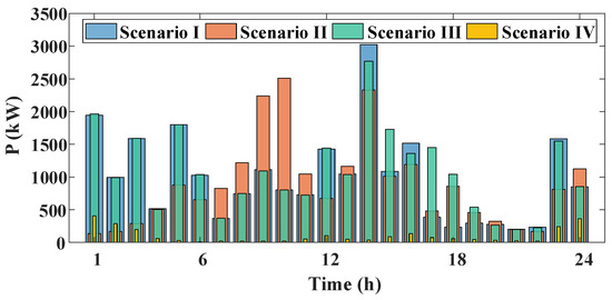
Figure 10.
24 h network loss in the four scenarios.
To measure the impact of control, the voltage deviation index () and load balance index () are outlined as follows:
where is the node index, denotes the number of nodes in distribution network, is the voltage measurement of node at time , is the branch index, is the total number of branches in the distribution network, and is the equivalent load measurement of branch at time .
The outcomes of control for the four scenarios are displayed in Table 4. Compared with Scenario I, the data-driven multi-region coordinated control in Scenario II significantly reduces voltage fluctuations and load imbalances, achieving reductions of 31.25%, 19.17%, and 20.68% in voltage deviation, load imbalance, and power loss, respectively. Note that, network losses are calculated from the difference between injected and consumed power and can be validated through branch current and line resistance data when available. Compared with Scenario III, Scenario II also shows better voltage regulation, mainly because information exchange between regions enables faster convergence under the same three control iterations. However, relative to Scenario IV, Scenarios I–III perform worse in optimizing these indicators, since Scenario IV is a model-based method with precise physical parameters, representing the theoretical optimum, which are often unavailable in practice.
Table 4.
Results of four scenarios.
Figure 11 illustrates the reactive power output of DGs over 24 h. The proposed method enables rapid adjustment of DG inverter reactive power to mitigate frequent voltage fluctuations caused by high DG penetration. From 0:00 to 8:00 in Region 3, substantial DG active power output causes the voltage to exceed the upper limit, prompting inverters to primarily absorb reactive power to reduce it. In Region 2, where load demand is higher, inverters supply additional reactive power to maintain voltage levels. Between 13:00 and 17:00, as load demand in Region 3 increases, inverters again supply reactive power accordingly. These findings confirm that the proposed method flexibly regulates DG outputs, effectively reducing voltage deviations.
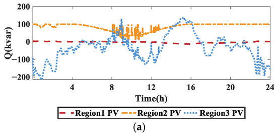
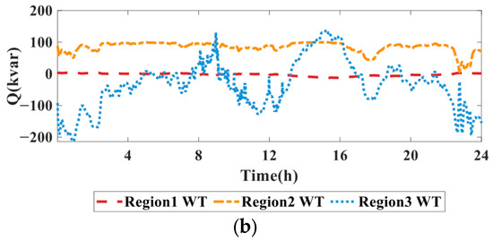
Figure 11.
24 h DGs reactive power outputs. (a) PVs; (b) WTs.
3.3. Computational Efficiency Analysis
The proposed data-driven method requires continuous interaction with the distribution network, which inevitably affects its operation. Therefore, it is crucial for this approach to achieve fast convergence within several iterations to minimize its impact on the network’s operation. In this analysis, the test is conducted under the source-load state at 10:00, and the iteration process terminates when the residual reaches the predefined convergence threshold of 0.001. The voltage iteration process, residual iteration process, and DG output iteration process are depicted in Figure 12, Figure 13 and Figure 14, respectively. As shown, the proposed data-driven multi-region coordinated control method achieves rapid convergence within only 6 iterations through regional coordination, significantly outperforming the centralized data-driven method, which requires 15 iterations.
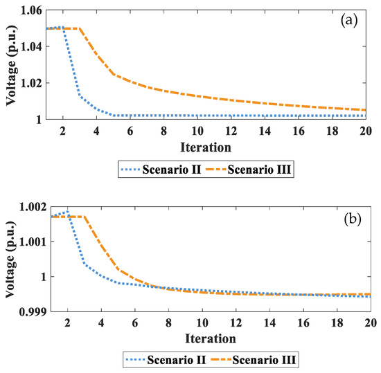
Figure 12.
Comparison of voltage iteration process. (a) Node 18; (b) Node 25.
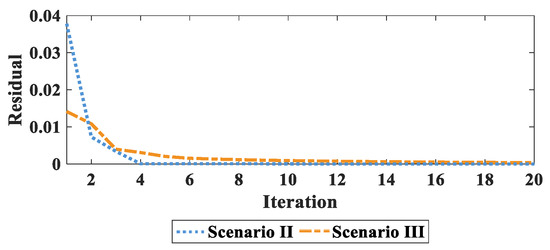
Figure 13.
Residual iteration process.
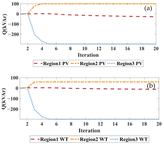
Figure 14.
DG output iteration process. (a) PVs; (b) WTs.
The computational efficiency and communication burden results are presented in Table 5. The proposed distributed data-driven method achieves a per-step computational time of only 0.0642 s, which is well below the control interval of 20 s. Compared with the centralized data-driven method, which requires 0.1569 s per step, the proposed method reduces the computation time by approximately 1.4-fold. In addition, to quantify the communication burden, the total data exchanged per controller in one control cycle is reported. The proposed method requires only 2.1 KB, compared with 7.7 KB for the centralized approach, demonstrating a clear advantage in reducing communication overhead. Overall, compared with the centralized approach, the distributed strategy significantly decreases both computational time and communication demand, achieving an overall computational speed improvement of more than five-fold and highlighting its strong potential for real-time operation.
Table 5.
Comparison of computational efficiency and communication burden.
3.4. Robustness Analysis
3.4.1. Robustness to Measurement Errors
The robustness of the proposed method is demonstrated in the presence of measurement errors. Voltage measurement deviations are set within ±0%, ±0.05%, ±0.5%, ±1%, ±2%, and ±3%, and the proposed method is applied for control. The voltage at Node 18 under different measurement errors is shown in Figure 15, and the specific indicators of voltage control performance are summarized in Table 6.
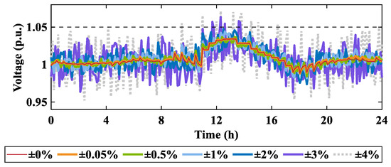
Figure 15.
Voltage control performance at node 18 under different measurement errors.
Table 6.
Comparison of voltage control performance under different measurement errors.
As shown in Figure 15 and Table 6, when the measurement error is less than ±1%, the voltage control performance is almost identical to that under error-free conditions. As the error increases to ±2%, voltage fluctuations slightly increase but remain better than the initial operating state in Scenario I. However, when the error exceeds ±3%, voltage fluctuations rise sharply and even surpass the upper voltage limit of 1.05 p.u. This is because a ±3% error already accounts for a considerable portion of the allowable operating voltage range (±10%) in distribution networks. Therefore, the proposed method is insensitive to small measurement errors (≤±2%), but when the error exceeds this threshold, the control performance deteriorates rapidly and may even worsen the operating state of the distribution network.
It should be noted that, in practical power systems, the measurement accuracy is much higher than the range considered in this study. The magnitude error of phasor measurement units (PMUs) is typically as low as 0.1–0.5%, while that of supervisory control and data acquisition (SCADA) systems is generally around 1% [37]. For larger measurement errors, techniques such as online identification [36] can be applied. Therefore, the proposed method has considerable practical value in real-world applications.
3.4.2. Adaptability to Voltage Sudden Changes
The stochastic nature of DGs may lead to sudden voltage rises or drops in distribution networks. This section verifies the adaptability of the proposed method under voltage disturbances. At 12:00, two operating states are defined: State 1 and State 2. In State 1, the active power output of the PV in Area 3 is 100%, while in State 2 it is 0%. The transition from State 1 to State 2 represents a sudden reduction in PV output, thereby testing the adaptability of the proposed method. In addition, different values of the parameter in (25) are selected to analyze their influence on control performance.
The voltage variation process is shown in Figure 16.
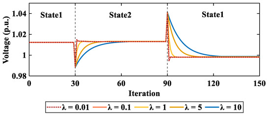
Figure 16.
Adaptability to voltage sudden changes under different values of .
As shown in Figure 16, at the 30th and 90th iterations, the system switches between State 1 and State 2, and the sudden change in PV output causes voltage fluctuations. When , the proposed method restores the voltage to around 1.0 within a single iteration, with a computation time of approximately 0.0642 s per iteration, indicating that the method can quickly restore the voltage level. Moreover, the parameter has a significant impact on convergence characteristics: larger values result in slower convergence and smoother voltage adjustments, while smaller values lead to faster convergence but may cause overshoot. When the adjustable capacity of devices is sufficient, an excessively small may induce large overshoot and system oscillations. Therefore, in practical applications, it is recommended to initially adopt a relatively large and then adjust it gradually according to the actual control performance.
3.5. Scalability Analysis
To verify the scalability of the proposed method, the modified IEEE 123-node distribution network is adopted. The system topology and regional partitioning adopt the results from [38] and are shown in Figure 17. Twelve DG units are integrated into the system, and their types, locations, and capacities are detailed in Table 7. All DG inverters are equipped with reactive power compensation functions. The network is partitioned into four regions: Region 1 (commercial), Region 2 (industrial), and Regions 3 and 4 (residential). The total active and reactive power demands of the system are 3.49 MW and 1.92 Mvar, respectively. The Scenarios I and II in Section 3.1 are also carried out in the test case.
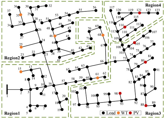
Figure 17.
Modified IEEE 123-node distribution network topology and partitioning.
Table 7.
Location, type and capacity of DGs.
The control performance of Scenario I and II in the large-scale system is presented in Table 8. Compared with Scenario I, the proposed method in Scenario II reduces voltage deviation, load imbalance, and power loss by 36.06%, 50.79%, and 51.18%, respectively, demonstrating its ability to maintain satisfactory control performance in large-scale, multi-region distribution networks.
Table 8.
Control performances of the IEEE 123-node system.
The computational efficiency and communication burden for the 123-node system are summarized in Table 9. In multi-region coordinated data-driven control problems, the computational time increases approximately linearly with the number of network nodes. Nevertheless, the per-iteration computational time remains well below the 20 s control step set in this study, confirming the feasibility of implementing the proposed method in practical large-scale distribution networks.
Table 9.
Computational efficiency of control process.
In summary, the scalability analysis demonstrates that the proposed data-driven multi-mode control method remains effective in large-scale active distribution networks. By leveraging regional partitioning and parallelized computation, the method effectively balances computational complexity and communication burden, thereby ensuring its practicality and applicability to real-world large-scale systems.
4. Conclusions
This paper proposes a distributed data-driven multi-mode control method for distribution networks to address the challenges of frequent DG fluctuations. A dynamic linearization approach is used to construct regional data models, enabling each region to adaptively select appropriate operating modes. A distributed gradient descent algorithm is applied to iteratively solve regional DG control strategies and directly implement them in the network, enabling rapid responses to DG variations. Case studies on the modified IEEE 33-node and 123-node test systems demonstrate that the proposed method outperforms centralized data-driven control, providing faster responses to DG fluctuations and achieving performance comparable to model-based approaches. By regulating DG reactive power, the method reduces voltage deviation, load imbalance, and power loss by 31.25%, 19.17%, and 20.68%, respectively. In addition, the proposed method shows strong robustness against measurement errors and effectively adapts to sudden voltage changes.
Several critical issues are worth further research. The protection of data privacy in inter-regional coordination can be further incorporated to ensure secure and reliable information exchange. In addition, the integration of physical models with measurement data can be investigated, utilizing physical knowledge to refine the modal mapping matrix of data models, thereby improving control performance. Moreover, it is significant to consider transient behaviors and the impacts of harmonics on distribution network operation to enhance the safety and reliability of practical applications.
Author Contributions
Conceptualization, Y.Z.; methodology, H.Z.; validation, Z.L.; formal analysis, S.G.; resources, H.J.; writing, Q.Y. All authors have read and agreed to the published version of the manuscript.
Funding
This research was supported by the Guizhou Provincial Science and Technology Project under Grant [2023] General 292, and by the Science and Technology Project of Guizhou Power Grid under Grant 060000KC24010012.
Data Availability Statement
The original contributions presented in the study are included in the article. Further inquiries can be directed to the corresponding author.
Conflicts of Interest
Authors Youzhuo Zheng, Hengrong Zhang and Zhi Long are employees of the Electric Power Research Institute, Guizhou Power Grid Co., Ltd. (Guiyang, China); The remaining authors declare that the research was conducted in the absence of any commercial or financial relationships that could be construed as a potential conflict of interest.
Appendix A
In the control process of distribution networks, coordination among adjacent regions is ensured by defining equivalent control measurements, as expressed in Equation (5), thereby achieving multi-region consistency. This section provides a theoretical analysis of the convergence consistency of the data-driven models for each region. For simplicity, the mode flag is omitted from the mode mapping matrices in the following expressions.
To prove convergence consistency, the following theorem is stated:
Theorem A1.
If the target distribution network satisfies Assumptions 1 and 2, then there exists a parameter such that for any region with , , , and , convergence consistency can be achieved across all regions.
Proof of Theorem.
The boundedness of the mode mapping matrix
is proven first.
If Equation (24) holds, then is bounded. The mode mapping matrix estimation error is defined as . Then, Equation (23) becomes:
Define and , where and (). Equation (A1) further becomes:
Since is bounded, each term of is also bounded. Assuming , substituting this into Equation (A2) on both sides yields:
Squaring both sides of the equation results in:
Given and , it follows that:
Then there must exist a constant such that:
Furthermore, Equation (A3) can be expressed as:
Thus, is bounded, and consequently, is also bounded. Since is bounded, must also be bounded.
Next, the convergence of the equivalent control measurements in each region is proven.
Considering the dynamic linearization model (2) and the iterative process (25), the following equation is obtained:
There exists such that when , the following equation holds:
Substituting Equation (A9) into Equation (A8) results in:
where , . Since each part of is bounded and , it follows that , where .
Equation (A10) can be further simplified to:
This completes the proof that the equivalent control measurements in each region are bounded.
The proof of Theorem 1 is complete. □
The consistency convergence of different regions ensures the effective implementation of the data-driven multi-region coordinated control method.
References
- Luo, Y.; Tian, P.; Yan, X.; Xiao, X.; Ci, S.; Zhou, Q.; Yang, Y. Energy Storage Dynamic Configuration of Active Distribution Networks-Joint Planning of Grid Structures. Processes 2024, 12, 79. [Google Scholar] [CrossRef]
- Zhang, Z.; Liu, L.; Cai, Y.; Peng, Z.; Shi, L.; Li, X. Analysis of Line Loss Change Trend of Large-scale New Energy Access Distribution Network Under New Power System. Power Syst. Big Data 2024, 27, 11–22. (In Chinese) [Google Scholar] [CrossRef]
- Haider, R.; Annaswamy, A.M. A Hybrid Architecture for Volt-Var Control in Active Distribution Grids. Appl. Energy 2022, 312, 118735. [Google Scholar] [CrossRef]
- Yao, Q.; Li, X. Active-reactive Power Coordinated Optimization Control Method of Rural Power Distribution System with High Proportion of Distributed Resources. Power Syst. Big Data 2024, 27, 19–30. [Google Scholar] [CrossRef]
- Yuan, W.; Yuan, X.; Xu, L.; Zhang, C.; Ma, X. Harmonic Loss Analysis of Low-Voltage Distribution Network Integrated with Distributed Photovoltaic. Sustainability 2023, 15, 4334. [Google Scholar] [CrossRef]
- Zhang, Z.; Li, P.; Ji, H.; Yu, H.; Zhao, J.; Xi, W.; Wu, J. Adaptive Voltage Control of Inverter-Based DG in Active Distribution Networks with Measurement-Strategy Mapping Matrix. IEEE Trans. Sustain. Energy 2025, 16, 1238–1252. [Google Scholar] [CrossRef]
- Zhou, H.; Liang, J.; Du, X.; Wu, M. Multi-Timescale Reactive Power Optimization and Regulation Method for Distribution Networks Under a Multi-Source Interaction Environment. Processes 2024, 12, 2254. [Google Scholar] [CrossRef]
- Aboshady, F.M.; Pisica, I.; Zobaa, A.F.; Taylor, G.A.; Ceylan, O.; Ozdemir, A. Reactive Power Control of PV Inverters in Active Distribution Grids with High PV Penetration. IEEE Access 2023, 11, 81477–81496. [Google Scholar] [CrossRef]
- Zhang, C.; Xu, Y.; Dong, Z.; Ravishankar, J. Three-Stage Robust Inverter-Based Voltage/Var Control for Distribution Networks with High-Level PV. IEEE Trans. Smart Grid 2019, 10, 782–793. [Google Scholar] [CrossRef]
- Xu, R.; Zhang, C.; Xu, Y.; Dong, Z.; Zhang, R. Multi-Objective Hierarchically-Coordinated Volt/Var Control for Active Distribution Networks with Droop-Controlled PV Inverters. IEEE Trans. Smart Grid 2022, 13, 998–1011. [Google Scholar] [CrossRef]
- Jiao, W.; Chen, J.; Wu, Q.; Li, C.; Zhou, B.; Huang, S. Distributed Coordinated Voltage Control for Distribution Networks with DG and OLTC Based on MPC and Gradient Projection. IEEE Trans. Power Syst. 2022, 37, 680–690. [Google Scholar] [CrossRef]
- Li, P.; Ji, H.; Wang, C.; Zhao, J.; Song, G.; Ding, F.; Wu, J. Coordinated Control Method of Voltage and Reactive Power for Active Distribution Networks Based on Soft Open Point. IEEE Trans. Sustain. Energy 2017, 8, 1430–1442. [Google Scholar] [CrossRef]
- Bu, X.; Hou, Z.; Zhang, H. Data-Driven Multiagent Systems Consensus Tracking Using Model Free Adaptive Control. IEEE Trans. Neural Netw. Learn Syst. 2018, 29, 1514–1524. [Google Scholar] [CrossRef]
- Babu, R.; Raj, S.; Bhattacharyya, B. Weak Bus-Constrained PMU Placement for Complete Observability of a Connected Power Network Considering Voltage Stability Indices. Prot. Control Mod. Power Syst. 2020, 5, 28. [Google Scholar] [CrossRef]
- Cheng, G.; Lin, Y.; Abur, A.; Gómez-Expósito, A.; Wu, W. A Survey of Power System State Estimation Using Multiple Data Sources: PMUs, SCADA, AMI, and Beyond. IEEE Trans. Smart Grid 2024, 15, 1129–1151. [Google Scholar] [CrossRef]
- Liang, X.; Fang, R.; Gan, Q.; Shi, L.; He, L.; Guan, C. Big Data Integration Technology and Application in Novel Power Distribution Network. Power Syst. Big Data 2022, 25, 53–61. (In Chinese) [Google Scholar] [CrossRef]
- Zhang, X.; Wu, Z.; Sun, Q.; Gu, W.; Zheng, S.; Zhao, J. Application and Progress of Artificial Intelligence Technology in the Field of Distribution Network Voltage Control: A Review. Renew. Sustain. Energy Rev. 2024, 192, 114282. [Google Scholar] [CrossRef]
- Huo, Y.; Li, P.; Ji, H.; Yu, H.; Yan, J.; Wu, J.; Wang, C. Data-Driven Coordinated Voltage Control Method of Distribution Networks with High DG Penetration. IEEE Trans. Power Syst. 2023, 38, 1543–1557. [Google Scholar] [CrossRef]
- Yuan, Z.; Cavraro, G.; Singh, M.K.; Cortés, J. Learning Provably Stable Local Volt/Var Controllers for Efficient Network Operation. IEEE Trans. Power Syst. 2024, 39, 2066–2079. [Google Scholar] [CrossRef]
- Sun, X.; Qiu, J.; Zhao, J. Optimal Local Volt/Var Control for Photovoltaic Inverters in Active Distribution Networks. IEEE Trans. Power Syst. 2021, 36, 5756–5766. [Google Scholar] [CrossRef]
- Liang, X.; Zhou, N.; Fang, R.; Gan, Q.; Jiang, Y.; Guan, C.; Shi, L. Bi-level Optimization for Integrated Energy System Considering Cloud-Edge Collaboration. Power Syst. Big Data 2023, 26, 9–17. (In Chinese) [Google Scholar] [CrossRef]
- Hossain, R.R.; Kumar, R. A Distributed-MPC Framework for Voltage Control Under Discrete Time-Wise Variable Generation/Load. IEEE Trans. Power Syst. 2024, 39, 809–820. [Google Scholar] [CrossRef]
- Wang, S.; Duan, J.; Shi, D.; Xu, C.; Li, H.; Diao, R.; Wang, Z. A Data-Driven Multi-Agent Autonomous Voltage Control Framework Using Deep Reinforcement Learning. IEEE Trans. Power Syst. 2020, 35, 4644–4654. [Google Scholar] [CrossRef]
- Kamruzzaman, M.; Duan, J.; Shi, D.; Benidris, M. A Deep Reinforcement Learning-Based Multi-Agent Framework to Enhance Power System Resilience Using Shunt Resources. IEEE Trans. Power Syst. 2021, 36, 5525–5536. [Google Scholar] [CrossRef]
- Wang, Y.; Vittal, V. Data Driven Real-Time Dynamic Voltage Control Using Decentralized Execution Multi-Agent Deep Reinforcement Learning. IEEE Open Access J. Power Energy 2024, 11, 508–519. [Google Scholar] [CrossRef]
- Zhang, M.; Guo, G.; Magnússon, S.; Pilawa-Podgurski, R.C.N.; Xu, Q. Data Driven Decentralized Control of Inverter Based Renewable Energy Sources Using Safe Guaranteed Multi-Agent Deep Reinforcement Learning. IEEE Trans. Sustain. Energy 2024, 15, 1288–1299. [Google Scholar] [CrossRef]
- Mi, B.; Huo, X.; Ma, K.; Jin, S. Dynamic Linearization Residual-Assisted Model-Free Adaptive Control with Modified Criterion Function Based on Extended FFDL Data Model. IEEE Trans. Ind. Electron. 2025, 75, 10585–10594. [Google Scholar] [CrossRef]
- Coutinho, P.H.S.; Bessa, I.; Peixoto, M.L.C.; Palhares, R.M. A co-design condition for dynamic event-triggered feedback linearization control. Syst. Control Lett. 2024, 183, 105678. [Google Scholar] [CrossRef]
- Bozza, A.; Martin, T.; Cavone, G.; Carli, R.; Dotoli, M.; Allgöwer, F. Online Data-Driven Control of Nonlinear Systems Using Semidefinite Programming. IEEE Control Syst. Lett. 2024, 8, 3189–3194. [Google Scholar] [CrossRef]
- Clelland, J.N.; Klotz, T.J.; Vassiliou, P.J. Dynamic Feedback Linearization of Control Systems with Symmetry. SIGMA 2024, 20, 058. [Google Scholar] [CrossRef]
- Da Cunha, S.B. On the robustness of feedback linearization. Int. J. Dyn. Control 2024, 12, 3318–3331. [Google Scholar] [CrossRef]
- Hou, Z.; Xiong, S. On Model-Free Adaptive Control and Its Stability Analysis. IEEE Trans. Autom. Control 2019, 64, 4555–4569. [Google Scholar] [CrossRef]
- Guo, Y.; Hou, Z.; Liu, S.; Jin, S. Data-Driven Model-Free Adaptive Predictive Control for a Class of MIMO Nonlinear Discrete-Time Systems with Stability Analysis. IEEE Access 2019, 7, 102852–102866. [Google Scholar] [CrossRef]
- Wu, X.; Wang, M.; Shahidehpour, M.; Feng, S.; Chen, X. Model-Free Adaptive Control of STATCOM for SSO Mitigation in DFIG-Based Wind Farm. IEEE Trans. Power Syst. 2021, 36, 5282–5293. [Google Scholar] [CrossRef]
- Gao, S.; Li, P.; Ji, H.; Zhao, J.; Yu, H.; Wu, J.; Wang, C. Data-driven Multi-mode Adaptive Operation of Soft Open Point with Measuring Bad Data. IEEE Trans. Power Syst. 2024, 39, 6482–6495. [Google Scholar] [CrossRef]
- Song, G.; Yu, C.; Ji, H.; Zhao, J.; Xu, J.; Li, P. Data-Driven Voltage Control of Energy Storage Integrated Soft Open Point Considering Quality of Measurement Data. Autom. Electr. Power Syst. 2023, 47, 90–100. (In Chinese) [Google Scholar]
- Sun, J.; Chen, Q.; Xia, M. Data-Driven Detection and Identification of Line Parameters with PMU and Unsynchronized SCADA Measurements in Distribution Grids. CSEE J. Power Energy Syst. 2024, 10, 261–271. [Google Scholar] [CrossRef]
- Chai, Y.; Guo, L.; Wang, C.; Zhao, Z.; Du, X.; Pan, J. Network Partition and Voltage Coordination Control for Distribution Networks with High Penetration of Distributed PV Units. IEEE Trans. Power Syst. 2018, 33, 3396–3407. [Google Scholar] [CrossRef]


Disclaimer/Publisher’s Note: The statements, opinions and data contained in all publications are solely those of the individual author(s) and contributor(s) and not of MDPI and/or the editor(s). MDPI and/or the editor(s) disclaim responsibility for any injury to people or property resulting from any ideas, methods, instructions or products referred to in the content. |
© 2025 by the authors. Licensee MDPI, Basel, Switzerland. This article is an open access article distributed under the terms and conditions of the Creative Commons Attribution (CC BY) license (https://creativecommons.org/licenses/by/4.0/).