Article

Prediction of Influencing Factors on Estimated Ultimate Recovery of Deep Coalbed Methane: A Case Study of the Daning–Jixian Block

1
PetroChina Coalbed Methane Company Limited, Beijing 100028, China
2
China United Coalbed Methane National Engineering Research Center Co., Ltd., Beijing 100095, China
3
Sanya Offshore Oil & Gas Research Institute, Northeast Petroleum University, Sanya 572025, China
*
Author to whom correspondence should be addressed.
Processes 2025, 13(1), 31; https://doi.org/10.3390/pr13010031
Submission received: 21 November 2024 / Revised: 17 December 2024 / Accepted: 21 December 2024 / Published: 26 December 2024

Abstract

:
China has vast amounts of deep coalbed methane resources but is still in the early stage of deep coalbed methane development; thus, it lacks mature gas exploitation and development theories and technologies, particularly effective methods for evaluating final recoverable reserves. This paper intends to develop a method that can rapidly and accurately predict deep coalbed methane EUR before well spacing to guide the formulation of rational exploitation schemes and full exploitation of geological resources, thus lowering costs and enhancing efficiency. Taking deep coalbed methane in the Daning–Jixian block of the Ordos Basin as the research object, this paper first uses the production decline method to evaluate the EUR of brought-in wells and analyzes the influence of geological conditions and engineering parameters on the EUR. Second, the ADASYN method is used to process the unevenly distributed samples to solve the small number and poor representativeness of the machine learning model samples. After this, the BP neural network, support vector machine, and Gaussian process regression are used to build EUR evaluation models, and the models are compared and the best is selected. Lastly, the selected EUR evaluation model is applied to analyze the influence weights of geological conditions and engineering parameters on EUR. According to the research results, the MAPEs of the BP neural network, support vector machine, and Gaussian process regression models reach 7.03%, 7.23%, and 1.28%, respectively, after ADASYNA oversampling. However, the Gaussian process regression model may bear the risk of overfitting. The model comparison results show that the support vector machine model is superior to the BP neural network model and the Gaussian process regression model. Therefore, the support vector machine is favorably selected to predict EUR in this paper. Feature importance analysis results indicate that engineering parameters (including clusters, horizontal length, fracturing liquid, and proppant) are the major factors influencing the EUR prediction results. This paper establishes a model for predicting the EUR of deep coalbed methane, which provides a reference for the future formulation of well spacing schemes in the surveyed region.

1. Introduction

Coalbed methane constitutes a major part of unconventional natural gas, and China has abundant coalbed methane resources [1]. Notably, China possesses a huge quantity of deep coalbed methane resources, with 18.4–40.71 trillion cubic meters of deep coalbed methane buried at a depth of 2000 m or deeper [2,3,4,5]. China is moving to an era of synchronously boosting deep coalbed methane in various regions. Breakthroughs have been successfully made in the production of deep coalbed methane wells in large basins such as Ordos Basin, Sichuan Basin, and Junggar Basin [6,7,8,9,10,11]. In 2021, ultra-scale limited fracturing was tested on Jishen 6-7 Horizontal Well No. 01 of the Daning–Jixian Block on the eastern edge of the Ordos Basin, with a vertical depth of 2200 m and a horizontal length of 1000 m; daily gas production of over 100,000 cubic meters was achieved [4]. This horizontal well is the first coalbed methane well in China to exceed daily gas production of over 100,000 cubic meters, marking the start of large-scale development of deep coalbed methane in China.
China is at the very beginning of deep coalbed methane development, and its methane exploitation and development theories and technologies are underdeveloped. For example, China has not yet developed a mature estimated ultimate recovery (EUR) evaluation method [12]. EUR is one of the critical evaluation indexes for predicting the results of deep coalbed methane development. If the EUR can be determined for different well spacing schemes before well spacing according to some geological conditions (such as the horizontal well length, the fracturing fluid amount, and proppant amount, etc.), high-cost exploitation activities in areas with low gas production potential can be avoided, and the formulation of well layout schemes can be guided to maximize the yields and benefits of methane exploitation. Therefore, the accuracy of EUR prediction before well spacing can determine whether one can develop rational exploitation schemes, fully exploit geological resources, and attain the goal of lowering costs and improving efficiency [13].
Under different geological conditions, the choice of well placement and development will result in varying production capacities that correspond to different costs and, consequently, affect development efficiency. To optimize development from an integrated geological–engineering perspective and achieve maximum development efficiency, it is essential to accurately evaluate the potential production capacity and associated costs for different development schemes. Accurate evaluation of production capacity is the key and challenging aspect of this work. It is necessary to determine the potential production capacity under different geological conditions and with various combinations of development plans. Therefore, a method needs to be developed to effectively predict EUR based on geological conditions and engineering parameters, even in regions with limited well data and low development levels, providing a theoretical basis for further well placement.
In oil and gas resource development, accurately predicting the EUR is of great significance. Although existing decline models are widely applied for long-term production forecasting based on production data, deep coalbed methane development requires a method capable of quickly and accurately evaluating EUR before drilling to provide a scientific basis for the formulation and optimization of development plans. As EUR has great significance for guiding the exploitation and development of oil and gas resources, Chinese and foreign scholars have developed some EUR evaluation methods, among which the production decline method is the most widely used in oil fields [14,15]. This method can predict the EUR mainly according to the decline law for oil and gas production data. J.J. Arps first summarized three production decline laws for oil and gas fields in 1945—exponential decline, hyperbolic decline, and harmonic decline [16,17]—and his decline theory was widely used in oil fields. Based on Arps’ production decline theory, Chinese and foreign scholars improved or reconstructed the oil and gas production decline characteristics of different reservoirs, such as tight sandstone [18,19] and shale [20,21]. The prerequisite for successfully applying the production decline method is that long-term, stable historical production data are acquired, and it is difficult to evaluate the EUR before well spacing. It is urgent to develop a method that can quickly and accurately predict EUR before well spacing of deep coalbed methane to guide the formulation and optimization of methane exploitation schemes.
In recent years, machine learning methods, with their ability to efficiently capture nonlinear relationships, have shown great potential in EUR prediction for coalbed methane and have achieved promising initial results. This method can skillfully capture complex nonlinear mapping relationships without building complex mechanism models. Additionally, it has high evaluation accuracy and low calculation costs, so it has been successfully applied in oil exploitation and development fields such as geochemical parameter logging evaluation [22], physical property parameter logging evaluation of reservoirs [23], and seismic property interpretation [24]. Some scholars have recently used machine learning to predict the EUR of coalbed methane and found that machine learning has high application potential in this field. Feng Kun et al. [25] used a stochastic forest algorithm optimized by the genetic algorithm to predict the production of deep coalbed methane. Zhu Qingzhong et al. [26] analyzed the drainage and exploitation parameters of coalbed methane wells in Zhengcun and Zhengzhuang blocks in the Qinshui Basin and applied machine learning methods such as stochastic forest and neural networks to predict the production of coalbed methane wells. Song Hongqing et al. [27] built support vector machine regression and stochastic forest models to predict the production of the single coalbed methane well in Qinshui Basin, Shanxi Province. The above studies indicate that machine learning plays a major role in predicting the EUR of deep coalbed methane.
Given that deep coalbed methane exploration and development are still in their infancy, with limited well data and imbalanced data distribution, this study employs the ADASYN algorithm to balance minority EUR samples, thereby improving the prediction accuracy and generalization ability of the machine learning models. As mentioned above, the exploitation and development of deep coalbed methane is still in its initial stage in China. Even in the Daning–Jixian block, which made the first breakthrough in this aspect, the number of wells that can be EUR evaluation modeling wells (which can be evaluated by the production decline method and have known geological conditions and engineering parameters) is quite limited due to the small number of brought-in wells. Worse still, the number of wells with low and high EUR values is limited, so the distribution is not even. As the machine learning algorithm is driven by data, the unbalanced data distribution will seriously reduce the prediction accuracy and generalization ability of the training model. To solve the data imbalance problem, Chawla [28] developed the SMOTE algorithm to synthesize new samples according to the data characteristics of minority samples to increase the number of minority-class samples to ameliorate data imbalance in the machine learning process. Haibo He [29] proposed the ADASYN algorithm based on the SMOTE algorithm. Compared with the SMOTE algorithm, the ADASYN algorithm can process minority-class data samples with different densities and distributions more flexibly, generate representative samples more effectively, and reduce redundancy and noise. In this paper, the ADASYN algorithm is used to solve the data imbalance problem associated with minority-class EUR samples.
This paper takes deep coalbed methane in the Daning–Jixian block of Ordos Basin as the research object. First of all, this paper adopts the production decline method to evaluate the EUR of brought-in wells and analyzes the influence of geological conditions and engineering parameters on EUR. Second, to avoid the small size and unbalanced distribution of samples in machine learning modeling, the ADASYN algorithm is used to solve sample imbalance. After that, this paper establishes several EUR evaluation models using some machine learning methods, compares the models, and eventually selects one. Lastly, the influence weights of geological conditions and engineering parameters on EUR prediction results are analyzed. The deep coalbed methane EUR prediction model built for the limited number of brought-in wells in this paper will provide some reference for further optimization of well spacing schemes in the survey region.

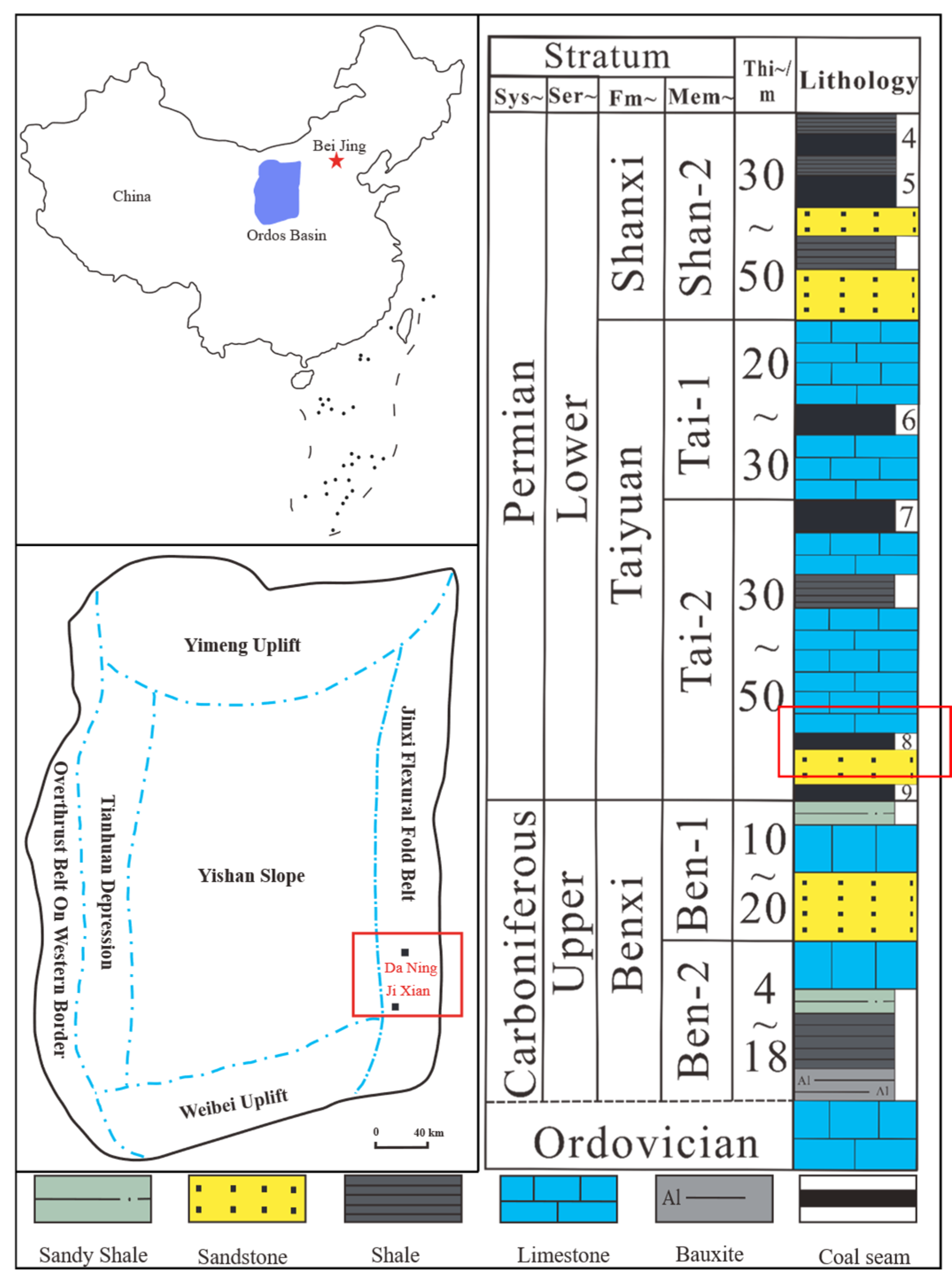
2. Geological Conditions of the Survey Region

The Ordos Basin, an important coal-bearing basin in China, covers an area of about 25 × 104 km2, spans the five provinces of Shanxi and Mongolia, Shaanxi, Gansu, and Ningxia, and borders Hetao, Yinchuan, Liupanshan, and Weihe basins. Based on the crystallization of Archean and Proterozoic eon, the basin developed from a marginal Marine basin into a large cratonic basin (the present basin shape) under the influence of the Indosinian, Yanshanian, and Himalayan tectonic movements from early Paleozoic to late Mesozoic periods. The southeast margin of the basin is currently a hot area for coalbed methane development [6].
The Daning–jixian block is located in the southeast margin of the Ordos Basin, mainly developed in the No. 8 coal seam of the Carboniferous Taiyuan Formation and the No. 5 coal seam of the Permian Shanxi Formation (Figure 1). The survey region is the No. 8 coal seam of the Taiyuan Formation, which is the primary target layer for deep coalbed methane exploration, with a gently-dipping monoclinic structure in the NW direction, undeveloped faults, a buried depth range of 1800–2520 m, a thickness range of 5.0 to 12.0 m, and an average thickness of 7.6 m [30].

3. Research Methodology

The research workflow for this study (Figure 2) is as follows: First, the EUR of production wells is evaluated using the production decline method, and the ADASYN algorithm is applied to address data imbalance issues. Subsequently, models are constructed and compared using BPNN, SVR, and GPR to select the optimal prediction model. Finally, feature importance analysis is conducted to identify the key factors influencing EUR, providing a scientific basis for the development of deep coalbed methane.

3.1. Production Decline Method

The production decline method is a prediction method developed based on the phenomenon that the production of oil and gas wells drops progressively with time [31,32]; specifically, this method uses mathematical models to predict the future production of wells based on the production performance of oil and gas wells to evaluate the final recoverable oil and gas reservoirs. Different decline models apply to corresponding production conditions and reservoir characteristics. Table 1 lists the existing commonly used production decline method models.
The coalbed methane production decline law is complex and regions may vary in the production decline law [36]. In the Daning–Jixian block, deep coalbed methane wells have characteristics of gas production immediately after going into operation, high production in the initial stage, high decline rate, and slow decline of gas production in the later period [37]. Li Mingzhai et al. [38] (2024) analyzed the coalbed methane production decline law in the Daning–Jixian block and found that its methane production law is similar to that of shale gas wells, presenting a “hyperbolic + exponential” production decline law. Overall, the deep coalbed methane wells mainly produce free gas and show the hyperbolic production decline law in the early production stage and the wells produce absorbed gas as the main and free gas as the second and follow the exponential decline law in the middle and later production stages. This paper adopts two production decline models: the hyperbolic decline model for the early production stage and the exponential decline model for the second stage when the decline rate is lower than 20%.

3.2. Machine Learning Algorithms

The core of machine learning is to use computers to discover potential rules from massive complex data and utilize the rules to predict future events and trends [39]. Machine learning covers a variety of algorithms, such as linear models, decision trees, neural networks, support vector machine regression, integration methods, clustering algorithms, and deep learning.
Linear regression (LR), support vector regression (SVR), back propagation neural network (BPNN), Gaussian process regression (GPR), and other algorithms have been widely applied in oil and gas production prediction [10].
This paper combines geological and engineering factors to predict deep coalbed methane production. It selects and uses eight parameters, including coal-seam thickness, gas content, porosity, permeability, horizontal length, the total number of clusters, the amount of fracturing liquid, and proppants as input parameters, takes EUR as the output parameter, and adopts three machine learning algorithms, BP neural network, support vector machine, and Gaussian process regression to predict EUR.

3.2.1. BP Neural Network

The BP neural network algorithm was first proposed by Rumelhart and McClelland in 1986, designed to train the feedforward neural network of multi-layer perceptron through error using the backpropagation algorithm [40].
BP neural network is a typical multi-layer feedforward neural network. It usually consists of an input layer, one or more hidden layers, and an output layer, with the input layer receiving data, the hidden layer using the activation function to realize nonlinear transformation, and the output layer generating the final prediction result. Its core mechanism is to train the network using the backpropagation algorithm. The weights and bias parameters in the network are adjusted by comparing the errors between the model output and the target output. When used to process large-scale and high-dimensional data and deal with complex nonlinear relationships between input variables, BP neural networks can guarantee higher prediction accuracy. Therefore, the BP neural network is favored due to its simple mechanism, convenient operation, and wide application scope [41].

3.2.2. Support Vector Machine Regression

Support vector machine regression (SVR) is a machine learning algorithm proposed by Vapnik et al. in the 1990s [42]. It has been extended to solve complex linear inseparability and “dimensional disaster” of data. The core of SVR is to use the kernel function to map the sample data to a corresponding high-dimensional feature space to realize a nonlinear analysis of the original data and determine the optimal hyperplane according to mathematical derivation. Kernel function is the key parameter of SVR, with different degrees of sensitivity to different data categories. Typical kernel methods include linear kernel, polynomial kernel, Sigmoid kernel, and RBF kernel. This paper uses the RBF kernel function [43] as the kernel function of the SVR algorithm.
K ( x , x ) = e x p γ x x 2
where x and x represent the input sample, x x 2 denotes the Euclidean distance between the samples, and γ is an adjustable parameter that controls the width of the kernel function.
The core idea of the RBF kernel is to map data points in the input space to a high-dimensional feature space to better separate and fit the data points in the high-dimensional space. The RBF kernel has a local response, which indicates that it has a larger influence on samples closer to the target point and a smaller influence on samples farther away from the target point. Therefore, the RBF kernel has excellent performance in handling complex nonlinear relationships.

3.2.3. Gaussian Process Regression

Gaussian process regression (GPR) is a machine learning training method developed based on strict statistical principles and is extensively applied to solve regression and classification problems [44]. As GPR does not depend on a specific function type, it can be applied to handle a variety of complex data distributions and relationships and describes the correlation between data and its uncertainty well.
The main advantage of GPR lies in its ability to handle nonlinear relationships and small data sets. The regression features are mainly determined by the selection of the mean function and covariance function, so the model shows a high degree of flexibility and adaptability in capturing data features.
The GPR random variable f(x) is uniquely determined by its mean function m(x) and covariance function k(x, x′), and the Gaussian process is expressed as in [45]:
f ( x ) = GPR ( m ( x ) , k ( x , x ) ) m ( x ) = E ( f ( x ) ) k ( x , x ) = E ( f ( x ) m ( x ) ( f ( x ) m ( x ) ) )
where x and x′ are the input samples, E represents the mean operator, and GPR(·) denotes the Gaussian process distribution in function space.

3.3. Oversampling Algorithm

Due to the unbalanced data distribution, traditional machine learning algorithms have limitations in processing unevenly distributed data [46,47,48]. As oversampling has low algorithm complexity and strong generalization, it has been most commonly used in processing unbalanced data. Common oversampling methods include SMOTE and improved SMOTE methods.
Because the traditional SMOTE method has randomness in generating new synthetic samples, it may cause aliasing of samples. Scholars have developed some improved methods based on SMOTE. He et al. [29] proposed an Adaptive SMOTE algorithm, namely, Adaptive Synthetic (ADASYN) Oversampling, which can control the distribution of synthesized minority-class samples according to the sample distribution of the data set.
The basic approach of the ADASYN algorithm is to evaluate the concentration degree of majority-class samples around each minority-class sample according to the neighborhood structure of the minority-class sample to eventually determine the number of synthetic samples. Synthetic samples are generated according to the characteristics of minority-class samples to enhance the learning effect of the model.
The specific process of the ADASYN algorithm is as follows [29]:
Calculate the number of minority-class samples n min and majority-class samples n maj to determine the number of synthetic samples G. G can be expressed as follows:
G = n maj     n min
Use the K-nearest neighbor algorithm to search (k)-nearest neighbor samples in the whole data set for each minority-class sample x i , count up the number of majority-class samples in these neighbors, and calculate the proportion r i of majority-class samples using the following formula.
r i = k maj k
r i represents the proportion of the majority-class samples in the minority-class samples. The weight G i of the generated synthesized sample can be calculated as follows:
G i = r i j = 1 n m i n r j G
where j = 1 n min r j is the sum of the proportion of all minority-class samples. G i denotes the number of synthetic samples generated for each minority-class sample.
Generate new synthetic samples according to weights. Use the random interpolation method to generate a new sample for each minority-class sample x i . Specifically, a sample is randomly selected from the (k)-nearest neighbor samples of x i and a new sample is generated by the following formula:
x new = x i + λ x near x i
where λ is a random number in the range [0, 1]. The synthetic sample x new generated by this linear interpolation will fall between the minority-class sample x i and its neighbors, which can guarantee the diversity and representativeness of the generated samples.

3.4. Feature Importance Ranking Algorithms

The feature importance ranking algorithm can be used to calculate the dependence of the model on different feature parameters, so this can improve the explanatory power of the model, reduce the dimension of the model by screening key feature parameters, improve computational efficiency, and lower the risk of overfitting.
Feature importance ranking algorithms mainly include model-based algorithms [49], statistical feature selection-based algorithms [50], and feature change-based models [51]. This paper selects and uses a feature change-based algorithm, the Permutation Feature Importance (PFI) algorithm. This algorithm evaluates the actual contribution of a feature to the model by randomly replacing the value of a feature parameter and observing the change in the model’s prediction performance. The specific process is as follows [52]:
(1)
Calculate the baseline performance: Train the model on the original data set and calculate the performance indexes of the model (such as mean absolute percentage error, mean square error, etc.). The performance index is set as Porig.
Let the forecasting performance of the model on the original data be Porig = f(X,y). Where X is the input feature matrix, including the features of all samples, and y is the target variable (the actual value).
(2)
Permutate features: Permutate the data-concentrated feature Xj. In other words, disrupt the column data of the feature to mess up its relations with the target variable. Eventually, generate the new data set X j p e r m .
(3)
Calculate after-permutation performance: recalculate the performance of the model on the after-permutation data set X j p e r m and compute the performance index Pperm(Xj) using the following formula:
P p e r m X j = f ( X j p e r m , y )
(4)
Calculate the importance of features: the importance of the feature Xj is measured by the performance loss (that is, the quantity of performance change).
I m p o r t a n c e X j = P o r i g P o r i g ( X j )
A greater loss indicates greater importance of the feature because disrupting the value of the feature will more seriously hurt the model’s predictive power.
(5)
Repeat the permutation process: Repeat the above permutation process several times to acquire more stable and reliable feature importance. Calculate the performance loss of each permutation and then take its average value.
I m p o r t a n c e X j = 1 k i = 1 k P o r i g     P p e r m i ( X j )
where k is the number of permutations.

4. Results and Discussion

4.1. Analysis of EUR Influencing Factors

The initial production rate and decline rate are determined according to the historical production data of oil and gas wells. The stage-based decline model is applied to evaluate the EUR of each brought-in well. A hyperbolic decline model is used for the early stage of production while an exponential decline model is used for the second stage when the decline rate is lower than 20% to get the PDM evaluated EUR results.
EUR is subject to the joint influence of geological, engineering, and production factors [53]. Geological conditions determine the abundance and amount of geological resources, and engineering parameters determine the extent to which geological resources can be exploited. The geological conditions and engineering parameters are discussed respectively in the analysis of the EUR influencing factors.

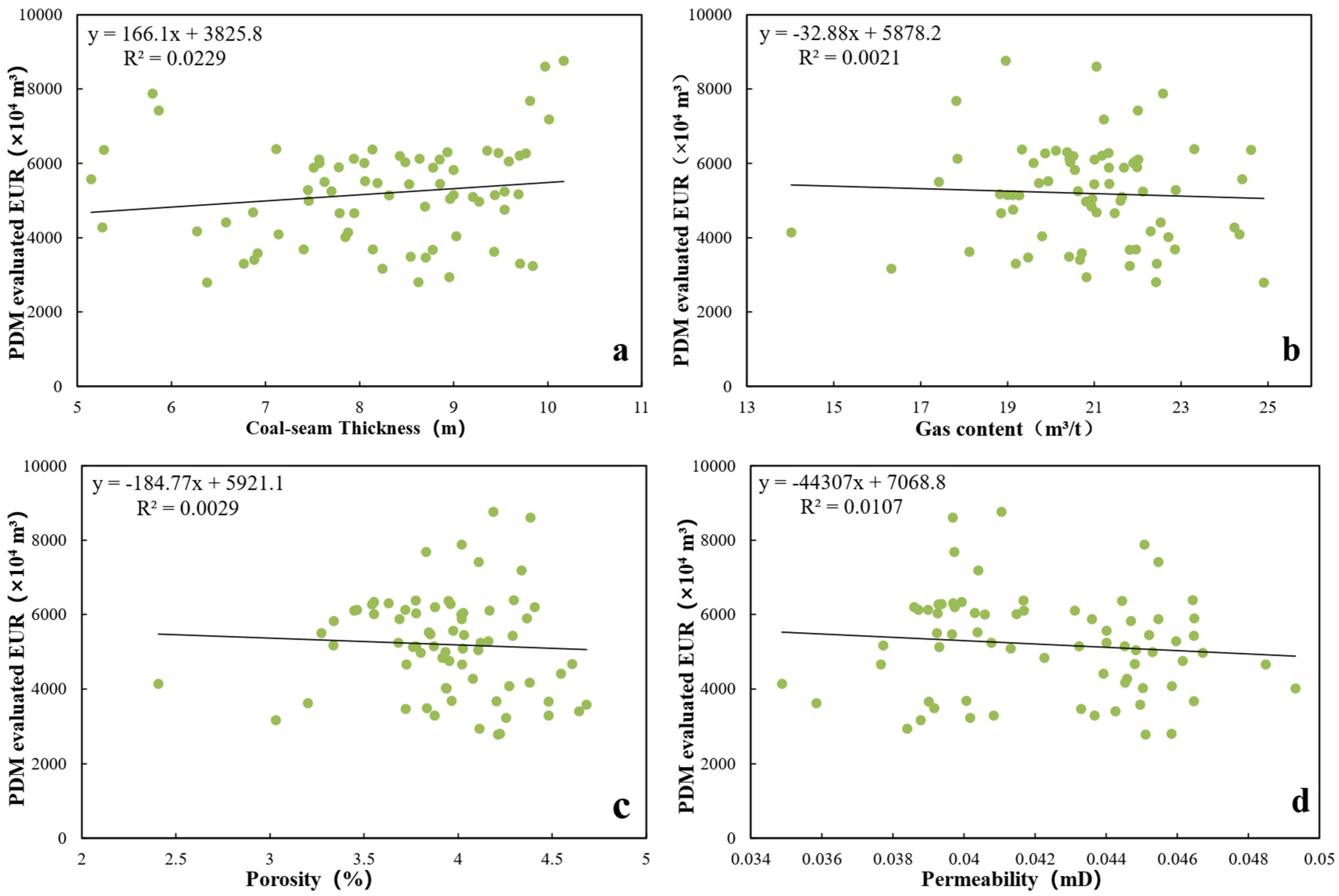
4.1.1. Influence of Geological Conditions

This paper mainly focuses on coal-seam thickness, gas content, porosity, and permeability to discuss the influence of geological conditions on EUR. The survey region has a poor heterogeneity of reservoir physical properties and small variations in porosity (2.4~4.68%) and permeability (0.034~0.049 mD) but large variations in coal-seam thickness (5.1~10.2 m) and gas content (14.0~24.9 m3/t). As shown in the scatter plots of geological conditions and EUR (Figure 3), geological conditions do not have a significant influence on EUR. This finding is inconsistent with the theoretical analysis results. The inconsistency may have two reasons. The influence of geological conditions on EUR is complex and non-linear, and the relationships between geological parameters are intricate, so there is no obvious correlation between geological conditions and EUR. Moreover, as the reservoir resources are highly abundant, the resource abundance under different geological conditions can meet the development needs; that is to say, geological conditions will not restrict EUR.

4.1.2. Influence of Engineering Parameters

This paper focuses on the horizontal length, the number of clusters, the volume of fracturing fluid, and the amount of proppant to analyze the influence of engineering parameters on EUR. According to the scatter plots (Figure 4), the horizontal length, clusters, fracturing fluid, and proppant are, to some extent, positively correlated with EUR. The trend line slope of the scatter plot indicates that the correlation is not significant.
In theory, EUR is determined by geological conditions and engineering parameters. However, in the survey region, both geological conditions and engineering parameters show complicated relationships with EUR. It indicates that geological conditions and engineering parameters have a complex impact on EUR, showing a nonlinear mapping relationship rather than a linear relationship with EUR. Therefore, it is essential to build a nonlinear model to evaluate EUR based on geological conditions and engineering parameters.

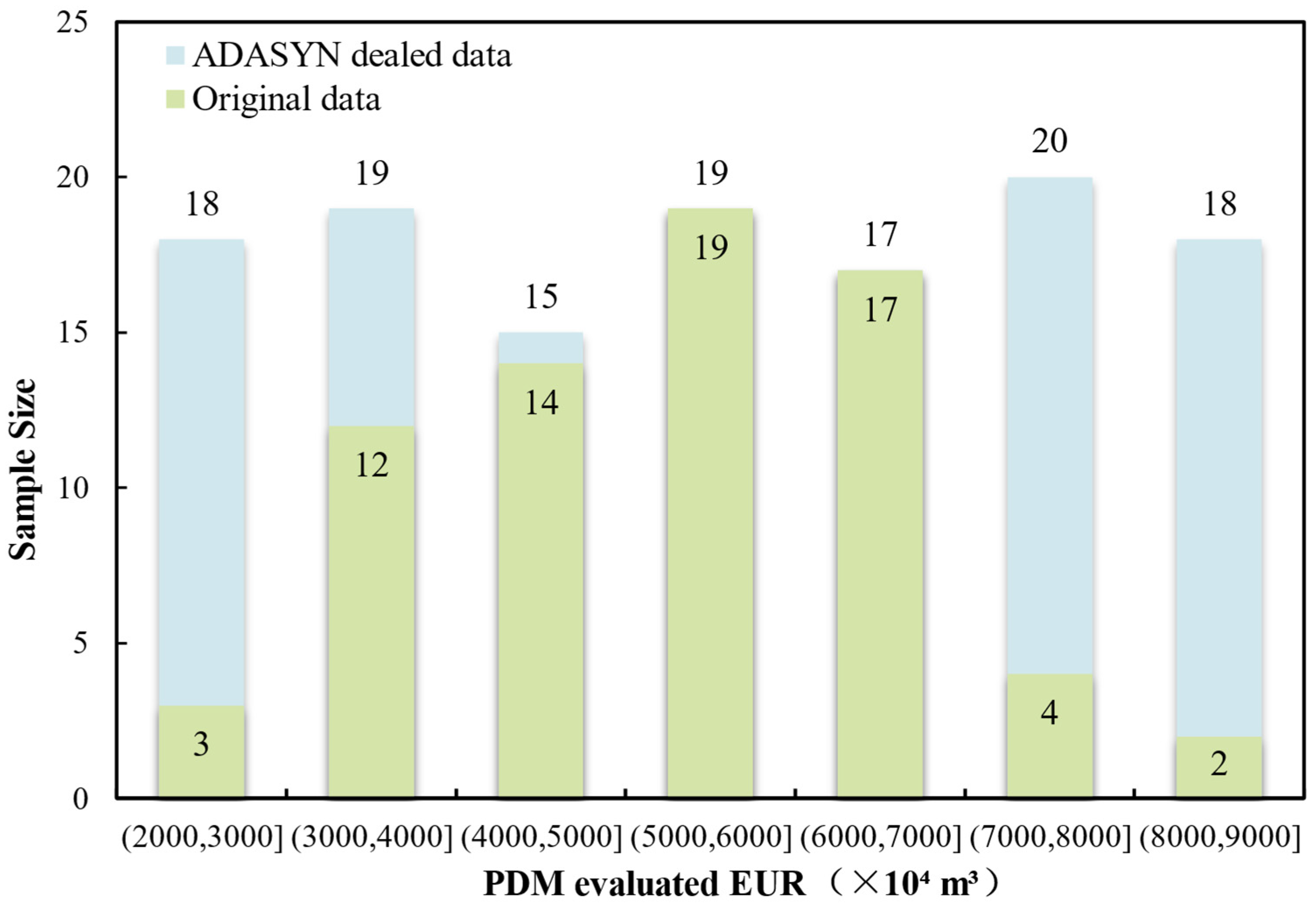
4.2. Data Imbalance Processing

This paper adopts the production decline method to acquire the EUR results of 71 wells and the corresponding geological conditions and engineering parameters and uses them as training data samples for machine learning. EUR falls in the distribution range of 27.89~87.63 million cubic meters. Most EUR values fall in the range of 30~70 million cubic meters. However, few fall in the small-value zone (20–30 million cubic meters) and high-value zone (70–80 million cubic meters), with just three and six samples, respectively (Figure 5). Consequently, it is difficult to capture the data features of the low-value and high-value zones in the model training process and thus reduces the accuracy of model training.
The ADASYN algorithm is used to over-sample the original data to synthesize 55 data samples, increasing the total number of samples to 126. The synthesized data mainly fell in the low-value zone (2000–4000) and the high-value zone (7000–9000) of EUR. After oversampling, the sample distribution in each zone is basically balanced (Figure 5), so oversampling effectively solves the unbalanced distribution of the original data samples.
For example, the support vector machine (SVM) model is trained using the original data (OD) and ADASYN-delt data (ADD). ADD consists of two parts: original data (OD-ADD) and ADASYN-produced data (APD).
To evaluate the effect of the model, we draw the cross plots (Figure 6) of PDM-evaluated EUR and SVR-predicted EUR to compare the model effects of the training set and the test set. The more concentrated the distribution of data points and the closer the trend line slope is to 1, the smaller the model error and the higher the model accuracy. For example, errors of OD in both the high-value and low-value zones of EUR are big. The distribution of EUR OD-ADD is more concentrated, which is particularly obvious in the high-value and low-value zones, and the trend line slope is closer to 1. This indicates that ADASYN oversampling can effectively improve the effect of the machine learning model in solving unbalanced data distribution.
The Mean Absolute Percentage Error (MAPE) of OD and OD-ADD in model training are calculated to compare the model accuracy (Figure 7) to further analyze the improvement of the model effect. The MAPE of OD-ADD is significantly lower than that of OD, indicating that ADASYN oversampling can greatly enhance the accuracy of machine learning model training.

4.3. Machine Learning-Based EUR Evaluation and Model Optimization

4.3.1. Rules of Data Set Division

The random sampling method is used to divide 126 groups of ADASYN-delt data into several data sets to construct the training set, verification set, and test set samples. To ensure the balanced EUR distribution in each data set, this paper divides 126 sets of sample data into intervals according to the EUR value with an interval of 10 million cubic meters (Figure 4) and further divides the data sets in each interval according to the proportion of training set, verification set, and test set (Table 2).

4.3.2. Machine Learning-Based EUR Evaluation Results

The training set, verification set, and test set samples are used to train and verify the BP neural network model, the support vector machine model, and the Gaussian process regression model, respectively.
This research draws the cross plots (Figure 8) of the PDM-evaluated EUR and BPNN-predicated EUR, SVR-predicted EUR, and GPR-predicted EUR, respectively, for the BPNN model, the SVR model, and the GPR model to compare the model effects. According to the comparison results of the three models, the data distribution is concentrated and the trend line slope is close to 1. However, the data distribution of the training set in the GRP model is concentrated on the trend line while the data distribution of its test set is decentralized, indicating a high accuracy of the BPNN model and the SVM model. However, the Gaussian process regression model may bear the risk of overfitting.
The goodness of Fit (R2) and Mean Absolute Percentage Error (MAPE) are statistically analyzed (Table 3) to compare the model effects. The MAPE of the GPR training set is 0.02 and the corresponding figure of its test set is 4.09. The MAPE of the test set is 204.5 times that of the training set, greatly exceeding the threshold overfitting value of 1.5 times. Thus, the GPR model has overfitting problems. Both the BPNN model and the SVM model have good model results. The R2 and MAPE of the test set show that the SVM model is more stable, so the SVM is favorably selected to predict EUR.

4.3.3. Residual Analysis of EUR Evaluation Results Based on Machine Learning

To further assess the accuracy and stability of the machine learning model predictions, this section introduces standard residual analysis. By plotting the standard residuals, we explore the distribution characteristics of the model prediction errors to verify whether there is any systematic bias in the model’s performance.
Standard residuals are used to measure the extent to which predicted values deviate from actual values. When the standard residuals are concentrated within the range of [−3, 3], it indicates that the model’s prediction errors are small and well-distributed, with few outliers and no significant systematic biases.
A comprehensive analysis of the standard residuals for the BPNN, SVR, and GPR models (Figure 9) reveals the following:
(1)
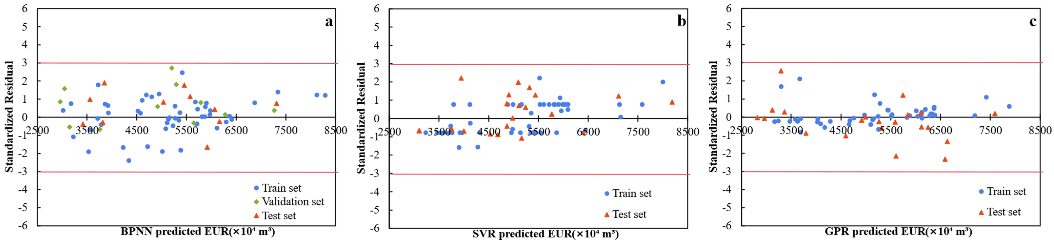
The standard residuals for all three models (BPNN, SVR, and GPR) are distributed within the range of [−3, 3], suggesting that the prediction errors for all three models are generally controllable. In the mid-value range (4500–6500), all models perform well, with residuals concentrated near zero. In the low-value (<4000) and high-value (>7000) ranges, the residuals for all models show greater fluctuation, indicating that the sparsity of boundary samples contributes to the increased errors.
(2)
The BPNN model performs better in the mid-value range but shows slightly weaker generalization ability compared to SVR, with a significant increase in residual fluctuations for boundary samples. This reflects the model’s limited ability to adapt to data from the low and high-value regions. The SVR model demonstrates the best fitting and generalization capabilities, with a higher consistency in the residual distribution between the training and test sets. The prediction errors for both the low and high-value regions are relatively small, and the model exhibits stable performance with strong robustness. The GPR model provides the best fitting results for the training set, but due to overfitting, the residual distribution for the test set is significantly more dispersed, with the weakest generalization ability, particularly for the boundary region, where prediction errors are largest.

4.4. Feature Importance Analysis

The permutation feature importance (PFI) algorithm is used to evaluate the contribution of each feature to predicting the performance of the SVM model selected in this research. To be specific, this research performs feature permutations 10,000 times with a feature value disrupted each time and calculates the changes in the model’s MAPE before and after the permutation. The influence of each feature on model performance is quantified by comparing the difference in MAPE before and after the permutations to determine the contributions of different feature parameters to EUR prediction results.
According to the feature importance analysis results (as shown in Figure 10), all four parameters with the greatest influence on the EUR prediction result are engineering parameters, namely, clusters, the horizontal length, fracturing fluid, and proppant. Geological conditions (coal-seam thickness, porosity, gas content, and permeability) show a smaller impact on the EUR prediction results than engineering parameters. This finding is consistent with the qualitative analysis results of the EUR influencing factors; that is to say, engineering parameters have a significantly positive correlation with EUR but geological conditions do not significantly correlate with EUR. In theory, the abundance and quantity of geological resources can determine the success or failure of the development. The abundance and quantity of geological resources are determined by geological conditions; therefore, the geological conditions should have a significant influence on EUR. However, geological conditions do not significantly influence the EUR of deep coalbed methane in the Daning–Jixian block. Deep coalbed methane in the Daning–Jixian block shows high productivity. This research deduces that the geological resources of the 71 wells involved in this research have a great abundance and quantity to meet the development demand, so the productivity mainly depends on the volume of reservoir reconstruction; that is, engineering parameters.
Engineering parameters not only affect coalbed methane production but are also closely related to development costs. Increasing the number of clusters can enhance the density of the fracture network and gas release, thereby improving production; however, this also requires more complex fracturing operations, which will increase development costs. Longer horizontal sections can cover a larger coal-seam area, resulting in higher production, but extended horizontal lengths also increase drilling and construction time, significantly raising costs, especially in deep coalbed methane development. Increasing the fracturing fluid volume helps facilitate fracture formation and gas flow, thereby enhancing production, but more fracturing fluid means additional costs for chemicals and transportation. Proppants help keep fractures open and enhance gas release, thus improving production, but the procurement and transportation costs of proppants also rise with increased usage. Therefore, when optimizing development plans, it is essential to balance production enhancement with cost control.

5. Conclusions

Taking deep coalbed methane in the Daning–Jixian block of the Ordos Basin, this paper adopts the production decline method to evaluate EUR, processes data with ADASYN, predicts EUR using BPNN, SVM, and GPR models, selects the optimal model, uses the optimal model to analyze feature importance, and gets the following results:
(1)
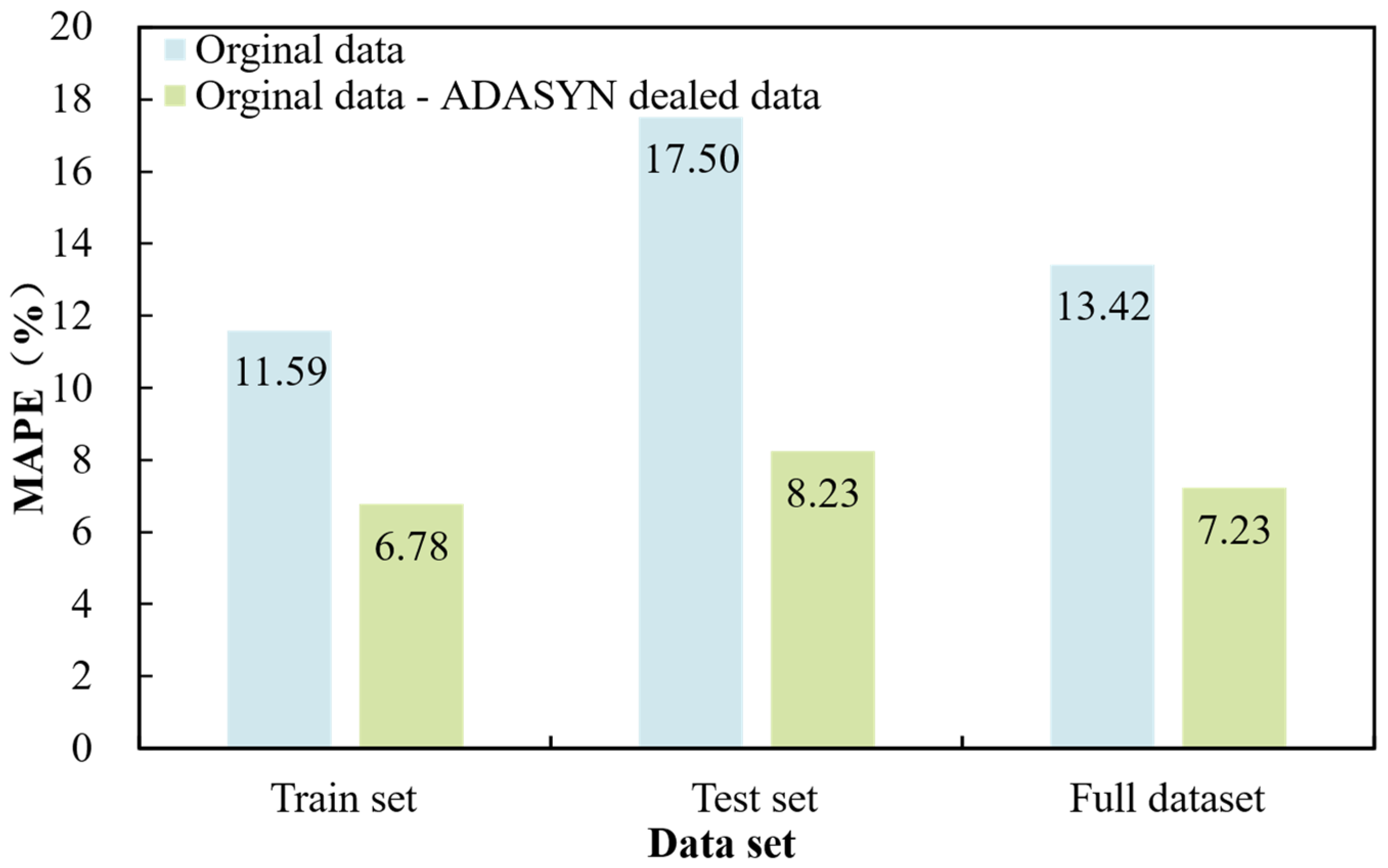
ADASYN oversampling can solve the problem of unbalanced data distribution well, thus remarkably enhancing the model accuracy of machine learning. ADASYN oversampling reduces the training set error of the SVM model from 11.59% to 6.78% and its test set error from 13.42% to 7.23%;
(2)
According to R2 and MAPE results, the GPR model has overfitting problems. The overall performance of the SVM model is better than that of the BPNN model, so the SVM is selected in this research to predict the EUR of deep coalbed methane in the Daning–Jixian block.
(3)
The abundance and amount of geological resources for deep coalbed methane in the Danning–Jixian block can satisfy the development demand and will not impose any restrictions on EUR. EUR is mainly determined by the scale of reservoir reconstruction. Engineering parameters (including clusters, the horizontal length, fracturing fluid, and proppant) are the most important factors influencing the EUR prediction results, while geological conditions (coal-seam thickness, porosity, gas content, and permeability) are the second most important.
Although this study has made certain progress in identifying the key influencing factors of EUR in deep coalbed methane and its prediction methodology, the findings are still subject to constraints in terms of data scale, regional applicability, and methodological limitations. After a thorough analysis, the limitations of this study are summarized as follows:
(1)
The data set used in this study consists of only 71 wells. Although the ADASYN algorithm was applied to address data imbalance and expand the sample size, the overall sample quantity remains limited. This restricts the generalization ability of the model and may affect its applicability under different geological conditions or combinations of engineering parameters.
(2)
This study focuses on a single block in the Ordos Basin (the Daning–Jixian block). As a result, the findings may only be applicable to regions with similar geological conditions. For other areas with distinct geological characteristics or coalbed methane development scenarios, specific evaluation models tailored to their geological and engineering conditions may be required. Nonetheless, this study provides a useful reference for evaluating deep coalbed methane resources in other regions.
(3)
The GPR model exhibited overfitting, which may lead to significant errors when predicting EUR for new wells or undeveloped areas. Such errors could result in deviations in resource evaluation, causing the development potential to be overestimated or underestimated. This may misguide project decision-making and affect the rationality of well placement planning. Moreover, given the high costs associated with deep coalbed methane development, inaccurate predictions caused by overfitting could lead to misestimated project revenues, further increasing economic risks.

Author Contributions

F.W.: Funding acquisition, Methodology; M.W., Writing—original draft, Visualization; Y.W.: Methodology; S.L.: Conceptualization; W.S.: Resources; G.C.: Investigation; Validation, Writing—review and editing; Y.F.: Data curation; X.S.: Visualization; Z.Z.: Validation; Y.L.: Resources. All authors have read and agreed to the published version of the manuscript.

Funding

This study was sponsored by the National Natural Science Foundation of China (No. 42272156) and the Research on Educational Reform of Hainan Higher Education Institutions (No. Hnjg2024-276).

Data Availability Statement

The original contributions presented in this study are included in the article. Further inquiries can be directed to the corresponding author.

Conflicts of Interest

Feng Wang, Mansheng Wu, Yuan Wang, Wei Sun, Yanqing Feng, Xiaosong Shi, ZengPing Zhao, and Ying Liu are employed by the PetroChina Coalbed Methane Company Limited and by the China United Coalbed Methane National Engineering Research Center Co., Ltd. The authors declare that the research was conducted in the absence of any commercial or financial relationships that could be construed as a potential conflict of interest.

References

  1. Luo, P.Y.; Zhu, S.Y. Theoretical and Technical Fundamentals of a 100-Billion-Cubic-Meter-Scale Large Industry of Coalbed Methane in China. Acta Pet. Sin. 2023, 44, 1755–1763. [Google Scholar]
  2. Zhang, D.Y.; Zhu, J.; Zhao, X.L.; Gao, X.; Geng, M.; Chen, G.; Jiao, J.; Liu, S.T. Dynamic assessment of coalbed methane resources and availability in China. J. China Coal Soc. 2018, 43, 1598–1604. [Google Scholar]
  3. Liu, D.M.; Jia, Q.F.; Cai, Y.D. Research progress on coalbed methane reservoir geology and characterization technology in China. Coal Sci. Technol. 2022, 50, 196–203. [Google Scholar]
  4. Xu, F.Y.; Xiao, Z.H.; Chen, D.; Yan, X.; Wu, N.; Li, X.F.; Miao, Y.N. Current status and development direction of coalbed methane exploration technology in China. Coal Sci. Technol. 2019, 47, 205–215. [Google Scholar]
  5. Xu, F.Y.; Yan, X.; Lin, Z.P.; Li, S.G.; Xiong, X.Y.; Yan, D.T.; Wang, H.Y.; Zhang, S.Y.; Xu, B.R.; Ma, X.Y. Research progress and development direction of key technologies for efficient coalbed methane development in China. Coal Geol. Explor. 2022, 50, 1–14. [Google Scholar]
  6. Xu, F.Y.; Wang, C.W.; Xiong, X.Y.; Xu, B.R.; Wang, H.N.; Zhao, X.; Jiang, S.; Song, W.; Wang, Y.B.; Chen, G.J. Evolution law of deep coalbed methane reservoir formation and exploration and development practice in the eastern margin of Ordos Basin. Acta Pet. Sin. 2023, 44, 1764–1780. [Google Scholar]
  7. Xiong, X.Y.; Yan, X.; Xu, F.Y.; Li, S.G.; Nie, Z.H.; Feng, Y.Q.; Liu, Y.; Chen, M.; Sun, J.Y.; Zhou, K. Analysis of multi-factor coupling control mechanism, desorption law and development effect of deep coalbed methane. Acta Pet. Sin. 2023, 44, 1812–1826,1853. [Google Scholar]
  8. An, Q.; Yang, F.; Yang, R.Y.; Huang, Z.W.; Li, G.S.; Gong, Y.J.; Yu, W. Practice and understanding of deep coalbed methane massive hydraulic fracturing in Shenfu Block, Ordos Basin. J. China Coal Soc. 2024, 49, 2376–2393. [Google Scholar]
  9. Ming, Y.; Sun, H.F.; Tang, D.Z.; Xu, L.; Zhang, B.J.; Chen, X.; Xu, C.; Wang, J.X.; Chen, S.D. Potential for the production of deep to ultradeep coalbed methane resources in the Upper Permian Longtan Formation, Sichuan Basin. Coal Geol. Explor. 2024, 52, 102–112. [Google Scholar]
  10. Guo, X.J.; Zhi, D.M.; Mao, X.J.; Wang, X.J.; Yi, S.W.; Zhu, M.; Gan, R.Z.; Wu, X.Q. Discovery and significance of coal measure gas in Junggar Basin. China Pet. Explor. 2021, 26, 38–49. [Google Scholar]
  11. Fan, L.Y.; Zhou, G.X.; Yang, Z.B.; Wang, H.C.; Lu, B.J.; Zhang, B.X.; Chen, Y.H.; Li, C.L.; Wang, Y.Q.; Gu, J.Y. Geological control on differential enrichment of deep coalbed methane in Ordos Basin. Coal Sci. Technol. 2024, 1–13. [Google Scholar]
  12. Xu, F.Y.; Hou, W.; Xiong, X.Y.; Xu, B.R.; Wu, P.; Wang, H.Y.; Feng, K.; Yun, J.; Li, S.G.; Zhang, L. The status and development strategy of coalbed methane industry in China. Pet. Explor. Dev. 2023, 50, 765–783. [Google Scholar] [CrossRef]
  13. Zhao, Y.L.; He, G.; Liu, X.Y.; Zhang, L.H.; Wu, J.F.; Chang, C. A new method for fitting empirical production decline model based on data weighting: A case study on Changning Block of the Sichuan Basin. Nat. Gas Ind. 2022, 42, 66–76. [Google Scholar]
  14. Jiang, R.Z.; He, J.X.; Jiang, Y.; Fan, H.J. Establishment and application of Blasingame production decline analysis method for fractured horizontal well in shale gas reservoirs. Acta Pet. Sin. 2019, 40, 1503–1510. [Google Scholar]
  15. Liu, X.H.; Zou, C.M.; Jiang, Y.D.; Yang, X.F. Basic principles and applications of modern production decline analysis. Nat. Gas Ind. 2010, 5, 50–54. [Google Scholar]
  16. Arps, J.J. Analysis of decline curves. Trans. AIME 1945, 160, 228–247. [Google Scholar] [CrossRef]
  17. Li, K.; Horne, R.N. An analytical model for production decline-curve analysis in naturally fractured reservoirs. SPE Reserv. Eval. Eng. 2005, 8, 197–204. [Google Scholar] [CrossRef]
  18. Ilk, D.; Rushing, J.A.; Perego, A.D.; Blasingame, T.A. Exponential vs. Hyperbolic Decline in Tight Gas Sands—Understanding the Origin and Implications for Reserve Estimates Using Arps’ Decline Curves. In Proceedings of the SPE Annual Technical Conference and Exhibition, Denver, CO, USA, 21–24 September 2008; SPE: Denver, co, USA, 2008; p. SPE-116731-MS. [Google Scholar]
  19. Kupchenko, C.L.; Gault, B.W.; Mattar, L. Tight gas production performance using decline curves. In Proceedings of the SPE Unconventional Resources Conference/Gas Technology Symposium, Calgary, AB, Canada, 16–19 June 2008; SPE: Calgary, AB, Canada, 2008; p. SPE-114991-MS. [Google Scholar]
  20. Song, H.-j.; Su, Y.-h.; Xiong, X.-l.; Liu, Y.; Zhong, S.-c.; Wang, J.-j. EUR evaluation workflow and influence factors for shale gas well. Nat. Gas Geosci. 2019, 30, 1531–1538. [Google Scholar]
  21. Valkó, P.P. Assigning value to stimulation in the Barnett Shale: A simultaneous analysis of 7000 plus production hystories and well completion records. In Proceedings of the SPE Hydraulic Fracturing Technology Conference and Exhibition, The Woodlands, TX, USA, 19–21 January 2009; SPE: The Woodlands, TX, USA, 2009; p. SPE-119369-MS. [Google Scholar]
  22. Gu, Y.F.; Zhang, D.Y.; Bao, Z.D. Permeability prediction using PSO-XGBoost based on logging data. Oil Geophys. Prospect. 2021, 56, 26–37. [Google Scholar]
  23. Li, N.; Xu, B.; Wu, H.; Feng, Z.; Li, Y.; Wang, K.; Liu, P. Application status and prospects of artificial intelligence in well logging and formation evaluation. Acta Pet. Sin. 2021, 42, 508–522. [Google Scholar]
  24. Li, Y.F.; Cheng, J.Y.; Wang, C. Seismic attribute optimization based on support vector machine and coalbed methane prediction. Coal Geol. Explor. 2012, 40, 75–78. [Google Scholar]
  25. Feng, K.; Li, F.; Zhang, S.Y.; Zhao, Y.H.; Zhen, H.B.; Liu, J.J.; Zhu, J. Evaluation and optimization of coalbed methane well production based on production data. Min. Res. Dev. 2023, 43, 52–58. [Google Scholar]
  26. Zhu, Q.Z.; Li, Z.J.; Li, Z.Y.; Wang, S.S.; Sun, R.X.; Wang, Y.T.; Xiao, Y.H.; Wang, J.; Wang, J.Y.; Guan, X.Q. Practice and cognition of efficient CBM development under complex geological conditions: A case study of Zhengzhuang Block, Qinshui Basin. Coal Geol. Explor. 2023, 51, 131–138. [Google Scholar]
  27. Song, H.Q.; Du, S.Y.; Yang, J.S.; Wang, M.Z.; Zhao, Y.; Zhang, J.D.; Zhu, J.W. Forecasting and influencing factor analysis of coalbed methane productivity utilizing intelligent algorithms. Chin. J. Eng. 2024, 46, 614–626. [Google Scholar]
  28. Chawla, N.V.; Bowyer, K.W.; Hall, L.O.; Kegelmeyer, W.P. SMOTE: Synthetic minority over-sampling technique. J. Artif. Intell. Res. 2002, 16, 321–357. [Google Scholar] [CrossRef]
  29. He, H.; Garcia, E.A. Learning from imbalanced data. IEEE Trans. Knowl. Data Eng. 2009, 21, 1263–1284. [Google Scholar]
  30. Tang, S.L.; Tang, D.Z.; Yang, J.S.; Deng, Z.; Li, S.; Chen, S.D.; Feng, P.; Huang, C.; Li, Z.W. Pore structure characteristics and gas storage potential of deep coal reservoirs in Daning-Jixian block of Ordos Basin. Acta Pet. Sin. 2023, 44, 1854–1866,1902. [Google Scholar]
  31. Sun, H.M.; Liu, Z.D.; Xing, X.J.; Liu, Q.; Deng, L.; Zhang, Z.C.; Yang, H.T.; Zhang, L.Z. Fractal characteristics and classification evaluation of pore structure of tight gas reservoirs in Shanxi section of Daning-Jixian area. J. Xi’an Univ. Arts Sci. 2024, 27, 60–67. [Google Scholar]
  32. Li, Y.E.; Chen, G.H.; Cai, Z.X.; Lu, S.F.; Wang, F.; Zhang, Y.J.; Bai, G.S.; Ge, J. Occurrence of methane in organic pores with surrounding free water: A molecular simulation study. Chem. Eng. J. 2024, 497, 155597. [Google Scholar] [CrossRef]
  33. Robertson, S. Generalized hyperbolic equation. In Proceedings of the Paper SPE 18731 Presented at Society of Petroleum Engineers, Richardson, TX, USA, 1 January 1988. [Google Scholar]
  34. Duong, A.N. An unconventional rate decline approach for tight and fracture-dominated gas wells. In Proceedings of the SPE Canada Unconventional Resources Conference, Calgary, AB, Canada, 19–21 October 2010; SPE: Calgary, AB, Canada, 2010; p. SPE-137748-MS. [Google Scholar]
  35. Wang, K.; Li, H.; Wang, J.; Jiang, B.; Bu, C.; Zhang, Q.; Luo, W. Predicting production and estimated ultimate recoveries for shale gas wells: A new methodology approach. Appl. Energy 2017, 206, 1416–1431. [Google Scholar] [CrossRef]
  36. Wang, C.F.; Shao, X.J.; Sun, Y.B.; Xu, H.; Liu, Y.J.; Shi, L. Production decline types and their control factors in coalbed methane wells: A case from Jincheng and Hancheng mining areas. Coal Geol. Explor. 2013, 41, 23–28. [Google Scholar]
  37. Zeng, W.T.; Ge, T.Z.; Wang, Q.; Pang, B.; Liu, Y.H.; Zhang, K.; Yu, L.Z. Exploration of integrated technology for deep coalbed methane drainage in full life cycle: A case study of Daning–Jixian Block. Coal Geol. Explor. 2022, 50, 78–85. [Google Scholar]
  38. Li, M.Z.; Cao, Y.M.; Ding, R.; Deng, Z.; Jiang, K.; Li, Y.Z.; Yao, X.L.; Hou, S.; Hui, H.; Sun, X.G. Gas occurrence and production characteristics of deep coal measure gas and reserve estimation method and indicators in Daning-Jixian block. China Pet. Explor. 2024, 29, 146–159. [Google Scholar]
  39. Min, C.; Wen, G.Q.; Li, X.G.; Zhao, D.Z.; Li, K.C. Research progress and application prospect of interpretable machine learning in artificial intelligence in oil and gas industry. Nat. Gas Ind. 2024, 44, 114–126. [Google Scholar]
  40. Taylor, C.; Vasco, D. Inversion of gravity gradiometry data using a neural network. In SEG Technical Program Expanded Abstracts 1990; Society of Exploration Geophysicists: Houston, TX, USA, 1990; pp. 591–593. [Google Scholar]
  41. Qiao, J.W.; Wang, C.J.; Zhao, H.C.; Shi, Q.M.; Zhang, Y.; Fan, Q.; Wang, D.; Yuan, D.D. A method for predicting the tar yield of tar-rich coals based on the BP neural network using multiple indicators of coal petrography and coal quality. Coal Geol. Explor. 2024, 52, 1–11. [Google Scholar]
  42. Vapnik, V.N. An overview of statistical learning theory. IEEE Trans. Neural Netw. 1999, 10, 988–999. [Google Scholar] [CrossRef] [PubMed]
  43. Schölkopf, B. Learning with Kernels: Support Vector Machines, Regularization, Optimization, and Beyond; MIT Press: Cambridge, MA, USA, 2002. [Google Scholar]
  44. Seeger, M. Gaussian processes for machine learning. Int. J. Neural Syst. 2004, 14, 69–106. [Google Scholar] [CrossRef]
  45. Zhang, W.R.; Chen, X.G.; Qi, J.T.; Zhou, J.B.; Li, N.; Wang, S. Deep Learning and Gaussian Process Regression Based Path Extraction for Visual Navigation under Canopy. Trans. Chin. Soc. Agric. Mach. 2024, 55, 15–26. [Google Scholar]
  46. Lin, Z.Y.; Hao, Z.F.; Yang, X.W. Current state of research on imbalanced datasets classification learning. Appl. Res. Comput. 2008, 25, 332–336. [Google Scholar]
  47. Ye, Z.F.; Wen, Y.M.; Lv, B.L. A survey of imbalanced pattern classification problems. CAAI Trans. Intell. Syst. 2009, 4, 148–156. [Google Scholar]
  48. Lou, X.J.; Sun, Y.X.; Liu, H.T. Cluster boundary oversampling for imbalanced data classification. J. Zhejiang Univ. Eng. 2013, 47, 944–950. [Google Scholar] [CrossRef]
  49. Breiman, L. Random forests. Mach. Learn. 2001, 45, 5–32. [Google Scholar] [CrossRef]
  50. Breiman, L. Statistical modeling: The two cultures (with comments and a rejoinder by the author). Stat. Sci. 2001, 16, 199–231. [Google Scholar] [CrossRef]
  51. Qiu, Y.; Li, S.; Jin, L.; Zhang, M.M.; Wang, J. Bridge abnormal monitoring data identification method based on statistical feature mixture and random forest importance ranking. J. Transduct. Technol. 2022, 35, 756–762. [Google Scholar]
  52. Breiman, L. Bagging predictors. Mach. Learn. 1996, 24, 123–140. [Google Scholar] [CrossRef]
  53. Xiong, X.L. Quantitative evaluation of controlling factors on EUR of shale gas wells in Weiyuan block. China Pet. Explor. 2019, 24, 532–538. [Google Scholar]
Figure 1. Structural location and stratigraphic characteristics of the Daning–Jixian block.
Processes 13 00031 g001
Figure 2. Research methodology framework.
Processes 13 00031 g002
Figure 3. Scatter plots of the correlations between geological conditions and EUR. (a) Scatter plots of the correlation between coal-seam thickness and EUR. (b) Scatter plots of the correlation between gas content and EUR. (c) Scatter plots of the correlation between porosity and EUR. (d) Scatter plots of the correlation between permeability and EUR.
Processes 13 00031 g003
Figure 4. Scatter plots of the correlations between engineering parameters and EUR. (a) Scatter plot of the correlation between horizontal length and EUR. (b) Scatter plot of the correlation between clusters and EUR. (c) Scatter plot of the correlation between fracturing fluid and EUR. B Scatter plot of the correlation between clusters and EUR. (d) Scatter plot of the correlation between proppant and EUR.
Processes 13 00031 g004
Figure 5. Comparison of EUR distribution before and after ADASYN oversampling.
Processes 13 00031 g005
Figure 6. Comparison of model effects before and after EUR data oversampling. (a): SVR model based on original data (OD). (b): Original data in the SVR model based on ADASYN-delt data (OD-ADD).
Processes 13 00031 g006
Figure 7. MAPE comparison histogram of different data samples in model training.
Processes 13 00031 g007
Figure 8. Scatter plots of the three models. (a) Scatter plot of the BPNN. (b) Scatter plot of the SVM model. (c) Scatter plot of the GPR model.
Processes 13 00031 g008
Figure 9. Standard residual plots of the models. (a) Standard residual plot of the BPNN model. (b) Standard residual plot of the SVR model. (c) Standard residual plot of the GPR model.
Processes 13 00031 g009
Figure 10. Feature importance analysis.
Processes 13 00031 g010
Table 1. Production decline models.
Model NameDecline Model EquationEquation NotesApplicable Scope
Arps [16] q = q i e D i t n = 0 q i 1 + D i n t 1 / n 0 < n < 1 q i 1 + D i n t 1 n = 1 q: Monthly gas production calculated by the decline model;
qi: Initial monthly gas production;
Di: Initial decline rate;
n: Decline exponent
Suitable for wells with long production periods and stable bottom-hole flowing pressure
Modified hyperbolic decline [33] q = q i ( 1 + n D i t ) 1 / n ( D > D t ) q i exp ( D t t ) ( D D t ) q: Monthly gas production calculated by the decline model;
qi: Initial monthly gas production;
Di: Initial decline rate;
n: Decline exponent;
Dt: Constrained decline rate
Suitable for wells where the decline rate changes significantly over time
PLE [18] q = q i exp ( D t D 1 n t n ) D = D + D 1 t ( 1 n ) D: Decline rate;
D: Decline rate as production time approaches infinity;
D1 and n: Fitting constants;
Applicable to the unstable flow phase, transitional flow phase, and boundary-dominated flow phase of gas wells
SEPD [21] q = q i exp [ ( t / τ ) n ] τ and n: Fitting constantsApplicable to the unstable flow phase and transitional flow phase of gas wells
Duong [34] q = q i t m e a 1 m ( t 1 m 1 ) q / G p = a t m Gp: Cumulative gas production;
a and m: Fitting constants
Applicable to the linear flow phase of gas wells
Li [35] q = q i e λ ( ln t ) 2 λ: Fitting constantsApplicable to the linear flow phase of gas wells
Table 2. Division of data sets.
ModelTrain Set Proportion (%)Validation Set Proportion (%)Test Set Proportion (%)
BPNN701515
SVR70/30
GPR70/30
Table 3. Comparison of model parameters.
ModelR2MAPE
Train SetValidation SetTest SetTotal DatasetTrain SetValidation SetTest SetTotal Dataset
BPNN0.910.890.830.906.497.798.647.03
SVR0.92/0.880.906.78/8.237.23
GPR0.99/0.970.990.02/4.091.28
Disclaimer/Publisher’s Note: The statements, opinions and data contained in all publications are solely those of the individual author(s) and contributor(s) and not of MDPI and/or the editor(s). MDPI and/or the editor(s) disclaim responsibility for any injury to people or property resulting from any ideas, methods, instructions or products referred to in the content.

