Abstract
This paper presents a critique of the Honey Badger Algorithm (HBA) with regard to its limited exploitation capabilities, susceptibility to local optima, and inadequate pre-exploration mechanisms. In order to address these issues, we propose the Improved Honey Badger Algorithm (IHBA), which integrates the Elite Tangent Search Algorithm (ETSA) and differential mutation strategies. Our approach employs cubic chaotic mapping in the initialization phase and a random value perturbation strategy in the pre-iterative stage to enhance exploration and prevent premature convergence. In the event that the optimal population value remains unaltered across three iterations, the elite tangent search with differential variation is employed to accelerate convergence and enhance precision. Comparative experiments on partial CEC2017 test functions demonstrate that the IHBA achieves faster convergence, greater accuracy, and improved robustness. Moreover, the IHBA is applied to the fault diagnosis of rolling bearings in electric motors to construct the IHBA-VMD-CNN-BiLSTM fault diagnosis model, which quickly and accurately identifies fault types. Experimental verification confirms that this method enhances the speed and accuracy of rolling bearing fault identification compared to traditional approaches.
1. Introduction
Electric motors are essential components in various industries, converting electrical energy into mechanical energy. Rolling bearings are critical for the smooth operation of many motor components, and their failure is one of the leading causes of motor malfunction. Bearing failures account for over 40% of motor faults [1,2], and if not detected early, can lead to severe consequences, such as prolonged downtime, financial losses, and even risks to human health and safety. Therefore, it is crucial to develop effective fault diagnosis techniques to ensure the reliable operation of electric motors, especially in environments with fluctuating loads and harsh conditions.
Recent advancements in swarm intelligence algorithms have provided promising solutions for fault diagnosis. These algorithms, which mimic the collective behavior of natural organisms, have been successfully applied to various optimization problems, including motor fault diagnosis. Popular algorithms include the Sparrow Search Algorithm (SSA) [3], Whale Optimization Algorithm (WOA) [4], Pelican Optimization Algorithm (POA) [5], Gray Wolf Optimization (GWO) [6], Harris Hawk Algorithm (HHO) [7], etc. These algorithms have demonstrated the capacity for effective global search and adaptability. However, despite their advantages, these algorithms face significant challenges, including premature convergence, limited exploitation capabilities, and susceptibility to local optima, which hinder their performance in complex fault diagnosis tasks.
The Honey Badger Algorithm (HBA), introduced by Fatma et al. in 2021 [8], is inspired by the foraging behavior of honey badgers. While it offers several advantages, such as a simple structure and few adjustable parameters, HBA struggles with issues like inadequate exploration and a slow convergence rate. In response to these shortcomings, numerous modifications have been proposed, such as incorporating reverse learning strategies [9], chaotic mapping [10], and hybrid approaches [11]. However, these improvements often involve increased complexity and do not fully address the underlying limitations in the algorithm’s exploration and exploitation balance.
In this paper, we introduce the Improved Honey Badger Algorithm (IHBA), which integrates the Elite Tangent Search Algorithm (ETSA) and differential mutation strategies to overcome the limitations of traditional HBA. Our proposed method improves exploration by employing cubic chaotic mapping during the initialization phase and utilizes a random value perturbation strategy in the pre-iterative stage to prevent premature convergence. Moreover, when the optimal population value remains unchanged for three consecutive iterations, an elite tangent search with differential variation is triggered to enhance convergence speed and precision. We validate the performance of the IHBA through comparative experiments on several CEC2017 test functions, demonstrating that the IHBA significantly outperforms the traditional HBA in terms of convergence speed, accuracy, and robustness. To further assess the advantages of the IHBA, we conduct ablation experiments comparing it with the original HBA, Dung Beetle Optimizer (DBO) [12], Coati Optimization Algorithm (COA) [13], Osprey Optimization Algorithm (OOA) [14], Beluga Whale Optimization (BWO) [15], Osprey–Cauchy–Sparrow Search Algorithm (OCSSA) [16], and Harris Hawk Algorithm (HHO) [7]. The experimental results clearly show that the IHBA achieves a notable improvement in both the speed of convergence and the accuracy of the optimization process, with enhanced robustness. Furthermore, the IHBA is successfully applied to the fault diagnosis of rolling bearings in electric motors, where we develop an IHBA-VMD-CNN-BiLSTM fault diagnosis model. The experimental results validate that this method significantly improves the speed and accuracy of fault detection, providing a more reliable solution for motor condition monitoring than traditional approaches.
The contributions of this paper are twofold:
- (1)
- The development of the IHBA addresses the key shortcomings of the original HBA by enhancing exploration and accelerating convergence.
- (2)
- The successful application of the IHBA in motor bearing fault diagnosis, providing a novel approach to improving fault detection accuracy in industrial settings.
2. Honey Badger Algorithm (HBA)
The Honey Badger Algorithm (HBA) is a metaheuristic algorithm designed to tackle continuous optimization problems. It mimics the intelligent foraging behavior exhibited by honey badgers in nature and boasts advantages such as high efficiency, a straightforward structure, and ease of implementation [8]. The HBA is structured into two distinct phases as follows, the “Digging Phase” and the “Honey Phase”, which are elaborated upon as follows:
Step 1: Initialization phase. We initialize the number of honey badgers (population size ) and their respective positions based on Equation (1) as follows:
where is the honey badger position referring to a candidate solution in a population of , while and are, respectively, the lower and upper bounds of the search domain, [1, 2, …, ], and is a random number between 0 and 1.
Step 2: Defining intensity (). Intensity is related to concentration strength of the prey and distance between it and the honey badger. is the smell intensity of the prey; if the smell intensity is high, the motion will be fast and vice versa, as defined by Equation (2).
where is a random number between 0 and 1, is the source strength or concentration strength, denotes the distance between prey and the badger, and is the current global optimal food source location, i.e., the optimal solution.
Step 3: Update density factor. The density factor () controls time-varying randomization to ensure the smooth transition from exploration to exploitation. We update the decreasing factor α that decreases with iterations to decrease randomization with time, using Equation (5) as follows:
where is the number of current iterations and is the maximum number of iterations, (default = 2).
Step 4: Digging phase. In the digging phase, a honey badger performs actions in a Cardioid shape. The Cardioid motion can be simulated by Equation (4) as follows:
where is the updated position of the honey badger individual ; , , and are three different random numbers between 0 and 1; and works as the flag that alters search direction, which is determined using Equation (7) as follows:
where is a random number between 0 and 1. In the digging phase, a honey badger heavily relies on the smell intensity, , of the prey, ; the distance between the badger and the prey, ; and the time-varying search influence factor, . Moreover, during the digging phase, a badger may receive disturbances, , allowing it to find an even better prey location.
Step 5: Honey phase. The case of a honey badger following a honey guide bird to reach beehive can be simulated using Equation (8) as follows:
where is a random number between 0 and 1.
3. Improved Honey Badger Algorithm (IHBA)
Like other heuristic algorithms, HBA is premature and susceptible to local optimization in some complex problems. This phenomenon constrains the algorithm’s precision and offers significant potential for enhancement. The improved algorithm introduces several new mechanisms, including a cubic chaotic mapping mechanism, a random value perturbation strategy, an elite tangent search, and a differential mutation strategy.
3.1. Cubic Chaotic Mapping
As the initial population of the basic honey badger search algorithm is randomly generated, it is impossible to guarantee that the initial positions of the individuals are uniformly distributed in the search space. This has an impact on the search speed and optimization performance of the algorithm. The IHBA initialization process incorporates cubic mapping to enhance the traversal of the initial population.
where is cubic chaotic sequence, .
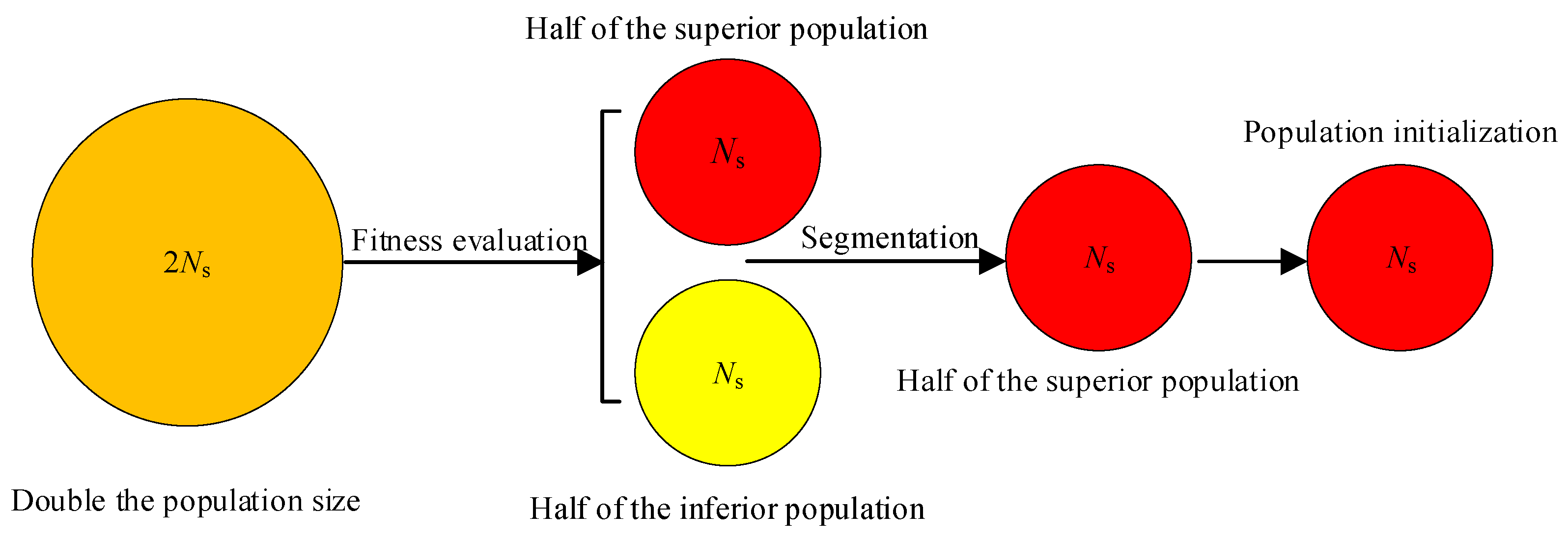
In the initial population generation process utilizing chaotic mapping, solutions with inferior or intermediate positions may be produced. These solutions may prove unfavorable for the subsequent search for the optimal solution or may impede the convergence of the algorithm. Accordingly, a population filtering mechanism is employed in the HBA of elite tangent search with differential variation, whereby solutions with superior initial positions are excluded. As illustrated in Figure 1, the number of solutions is initially generated at twice the expected value during the initialization phase. Subsequently, the optimal half of the solutions is selected as the initial population based on the calculated fitness values.

Figure 1.
Schematic diagram of the population filtering process.
The combination of cubic chaotic mapping with elite tangent search and differential variation enables the HBA to generate populations that are more closely aligned with the optimal solution location during the initialization phase. The pseudocode of the population filtering mechanism using cubic chaotic mapping is illustrated in Algorithm 1.
| Algorithm 1: Population filtering mechanism |
| Initialization of honey badger population size ; 1. Use Equation (9) to generate a population with solutions with random positions; 2. Calculate the fitness function value for each solutions; 3. Sort all individuals according to their fitness function values in descending order; 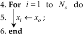 7. Return . |
3.2. Random Value Perturbation Strategy
In the IHBA, a key coefficient, , is introduced to determine the strategy of honey badger position updating, aimed at balancing the algorithm’s global search capability and local convergence speed. The design of this coefficient incorporates the ideas of linear decreasing and stochastic perturbation in order to dynamically adjust the search strategy so as to avoid premature convergence and enhance the algorithm’s global optimization seeking ability. The expression for is as follows:
where , whose value decreases linearly from 2 to 0, and is a random number within (0, 1).
At the beginning of the iteration ( is small), the value of is close to 2, which makes the absolute value of greater than or equal to 1. Especially when is close to 1, the algorithm tends to perform a search strategy with random individual perturbations, which increases the traversal of the search space and helps discover the globally optimal solution. As the number of iterations increases, gradually decreases, resulting in the absolute value of tending to 0. In the later stages of the iteration, the algorithm relies more on the population optimum for position updating, which facilitates the local convergence of the algorithm and accelerates the convergence to the optimal solution.
When , the algorithm performs a search strategy with randomized individual perturbations. This means that the honey badger’s position update does not only depend on the current best individual, , but is also influenced by a random individual, which helps the algorithm go beyond the local optimum and increase the diversity of the search.
Digging phase:
Honey phase:
When , the algorithm returns to the -based position update strategy, which helps the algorithm to perform a fine-grained search in the vicinity of the discovered high-quality solutions, thus speeding up the convergence.
3.3. Elite Tangent Search and Differential Mutation Strategy
The following elite tangent search with a differential variation strategy is performed when the population is iterating and the best value found three times remains unchanged.
Elite subpopulation: In each iteration, the top half of individuals with lower fitness (i.e., better performance, since usually lower fitness values indicate better solutions) are classified into the elite subpopulation based on their fitness value. The elite subpopulation contains the best individuals in the current population, retaining the best solutions. This aims to protect these excellent solutions from being corrupted by subsequent genetic manipulations while allowing them to serve as the basis for future iterations.
Migration strategy for elite subpopulation: When an individual is close to the current optimal solution, it searches the area around it. This behavior, called local search, can improve the convergence speed and solution accuracy. Because the fitness of the elite subpopulation is close to the current optimal solution, the elite subpopulation is allowed to develop locally to improve convergence speed and solution accuracy.
The migration strategy of the elite subpopulation is updated by incorporating the Tangent Search Algorithm (TSA) of Reference [17] used for position updating.
where is the best current solution used to guide the search process towards the best solution, .
Exploration Subpopulation: The second half of the individuals are classified into the exploration subpopulation as opposed to the elite subpopulation. These individuals are usually more highly adapted, i.e., poorer performers. The main purpose of the exploring subpopulation is to explore new regions in the solution space through genetic manipulation to find potentially superior solutions. Since these individuals are not the current best, they are more likely to generate new, possibly superior solutions through operations such as mutation.
Exploration of the evolutionary strategy of the subpopulation: From Equation (13), it can be seen that in the HBA, the position of the honey badger individuals in the population is updated by generating new individuals in the vicinity of the current individual and the current optimal individual , which means that the other individuals in the population move towards . If is a local optimal solution, as the iteration continues, the honey badger individuals in the population gather around , which leads to poor population diversity and makes the algorithm converge prematurely; therefore, to solve these problems, this paper adopts a differential mutation strategy. Inspired by the variation strategy in the differential evolutionary algorithm, a stochastic difference is performed using the current honey badger individual, the current optimal individual, and a randomly selected honey badger individual in the population in order to generate a new individual, which is implemented using Equation (15).
where is the differential evolutionary contraction factor set to 0.4; , , and are randomly selected honey badger individuals. The pseudocode of the IHBA is shown in Algorithm 2.
| Algorithm 2: Pseudocode of the IHBA. |
| Input: |
| Set honey badger population size ; |
| Maximum number of iterations ; |
| Dimension ; |
| Lower bound , upper bound ; |
| Set parameters: constant , attraction factor ; |
| Output: |
| : Global best fitness; |
| : Position of the global best individual; |
| 1. Initialize the population using Algorithm 1; |
| 2. Evaluate the fitness of each honey badger position using objective function and assign to , [1, 2, …, Ns]; |
| 3. Save best position and assign fitness to ; |
| 4. while do |
| 5. Update the decreasing factor using Equation (5); |
| 6. For to do |
| 7. Calculate the intensity using Equation (2); |
| 8. Compute the adaptation parameter using Equation (10); |
| 9. if then |
| 10. if then 11. Update the position using Equation (11), Select a random individual instead of the globally optimal ; 12. else |
| 13. Update the position using Equation (12); 14. end if |
| 15. else |
| 16. if then 17. Update the position using Equation (6); 18. else 19. Update the position using Equation (8); 20. end if |
| 21. end if 22. Evaluate the new individual and assign to the fitness ; 23. if then 24. Set and ; 25. end if 26. if then 27. Set and ; 28. end if 29. if remains unchanged for three consecutive iterations, then execute the elite tangent and differential mutation strategies then 30. Sort the population fitness in ascending order; 31. Divide the population into two groups (optimal half) as elite subgroups and after as exploration subgroups); 32. for to do 33. Generate a random angle θ in the range [0, π/2.1]; 34. Calculate the step size using Equation (14); 35. if == then 36. Update the position using Equation (13(a)); 37. else 38. Update the position using Equation (13(b)); 39. end if 40. end for 41. for to do 42. Randomly select three distinct individuals rand1, rand2, rand3 from the population; 43. Update the position using Equation (15); 44. end for 45. end if 46. if then 47. Set and ; 48. end if 49. if then 50. Set = and ; 51. end if |
| 52. end for |
| 53. end while Stop criteria satisfied. |
| 54. Return , . |
4. Experiment and Results
To assess the optimization performance of the Improved Honey Badger Algorithm (IHBA), we selected 12 benchmark test functions from the CEC2017 suite, each possessing distinct characteristics. For the comparative experiments, we evaluated the IHBA against the following seven other algorithms: the original HBA, COA, DBO, OCSSA, BWO, OOA, and HHO.
To guarantee the fairness of our experimental evaluations, we established a consistent simulation environment using MATLAB R2023a on a Windows 11 operating system powered by an Intel (R) Core (TM) i7-11800H @ 2.3 GHz CPU (The manufacturer of the equipment is Intel Corporation, sourced from Santa Clara, CA, USA.) with 16.0 GB of RAM. Before presenting the results, we outline the experimental setup and crucial parameter settings, detailed in Table 1. The significance of these settings lies in ensuring a level playing field for all algorithms being compared. Specifically, we set the maximum number of iterations to 500 for all algorithms, maintained a population size of 30, and conducted each experiment independently 30 times to ensure statistical reliability.

Table 1.
Main parameter settings.
4.1. Test Function
The 13 test functions selected in this paper are shown in Table 2. and are unimodal functions that have no local minima but only global minima, and these functions test the convergence of the algorithm. , , , and are simple multimodal functions with local extreme points that are used to test the ability of the algorithm to jump out of the local optimum. , , , and are hybrid functions, with each subfunction being assigned a certain weight. and are composition functions composed of at least three hybrid functions or CEC2017 benchmark functions rotated and shifted, and each subfunction has an additional bias value and a weight, which further increase the optimization difficulty of the algorithm, and multiple test functions can fully verify the algorithm’s solution performance.
Table 2.
Test function.
4.2. Results and Discussions
4.2.1. CEC2017 Test Function Set Optimization Experiment
This section presents and discusses the experimental results obtained by evaluating eight algorithms across 13 test functions in 10-dimensional, 30-dimensional, and 50-dimensional spaces. Each experiment was independently replicated 30 times to ensure statistical reliability, and the comprehensive results are summarized in Table 3. We undertake a detailed analysis of the performance of each algorithm, focusing on their mean and variance in achieving optimal solutions. This analysis highlights key consistent observations and patterns across different dimensions and test functions.
Table 3.
Optimization results and comparison for CEC-2017 test functions in three different dimensions.
Table 3 demonstrates that the optimized IHBA outperforms the seven comparison algorithms across most functions and dimensions, showcasing superior optimization capabilities and achieving outstanding results.
In the 10-dimensional case, the IHBA achieves the optimal average value across all tested functions, demonstrating superior optimization performance compared to the other seven comparison algorithms. Specifically, for functions and , the IHBA attains the best optimal values, average values, and standard deviations, indicating its strong consistency and solving ability in both unimodal and simple multimodal problems. For function , the standard deviation of the IHBA is slightly inferior to that of OCSSA; however, the IHBA still outperforms the other six comparison algorithms, showcasing high competitiveness. Regarding function , the IHBA matches the optimal values of the OCSSA, HBA, and HHO and surpasses the other four comparison algorithms. For functions , , , , , and , the IHBA exhibits superior optimal values, average values, and standard deviations compared to the other seven comparison algorithms, indicating strong robustness on multimodal and hybrid functions. In the case of function , the average value of the IHBA is slightly inferior to that of the DBO algorithm but exceeds the other six comparison algorithms, and its standard deviation is slightly lower than BWO, OOA, DBO, and COA but better than the other three comparison algorithms. For function , the standard deviation of the IHBA is slightly inferior to that of the DBO algorithm, but its optimal and average values are superior to the other six comparison algorithms.
In the 30-dimensional case, the IHBA demonstrates superior optimization capabilities, particularly in simple multimodal and hybrid functions, while maintaining strong stability and global exploration. Specifically, for unimodal function , the IHBA achieves superior optimal and average values compared to the other seven comparison algorithms, with its standard deviation being slightly inferior to OCSSA but better than the other six comparison algorithms. For unimodal function , the IHBA outperforms the other seven comparison algorithms in terms of optimal value, standard deviation, and average value. Regarding the simple multimodal function , the IHBA achieves better optimal and average values than the other seven comparison algorithms, although its standard deviation is slightly inferior to the HBA. For the simple multimodal function , the IHBA attains superior optimal and average values compared to the other seven comparison algorithms, with its standard deviation being slightly inferior to the BWO and COA. In the case of simple multimodal functions and , the IHBA achieves superior optimal values, standard deviations, and average values compared to the other seven comparison algorithms. For hybrid functions and , the IHBA demonstrates better optimal values, average values, and standard deviations than the other seven comparison algorithms. Regarding the hybrid function , the IHBA achieves a superior optimal value and standard deviation compared to the other seven comparison algorithms, although its average value is slightly inferior to the OCSSA and better than the other six comparison algorithms. For hybrid function , the IHBA’s optimal and average values surpass those of the other seven comparison algorithms, while its standard deviation is slightly inferior to that of the DBO. In the case of the composition function , the IHBA exhibits a better standard deviation than the other seven comparison algorithms, though its optimal and average values are slightly inferior to the OCSSA. Lastly, for the composition function , the IHBA achieves the best optimal values, average values, and standard deviations.
In the 50-dimensional case, the IHBA continues to demonstrate strong optimization capabilities, particularly in unimodal, hybrid, and composition functions. However, the stability performance of certain simple multimodal functions shows variability. Specifically, for unimodal functions and , the IHBA achieves superior optimal values, standard deviations, and average values compared to the other seven comparison algorithms. Regarding the simple multimodal function , the optimal value of the IHBA is slightly inferior to that of the HBA, yet it surpasses the other six comparison algorithms in terms of optimal value, standard deviation, and average value. For simple multimodal functions , , and , the IHBA attains the best optimal and average values, although its standard deviation is less favorable. In the case of hybrid functions , , and , the IHBA records the highest optimal values, average values, and standard deviations. For the hybrid function , the optimal and average values of the IHBA exceed those of the other seven comparison algorithms, while its standard deviation is marginally inferior to that of the OCSSA. Lastly, for composition functions and , the IHBA achieves the best optimal values, average values, and standard deviations.
The analysis of the optimization results indicates that the IHBA outperforms the other algorithms on the CEC 2017 benchmark, demonstrating superiority across multiple dimensions. It is also exceptionally effective in solving high-dimensional and complex problems, particularly compared to the HBA. Experimental findings show that the enhanced strategy proposed in this paper substantially enhances both the accuracy and stability of the HBA.
Evaluating the complexity of an algorithm by directly comparing its running time is an intuitive method. Table 4 provides a detailed list of the execution times of the IHBA and HBA on 12 test functions. It is evident from the data in the table that the IHBA generally outperforms the HBA in terms of runtime across all test functions. In addition, with the increase in problem dimensions, both the IHBA and HBA show an upward trend in computation time.
Table 4.
Average time for CEC-2017 test functions in three different dimensions.
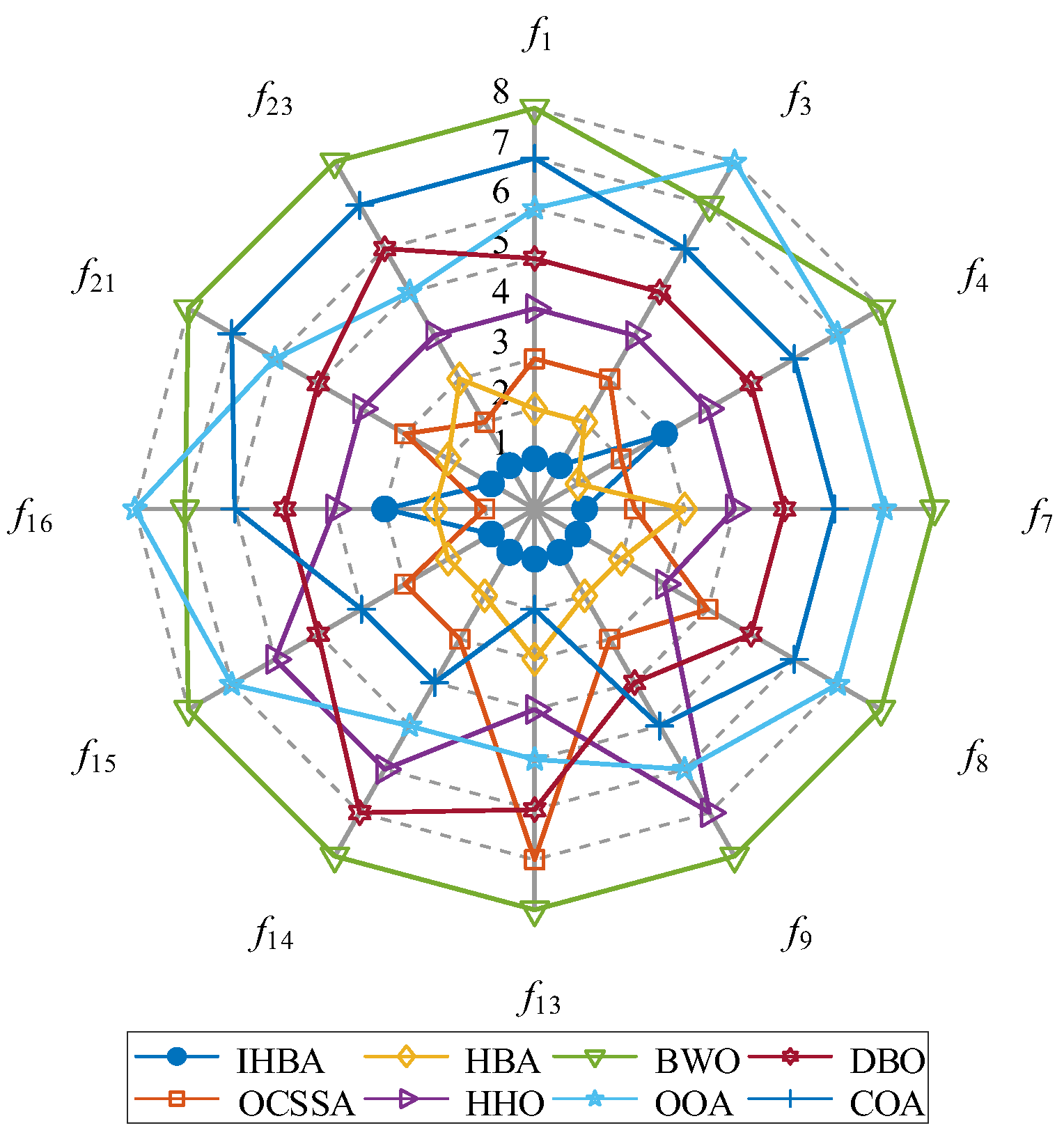
Figure 2 presents a radar chart that analyzes the performance of the IHBA compared to seven other benchmark algorithms using the CEC2017 test functions. The IHBA demonstrates superior performance across multiple dimensions, highlighting its effectiveness in tackling complex optimization problems. Specifically, the IHBA excels in convergence speed, solution accuracy, and algorithm stability, outperforming its counterparts, especially in handling multimodal functions and high-dimensional optimization scenarios. Additionally, the IHBA achieves a balanced trade-off between exploration and exploitation, effectively preventing premature convergence while maintaining robust global search capabilities. In contrast, although some competing algorithms may exhibit strengths in specific test functions, their performance lacks the consistency and comprehensiveness demonstrated by the IHBA. The analysis derived from the radar chart underscores the IHBA’s enhanced adaptability and robustness, positioning it as a highly competitive method within the evolutionary algorithm landscape. These findings suggest that the IHBA is well-suited for diverse optimization challenges, offering reliable and efficient solutions across various complex environments.
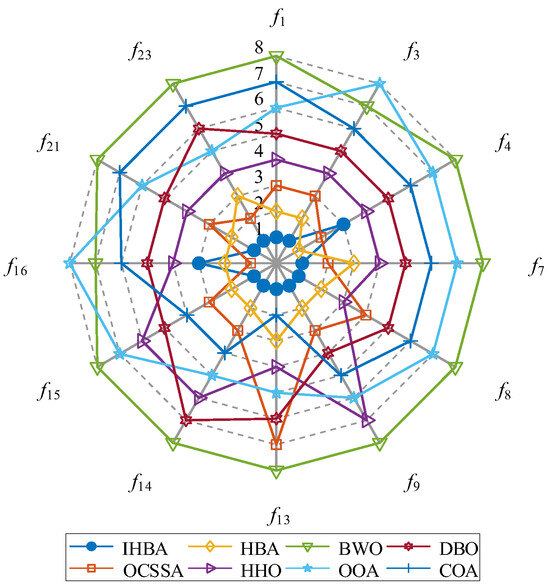
Figure 2.
Radar chart of sort of algorithms.
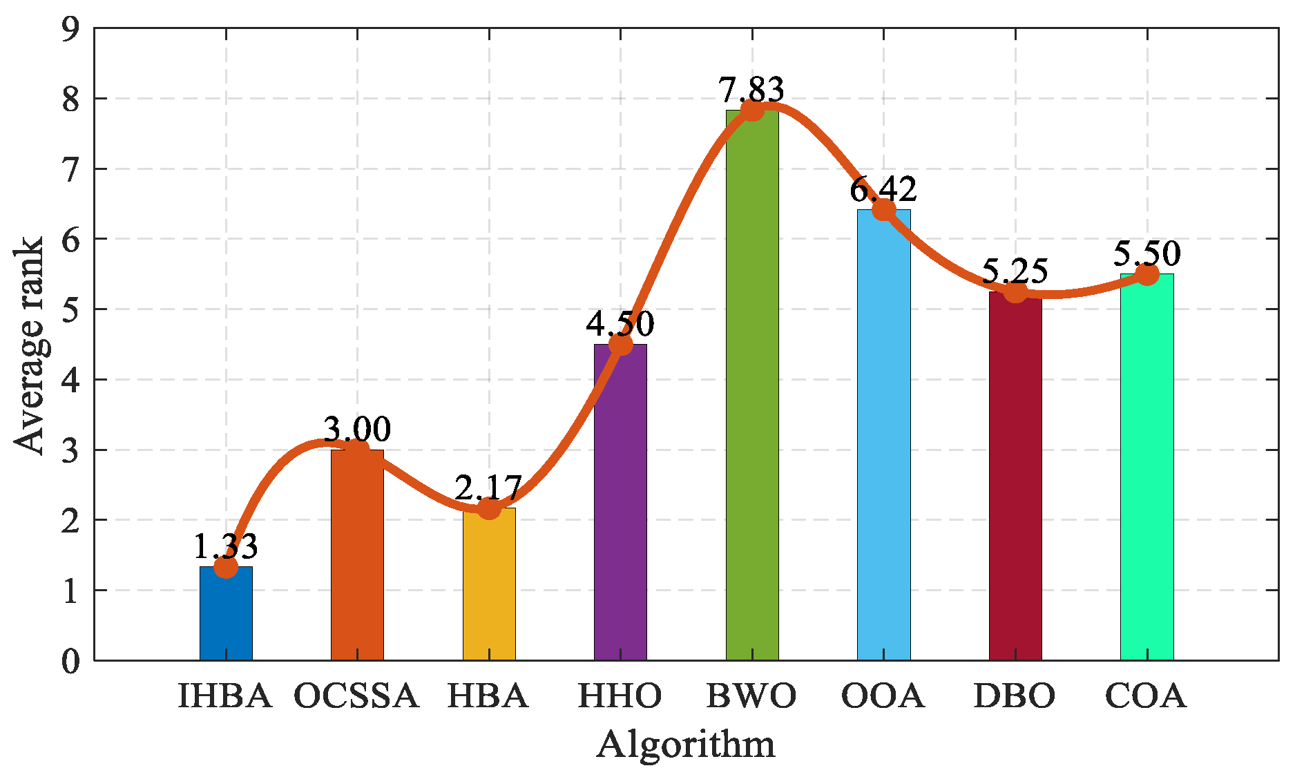
To further compare and analyze the optimization-seeking ability of the improved algorithms, the average fitness results of each algorithm are ranked, and the standard deviations are compared to see if they are equal. The rankings are tied if both the mean and standard deviation are equal. A lower average performance ranking result for the algorithm indicates a superior optimization ability and enhanced optimization search performance. Figure 3 demonstrates the average merit-seeking ranking results of various algorithms. The IHBA is ranked first, with an average ranking result of 1.33, while for the OCSSA, HBA, HHO, BWO, OOA, DBO, and COA, the average ranking results are 3.00, 2.17, 4.50, 7.83, 6.42, 5.25, and 5.50, respectively. From the average ranking results, it can be seen that the ability of the IHBA to find the best results is better than the other seven compared algorithms.

Figure 3.
Results of the sort of average performance.
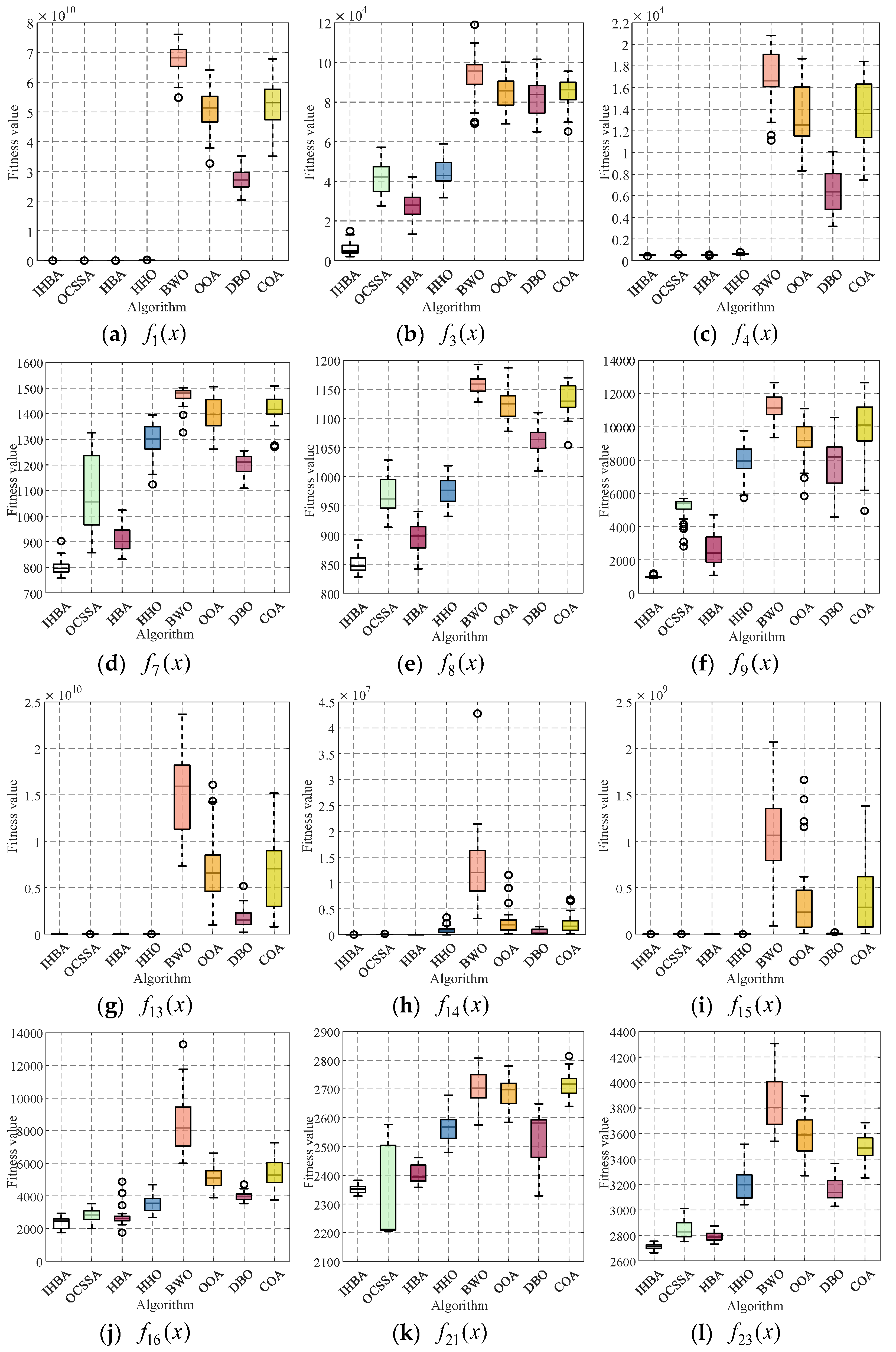
To analyze the distribution characteristics of the IHBA optimization results, box plots were drawn based on the results of each algorithm running independently for 30 times, as shown in Figure 4. The upper and lower boundaries of each box represent the upper and lower quartiles, respectively, and the center line of each box is the median of the 30 optimization results. The symbol “o” indicates the outliers within the box. It can be seen from the box plots that, except for Figure 4e,j, the 30 optimization results of the IHBA are relatively concentrated. Therefore, the improved algorithm in this paper is strong and robust.
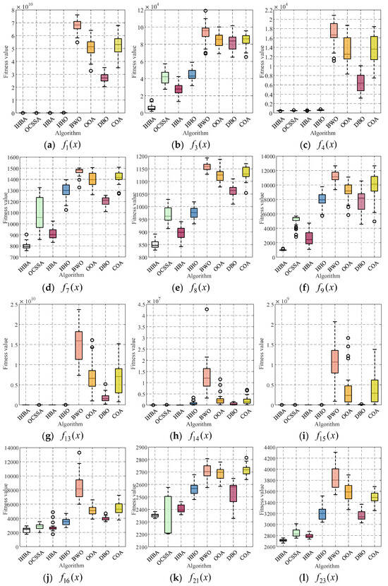
Figure 4.
Convergence boxplot of the test function in 30-dimensional spaces.
Boxplots can reflect the stability of a set of data. The boxplots of the algorithm on 12 representative test functions are plotted in Figure 4, and it is found that the IHBA solves the problem in a more stable manner than the other algorithms, and the distribution of the convergence values is more centralized, which is obviously more superior to the other algorithms and indicates that the IHBA has a better robustness.
4.2.2. Wilcoxon Rank Sum Test
The Wilcoxon rank sum test is a commonly used hypothesis test for analyzing significant algorithm differences. It is widely employed to verify the effectiveness of optimization algorithm improvement strategies and ascertain whether there are significant differences between various algorithms.
The test results are presented in Table 5, where the p-values determine whether a significant difference exists. The significance level is set at the commonly used value of 0.05. If p < 0.5, the null hypothesis can be rejected, indicating a significant difference between the two compared algorithms. Based on the statistical test results, it is evident that the p-values for the IHBA, when compared to the other seven algorithms, are predominantly less than 0.05. This suggests a significant difference in search capability between the improved and comparative algorithms, indicating its statistical superiority.
Table 5.
The p-values of the Wilcoxon rank sum test (dimension 30) in CEC2017.
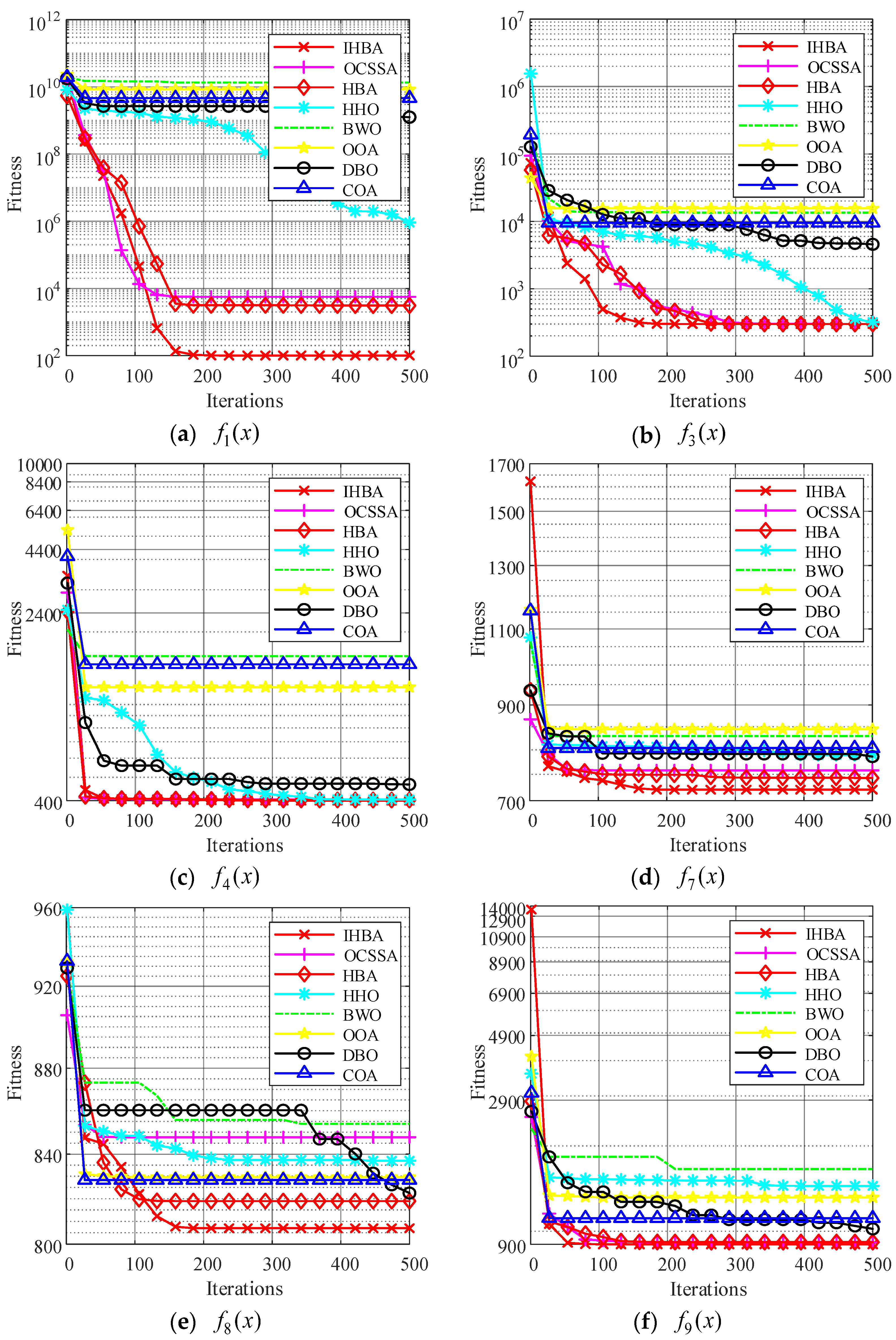
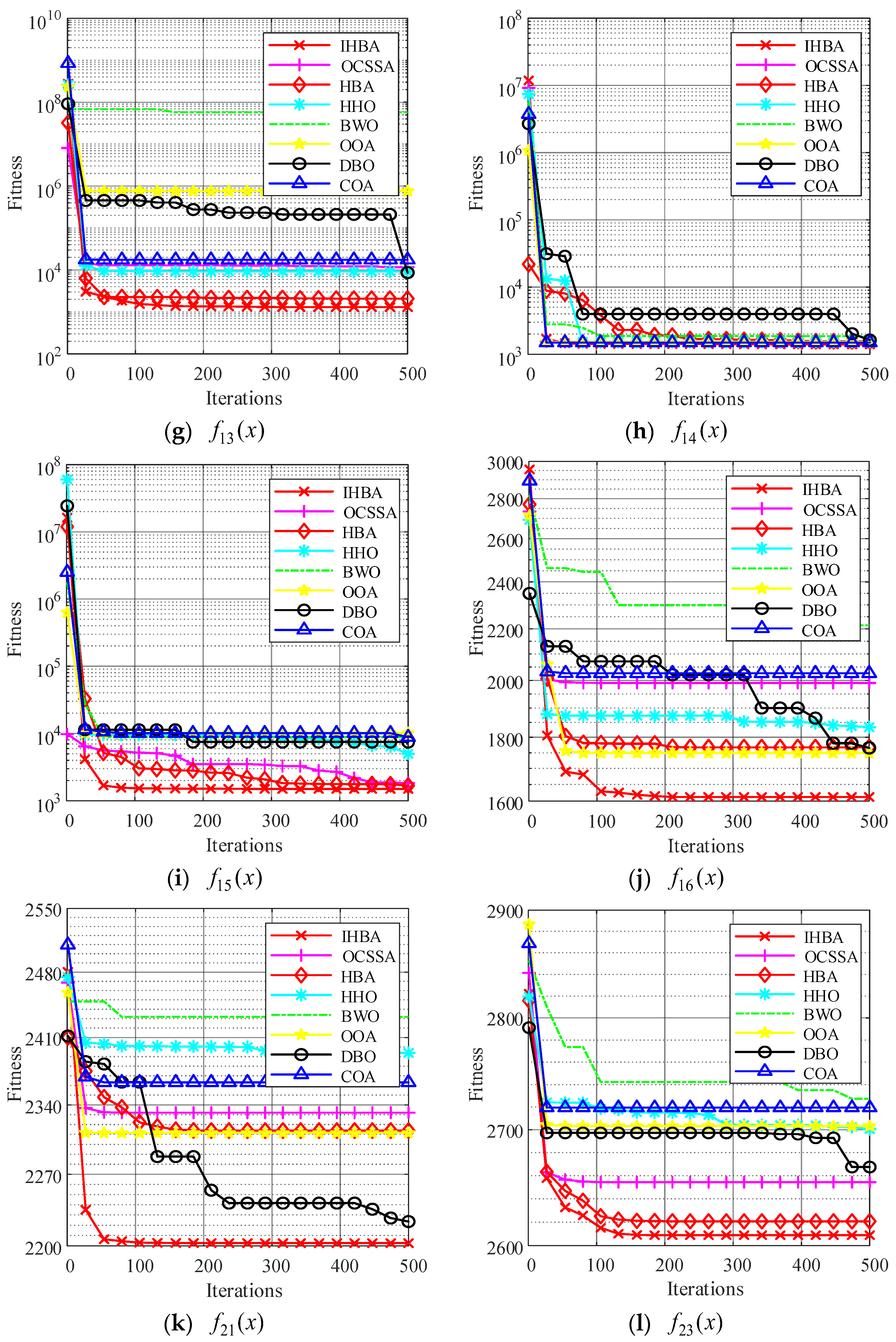
4.2.3. CEC2017 Convergence Curve of the Test Function Set
To verify the convergence performance of the improved algorithm and to visually compare the convergence speeds of different algorithms, we compared the convergence curves of swarm intelligence algorithms when solving function extremum problems.
Observing the aforementioned convergence curve, it can be concluded that the IHBA exhibits the highest optimization accuracy across all graphs. In Figure 5a,e,h, the IHBA did not converge as quickly as other algorithms during the initial stages of iteration. However, as the number of iterations increased after 50 iterations had been completed, the IHBA escaped from the local optimum and quickly converged to a better optimization result, demonstrating that the improved algorithm can escape from local optima. In Figure 5b–d,f,i–k, the IHBA quickly converged to the optimal value among all algorithms, and consistently maintained its lead throughout the iterative process, ultimately converging to the best optimization result. At the same time, it can be seen that the convergence curve of the MSDBO algorithm is relatively smooth, and it is less likely to fall into the situation of update stagnation. In Figure 5g,l, many algorithms quickly converge to local optima, but the HBA and IHBA converge near the optimum value, with the IHBA outperforming HBA.
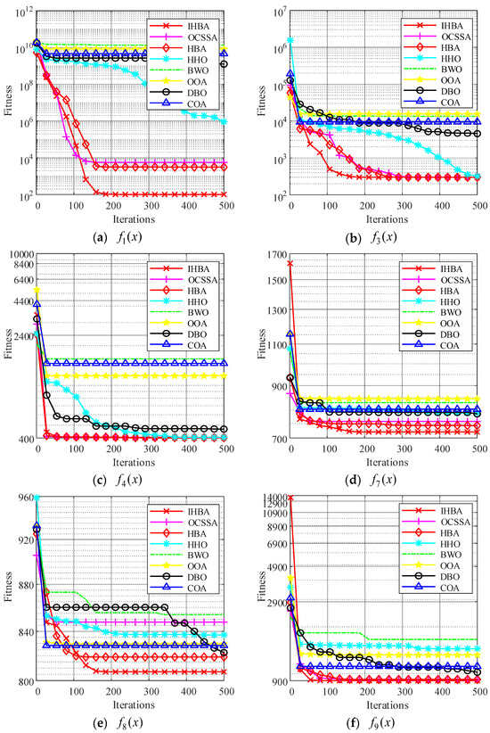
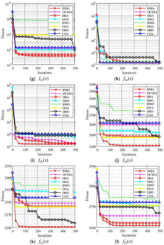
Figure 5.
Twelve classic test functions and convergence curves.
5. Engineering Optimization
To further demonstrate the effectiveness and engineering applicability of the IHBA, it is applied to the bearing fault diagnosis problem. The Variational Mode Decomposition (VMD) algorithm, an adaptive signal decomposition method, uses vital parameters like the penalty factor and the number of modes to enhance performance. The IHBA, a novel metaheuristic algorithm, was effectively applied to optimize the VMD parameters for bearing fault diagnosis, quickly achieving notable results compared to other optimization techniques. Ultimately, VMD was integrated with convolutional neural networks and bidirectional long short-term memory (CNN-BILSTM) to facilitate the diagnosis of bearing faults.
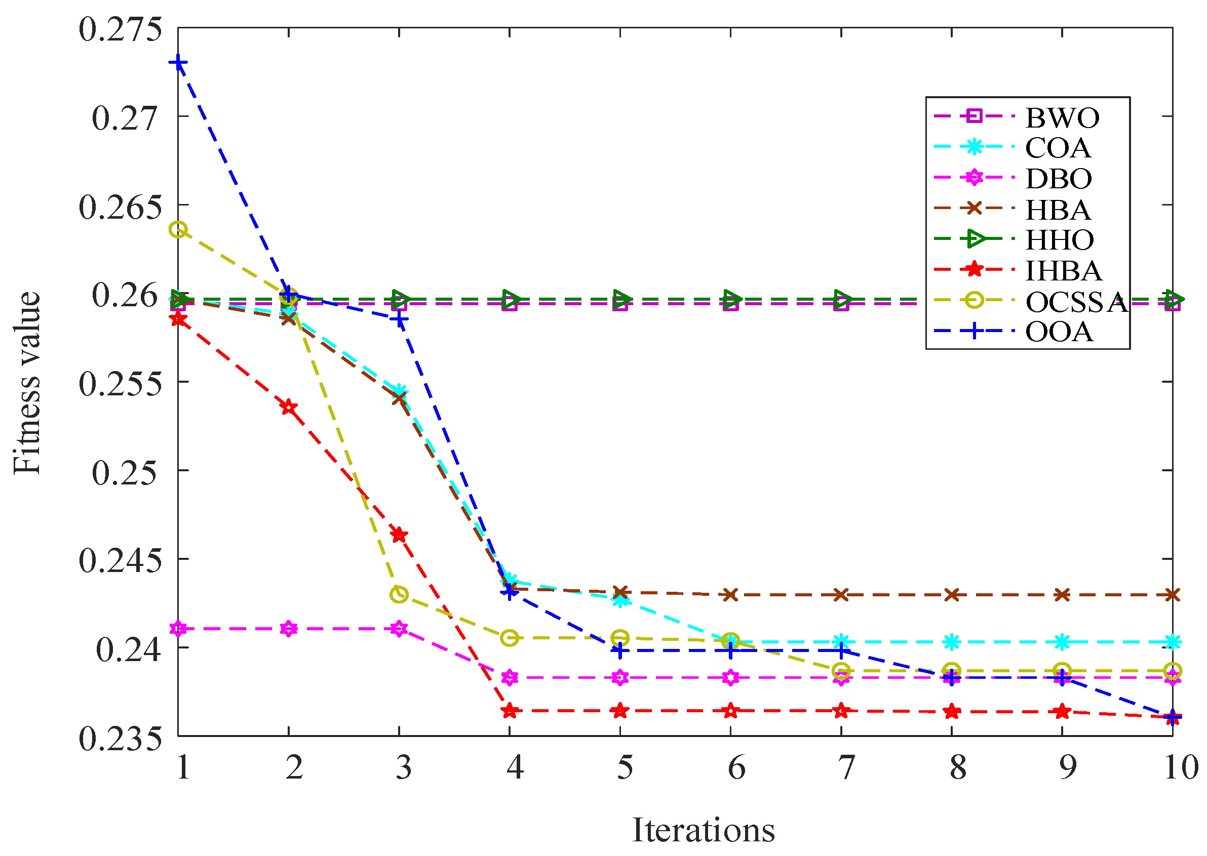
5.1. Optimizing the Parameters of VMD
Different optimization algorithms are used to optimize the VMD parameters, and the adaptability curves are shown in Figure 6. By using the IHBA to optimize the key parameters of VMD, the signal analysis performance can be significantly enhanced. Especially when dealing with complex fault vibration signals, the algorithm in this paper can improve the decomposition quality, reduce the computational complexity, and obtain better accuracy and adaptability.

Figure 6.
Fitness curves for VMD parameter optimization.
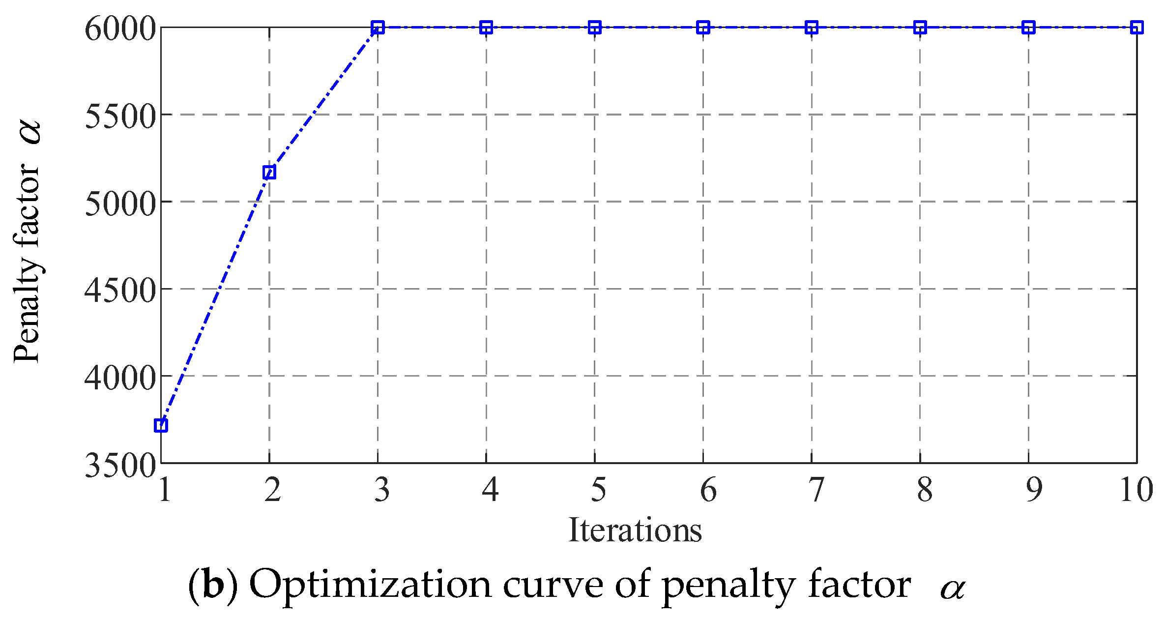
Figure 7 illustrates the convergence curve and parameter variation curve obtained during the optimization of the VMD parameters by the IHBA. As depicted in Figure 8, the convergence process shows that the algorithm tends to stabilize after four iterations, indicating convergence. At this point, the fitness function (minimum permutation entropy) value is 0.2364, with the optimal parameter combinations for the number of decomposition modes () and the penalty factor () being (15, 6000).
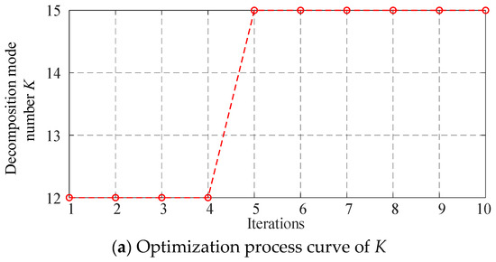

Figure 7.
Optimization process curve of outer ring faulty bearing 0.007.

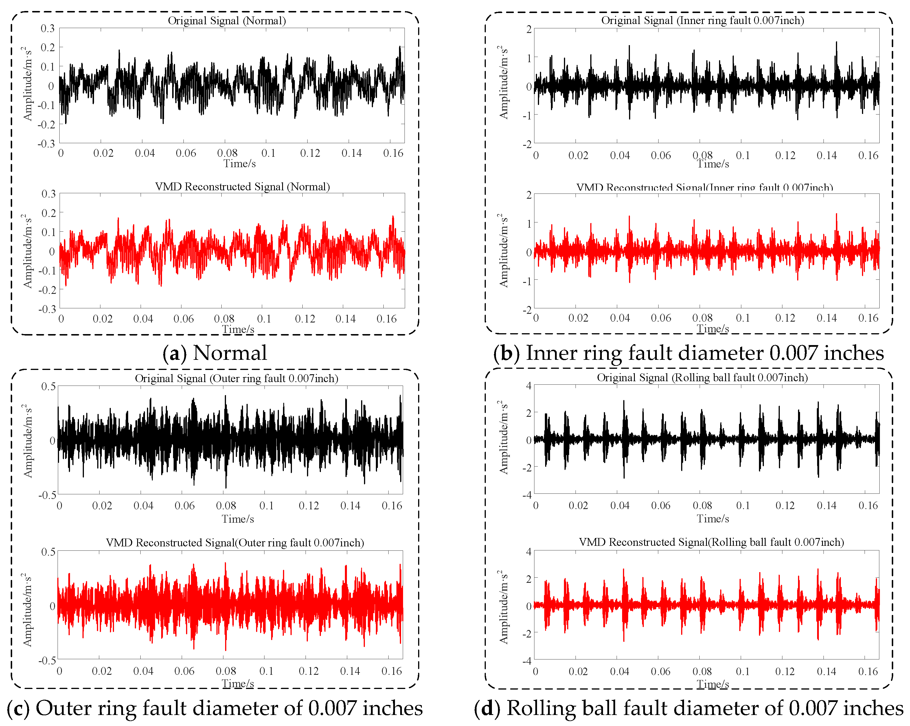
Figure 8.
Time-domain comparison between the original and the reconstructed signals of different faults.
Figure 8a–d shows the time-domain comparison diagrams before and after signal decomposition and reconstruction for a normal bearing and inner ring, outer ring, and rolling body bearing faults, respectively. These figures demonstrate that after optimized VMD reconstruction, the time-domain signals exhibit significant noise reduction, and the impact characteristics of the fault signals become more pronounced.
5.2. Rolling Bearing Fault Diagnosis
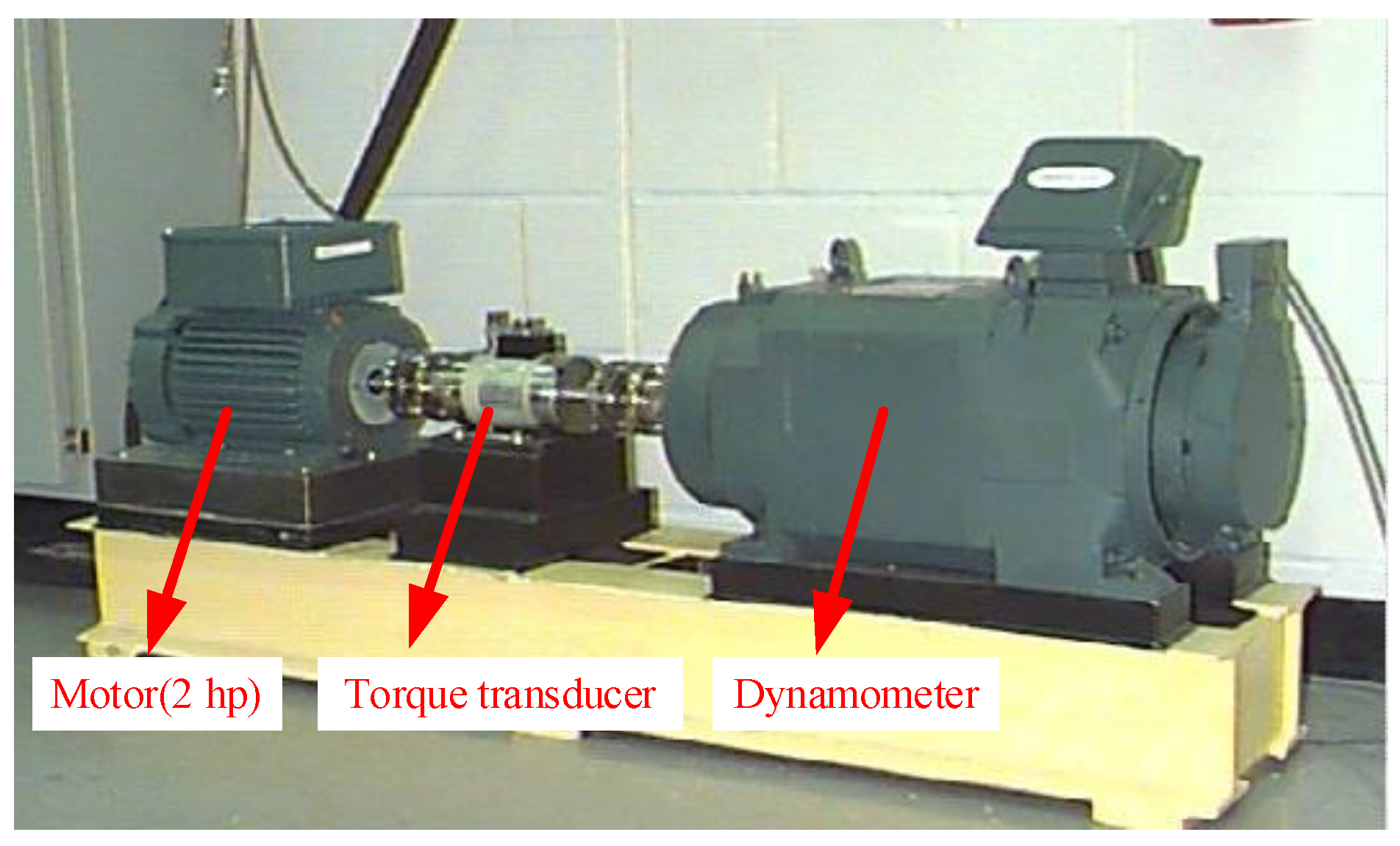
The experimental data used in this study were sourced from the Case Western Reserve University (CWRU) database on motor bearing failures [18]. As shown in Figure 9, a test bench was employed to simulate bearing failures, with a vibration signal sampling frequency of 1024 Hz. The experiment utilized a deep groove ball bearing model SKF6205, with failures simulated via electrical discharge machining (EDM). For diagnostic purposes, 10 fault categories were established, encompassing four types of states as follows: normal bearing, rolling element fault, outer ring fault, and inner ring fault. Each fault state was further categorized based on fault diameters of 0.007 inches, 0.014 inches, and 0.021 inches, resulting in nine distinct states representing varying degrees of failure. The dataset for each fault type consisted of 120 samples, with each sample containing 2048 data points. In the experimental setup, 90 samples were allocated for model training, while 30 samples were reserved for model testing. The division of the fault dataset is detailed in Table 6.

Figure 9.
Bearing fault simulation test bench.
Table 6.
Division results of the fault dataset.
Determining the relevant parameters is crucial in the VMD of the original vibration signals of rolling bearings. Specifically, the number of modal components and the penalty parameter significantly influence the decomposition results. The value of dictates the number of decomposed modal components. If is set too low, under-decomposition occurs, leading to a loss of key information and an inability to extract essential features. Conversely, if is set too high, it results in an excessive number of modal components, causing overlapping center frequencies and making signal feature differentiation difficult. The penalty parameter primarily affects the bandwidth of each modal component, with an appropriate value enhancing the accuracy of the reconstructed signal. In this paper, we propose an approach that optimizes VMD using an IHBA, combining it with a CNN-BiLSTM architecture for the fault diagnosis of motor bearings. This method effectively extracts fault features from the original vibration signals. After the feature extraction process, each of the 10 states is represented by 120 samples, resulting in a 1200 × 9 matrix. Each row of this matrix is labeled with numbers 1–10 to indicate different fault types. The fault diagnosis process, as implemented in this study, is depicted in Figure 10.
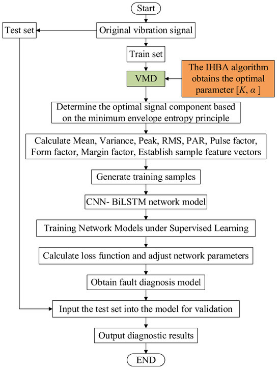
Figure 10.
Based on the IHBA-VMD-CNN-BiLSTM rolling bearing failure prediction flowchart.
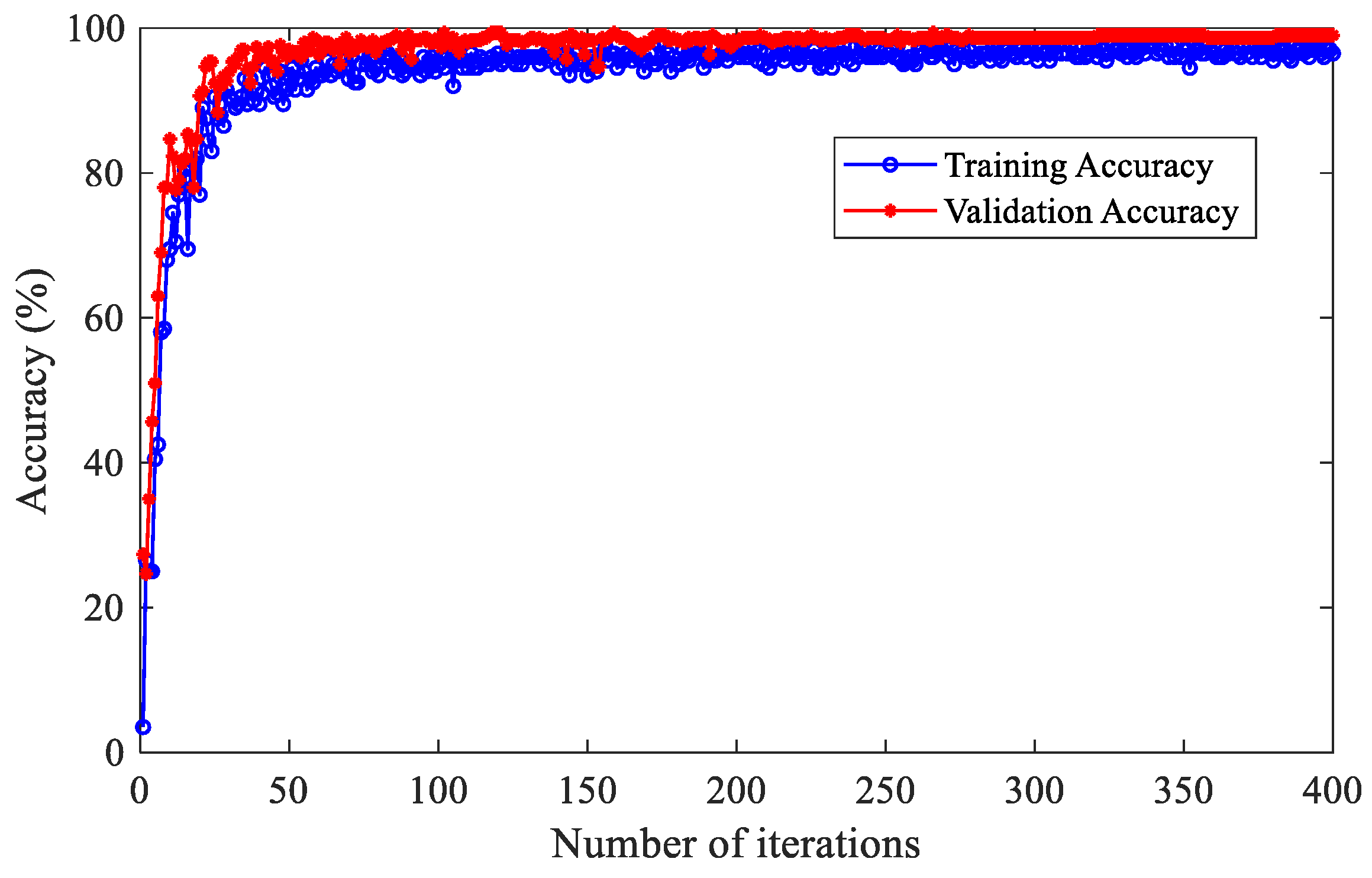
Figure 11 illustrates the accuracy curve of a fault diagnosis model based on IHBA-VMD-CNN-BiLSTM. The model performs excellently during both the training and testing phases, stabilizing after approximately 200 iterations and achieving a testing accuracy of up to 99.67% at 400 iterations.
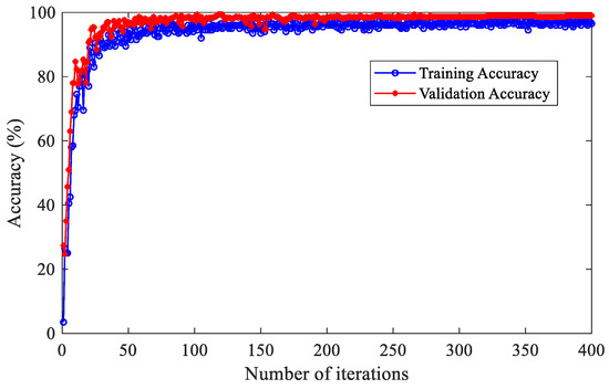
Figure 11.
Accuracy curve of the fault diagnosis model based on IHBA-VMD-CNN-BiLSTM.
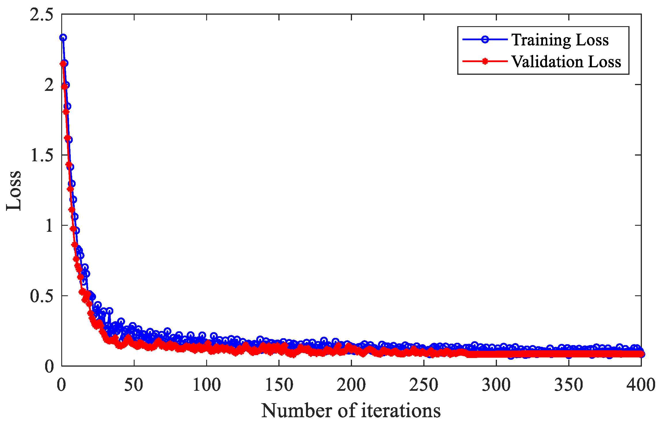
Figure 12 shows the loss function curve of a fault diagnosis model based on IHBA-VMD-CNN-BiLSTM. The model demonstrates excellent performance, with both training and testing losses rapidly decreasing and stabilizing at low values after around 50 iterations.
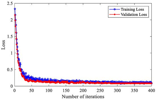
Figure 12.
Loss function curve of the fault diagnosis model based on IHBA-VMD-CNN-BiLSTM.
To evaluate the performance of IHBA-VMD-CNN-BiLSTM, the proposed model is compared with other state-of-the-art (SOTA) models [19]. The confusion matrix and classification results for fault diagnosis are presented in Figure 13. After repeated validation, the IHBA-VMD-CNN-BiLSTM model demonstrates superior performance, achieving a recognition accuracy of 96.7% for normal faults, and 100% for all other fault types. The overall recognition accuracy for the 10 types of faults reaches an impressive 99.34%. Furthermore, the recognition speed of the IHBA-VMD-CNN-BiLSTM model is significantly improved, demonstrating its effectiveness in fault diagnosis.
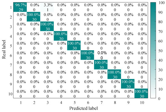
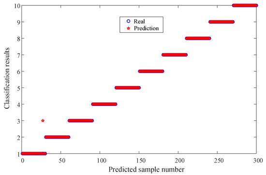
Figure 13.
The accuracy of the test results for the eight methods.
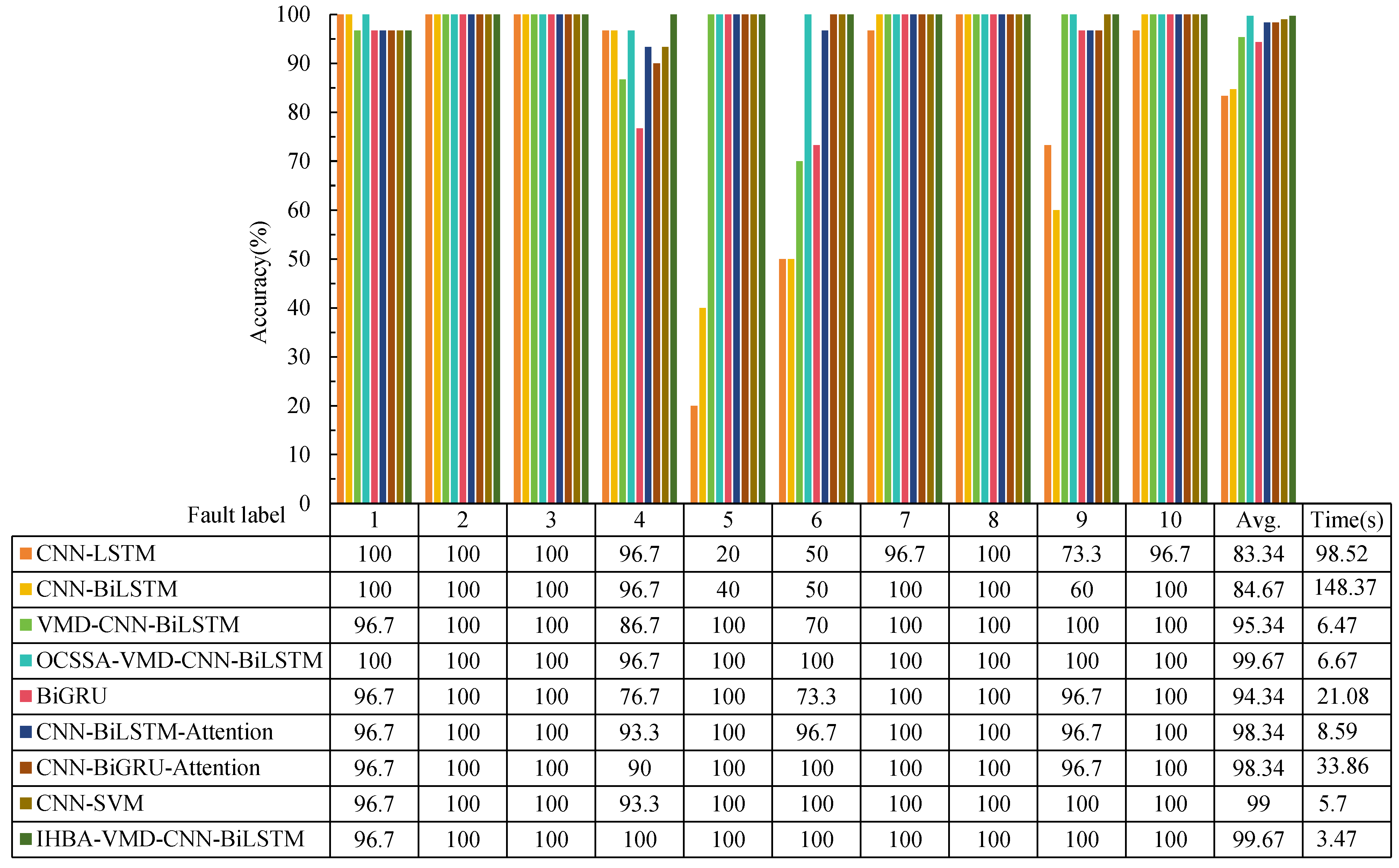
Figure 14 shows the diagnostic accuracy of different experimental methods using the CWRU dataset. The figure presents the accuracy and average processing time of eight different fault diagnosis models applied to 10 types of faults. The IHBA-VMD-CNN-BiLSTM model stands out as the most effective method for fault diagnosis, achieving 100% accuracy for all faults except one, with an overall accuracy of 99.67%. It maintains a very short processing time of 3.34 s, second only to CNN-SVM, which has significantly lower accuracy. Its consistently high accuracy across different fault types demonstrates its robustness. The combination of optimization (IHBA) and advanced feature extraction (VMD) significantly enhances the performance of the CNN-BiLSTM model, making it the best choice for practical applications requiring high accuracy and efficiency in fault diagnosis.

Figure 14.
Diagnostic accuracy of different experimental methods.
6. Conclusions
To address the limitations of the HBA, including poor exploitation, susceptibility to local optima, and insufficient pre-exploration, this study introduces the following key enhancements: cubic chaotic mapping for population diversity, random value perturbation, and repeated random searches to prevent premature convergence and strengthen global optimization. Additionally, an elite tangent search with differential variation accelerates convergence and improves accuracy by leveraging optimal solution information. Simulation and bearing fault diagnosis experiments validate the proposed IHBA’s robustness, stability, and practical applicability, demonstrating its effectiveness in enhancing decomposition quality, reducing computational complexity, and achieving superior precision and adaptability in complex signal analysis tasks. Additionally, experiments on bearing fault diagnosis confirmed the practical applicability of the IHBA in engineering. In summary, the IHBA has performed excellently in enhancing initial population traversal and improving global optimization capabilities. However, its limitations, such as sensitivity to algorithm parameter settings, high computational complexity, need for improvement in convergence speed, and lack of universal validation, also require attention. Future research directions can explore and improve these limitations in depth to further enhance the performance and application scope of the IHBA.
Author Contributions
Conceptualization, H.T.; methodology, C.Y.; software, C.Y.; validation, C.P.; formal analysis, C.Y.; investigation, H.T.; resources, H.T.; data curation, C.P.; writing—original draft preparation, C.Y.; writing—review and editing, H.T.; supervision, project administration, funding acquisition, H.T. All authors have read and agreed to the published version of the manuscript.
Funding
This work was supported by the National Natural Science Foundation of China (51967012), the Gansu Natural Science Foundation (23JRRA1664), and the Innovative Ability Enhancement Project of Gansu Provincial Higher Education (2023A-199), Gansu Province Longyuan Youth Innovation Talent Team Project (310100296012).
Data Availability Statement
The original contributions presented in this study are included in the article. Further inquiries can be directed to the corresponding author(s).
Conflicts of Interest
The authors declare no conflicts of interest.
References
- Alonso-González, M.; Díaz, V.G.; Pérez, B.L.; G-Bustelo, B.C.P.; Anzola, J.P. Bearing Fault Diagnosis With Envelope Analysis and Machine Learning Approaches Using CWRU Dataset. IEEE Access 2023, 11, 57796–57805. [Google Scholar] [CrossRef]
- Ke, Z.; Di, C.; Bao, X. Adaptive Suppression of Mode Mixing in CEEMD Based on Genetic Algorithm for Motor Bearing Fault Diagnosis. IEEE Trans. Magn. 2022, 58, 1–6. [Google Scholar] [CrossRef]
- Xue, J.K.; Shen, B. A novel swarm intelligence optimization approach: Sparrow search algorithm. Syst. Sci. Control Eng. 2020, 8, 22–34. [Google Scholar] [CrossRef]
- Huang, K.W.; Wu, Z.X.; Jiang, C.L.; Huang, Z.H.; Lee, S.H. WPO: A Whale Particle Optimization Algorithm. Int. J. Comput. Intell. Syst. 2023, 16, 1–16. [Google Scholar] [CrossRef]
- Trojovsky, P.; Dehghani, M. Pelican Optimization Algorithm: A Novel Nature-Inspired Algorithm for Engineering Applications. Sensor 2022, 22, 855. [Google Scholar] [CrossRef]
- Mirjalili, S.; Mirjalili, S.M.; Lewis, A. Grey wolf optimizer. Adv. Eng. Softw. 2014, 69, 46–61. [Google Scholar] [CrossRef]
- Heidari, A.; Mirjalili, S.; Faris, H.; Mafarja, M. Harris hawks optimization: Algorithm and applications. Future Gener. Comput. Syst. 2019, 97, 849–872. [Google Scholar] [CrossRef]
- Hashim, F.A.; Houssein, E.H.; Talpur, K.; Mabrouk, M.; Al-Atabany, W. Honey badger algorithm: New metaheuristic algorithm for solving optimization problems. Math. Comput. Simul. 2022, 192, 84–110. [Google Scholar] [CrossRef]
- Abasi, A.K.; Aloqaily, M. Optimization of CNN using modified honey badger algorithm for sleep apnea detection. Expert Syst. Appl. 2023, 229, 120484. [Google Scholar] [CrossRef]
- Zhou, C.; Gao, B.; Yang, H.; Zhang, X.; Liu, J.; Li, L. Junction temperature prediction of insulated-gate bipolar transistors in wind power systems based on an improved honey badger algorithm. Energies 2022, 15, 7366. [Google Scholar] [CrossRef]
- Düzenli, T.; Onay, F.K.; Aydemir, S.B. Improved honey badger algorithms for parameter extraction in photovoltaic models. Optik 2022, 268, 1169731. [Google Scholar] [CrossRef]
- Xue, J.; Shen, B. Dung beetle optimizer: A new meta-heuristic algorithm for global optimization. J. Supercomput. 2023, 79, 7305–7336. [Google Scholar] [CrossRef]
- Mohammad, D.; Zeinab, M.; Eva, T.; Pavel, T. Coati Optimization Algorithm: A new bio-inspired metaheuristic algorithm for solving optimization problems. Knowl.-Based Syst. 2023, 259, 110011. [Google Scholar]
- Dehghani, M.; TrojovskýSec, P. Osprey optimization algorithm: A new bio-inspired metaheuristic algorithm for solving engineering optimization problems. Engine Automot. Eng. 2022, 8, 1126450. [Google Scholar] [CrossRef]
- Zhong, C.; Li, G.; Meng, Z. Beluga whale optimization: A novel nature-inspired metaheuristic algorithm. Knowl.-Based Syst. 2022, 251, 109215. [Google Scholar] [CrossRef]
- Yong, C.; Ting, H.; Peng, C. Enhancing sparrow search algorithm with OCSSA: Integrating osprey optimization and Cauchy mutation for improved convergence and precision. Electron. Lett. 2024, 60, e13127. [Google Scholar] [CrossRef]
- Layeb, A. Tangent search algorithm for solving optimization problems. Neural Comput. Appl. 2022, 34, 8853–8884. [Google Scholar] [CrossRef]
- Available online: https://engineering.case.edu/bearingdatacenter (accessed on 1 October 2024).
- Yong, C.; Guangqing, B. Enhancing Rolling Bearing Fault Diagnosis in Motors using the OCSSA-VMD-CNN-BiLSTM Model: A Novel Approach for Fast and Accurate Identification. IEEE Access 2024, 12, 78463–78479. [Google Scholar]


Disclaimer/Publisher’s Note: The statements, opinions and data contained in all publications are solely those of the individual author(s) and contributor(s) and not of MDPI and/or the editor(s). MDPI and/or the editor(s) disclaim responsibility for any injury to people or property resulting from any ideas, methods, instructions or products referred to in the content. |
© 2025 by the authors. Licensee MDPI, Basel, Switzerland. This article is an open access article distributed under the terms and conditions of the Creative Commons Attribution (CC BY) license (https://creativecommons.org/licenses/by/4.0/).