Article

Application Research of Vision-Guided Grinding Robot for Wheel Hub Castings

1
Shaanxi Key Laboratory of Advanced Manufacturing and Evaluation of Robot Key Components, Baoji 721016, China
2
School of Mechanical Engineering, Baoji University of Arts and Sciences, Baoji 721016, China
*
Author to whom correspondence should be addressed.
Processes 2025, 13(1), 238; https://doi.org/10.3390/pr13010238
Submission received: 23 December 2024 / Revised: 8 January 2025 / Accepted: 11 January 2025 / Published: 15 January 2025

Abstract

:
The combination of vision and robotic grinding technology provides robots with “visual perception” capabilities that enable them to accurately locate the area to be ground and perform the grinding tasks efficiently. Based on the rough grinding requirements for wheel hub burrs proposed by a casting company, this paper investigates the application of a vision-guided grinding robot in treating burrs on wheel hub castings. First, through vision system calibration, the conversion from pixel coordinate system to robot base coordinate system is implemented, thus ensuring that the subsequently extracted burr point coordinates can be correctly mapped to the robot’s operational coordinate system. Next, the images of the burrs on wheel hub castings are collected and processed. All the burr points are extracted by applying image algorithms. In order to improve grinding accuracy, a height error compensation model is established to adjust the coordinates of the 2D-pixel points; the coordinate error after compensation was reduced by 58.33%. Subsequently, the compensated burr point trajectories are optimized by utilizing an intelligent optimization algorithm to generate the shortest grinding path. Through experimental analysis of the relationship between spindle speed and surface roughness, a grinding trajectory simulation model is constructed, and the simulation results are integrated into the robot system. Finally, actual wheel hub burr grinding experiments are performed to validate the effectiveness and practicality of the proposed solution.

1. Introduction

China’s foundry industry has a broad market. Replacing manual grinding with automated robotic grinding has become an inevitable trend with the maturity and popularization of industrial robot technology. The main defect in automotive wheel hub casting is burr. At present, most enterprises utilize a combination of robotic rough grinding and manual finishing. However, the existing robotic grinding programs are fixed and only suitable for the complete grinding of certain workpieces, resulting in a waste of resources. Compared with the above grinding methods, intelligent grinding based on vision-guided industrial robots possesses several advantages: (1) Simplified operation and low labor intensity. For standardized castings, long-term and large-scale automated grinding can be achieved by demonstrating vision-guided path planning. (2) Higher work efficiency. A vision system can accurately locate burrs and optimize grinding trajectories, shorten grinding time and meet the demands of efficient grinding. (3) Better grinding consistency. Robotic grinding is performed using a grinding process determined through multiple experiments. With consistent grinding power and high precision, it avoids the quality variations that may be brought by manual operations. Automatic grinding of automobile wheel hub castings can not only enhance product quality and bring benefits to enterprises but also effectively ensure worker safety and align with the development trends of new and old kinetic energy conversion, as well as meet the high-quality development needs of the manufacturing industry [1]. By integrating industrial robots with machine vision technology to extract burr location points and guide the robot to precisely grind the wheel hub burrs, this paper addresses the rough grinding requirements of wheel hub burrs in a casting enterprise.
For grinding robot technology, foreign grinding robot technology dates back to the 1950s when industrial developed countries began applying automatic control technology to grinding. By the end of the 1970s, Japan began research into mechanical arm polishing and grinding. Subsequently, the United States, Germany, South Korea and other countries conducted extensive research on factors such as grinding force, speed, feed rate, path, material removal rate, etc. Moreover, they established mathematical models of grinding force and developed related grinding equipment, thus laying the foundation for automated grinding. For example, Villagrossi et al. from Danieli Metallurgical Equipment Co., Ltd. in Italy [2] have developed a grinding robot for hard materials that optimizes the trajectory by means of single-axis force sensor feedback in order to avoid elastic effects on the system structure. In recent years, domestic enterprises, universities, and colleges have increasingly focused on the research and development of grinding robots. Du from Dalian University of Technology [3] designed a multi-axis robot processor that effectively avoided vibration and collision and achieved good polishing results by using a flexible end device and force feedback sensors to polish titanium alloy surfaces. Hong et al. from the National Center University [4] integrated robotic arms into the electrochemical mechanical polishing of titanium alloys and improved surface smoothness and corrosion resistance with a new grinding head. Researchers from Universidad Politecnica de Valencia applied the theory of topology to optimize the robot path and reduce the path length during the grinding process through trajectory planning [5,6]. Guo et al. [7] from Chang’an University developed a robot for removing welds at the ends of welded pipes and verified its superiority and planning reliability. While researching the grinding of sheet metal, Sean et al. [8] calculated the contact area using the Hertz theory and adopted the finite element method to solve the problems of deformation caused by the contact force, thus ensuring a uniform polishing of the surface.
For vision detection technology, it is required to capture images of the wheel hub castings to be ground first, then extract the coordinates of the burr points combined by vision detection technology and transformed from pixel coordinates to robot coordinates based on the results of vision calibration, thus guiding the robot to complete the grinding operation. Foreign machine vision research began in the 1960s. Initially, it was not widely used in actual production due to low equipment accuracy and large measurement errors. As the hardware upgraded and digital imaging technology developed, machine vision gradually overcame its limitations. In contrast, the development of machine vision in China has been slower. Machine vision companies did not emerge until the early 1990s when robotic grinding was gradually integrated with vision systems. For instance, Shi et al. from Guangdong University of Technology [9] introduced a 3D vision system, extracted machining path points and successfully integrated them into an automatic grinding system. Liu et al. [10] developed an autonomous robotic polishing system based on sensor signal processing and carried out intelligent defect detection with the combination of machine vision and force sensors. A new type of polishing robot for precision machining of large mold surfaces was developed by Wang et al. from Jilin University [11] by combining machine vision with mobile robots. This robot is designed for the precision finishing of large mold surfaces, using vision positioning for grinding operations. In addition, in order to solve robot trajectory planning problems, many researchers have introduced intelligent optimization algorithms. For example, Hua et al. [12] used an evolutionary particle swap optimization algorithm to plan the trajectory of a painting robot and verified its effectiveness. Zhang et al. [13] designed a constant-force end effector for precision machining with magnetorheological fluid, which effectively compensates for positioning errors and maintains the stability of the polishing process. A traditional ant colony algorithm is mainly used to solve the problem of traveling quotient, but it has certain limitations, Cheng [14] used the improved ant colony algorithm to optimize the path, mainly determine the influencing factors of multi-objective planning model, improve the ant colony algorithm, using hierarchical analysis (AHP) the path length, travel time and traffic flow into comprehensive weight influence factor. The travel time (376 s) of the optimal path obtained by the improved colony algorithm is significantly shorter than the travel time of the basic colony algorithm (416.3 s). To address the challenges posed by the artifact section dataset, Lin [15] used an innovative ant colony optimization algorithm that enhances the trajectory of the tool. By treating the optimization of the motion path as the travel quotient problem (TSP), the ant colony algorithm arranges the versal order of the clusters according to the center of the cluster and then calculates the shortest path within each cluster. Finally, the significant enhancement of the movement path significantly improves the work efficiency.
At present, the grinding of the burr of the wheel hub casting tends to be polished by combining vision and force sensors, mainly to polish the overall outline of the wheel hub and the grinding is not targeted; based on this, it is proposed to use vision to find the burr point and then seek the optimal grinding sequence of the burr point through the intelligent optimization algorithm, and finally all the burr points on the wheel hub can be polished in a targeted manner, without the need to polish the overall profile of the wheel hub, to improve the grinding efficiency. Based on the above analysis, in response to the wheel hub burr grinding needs of a foundry, this paper integrates vision technology with robots to complete the rough grinding of wheel hub burrs. First, the vision system extracts the wheel hub 2D image and performs burr coordinate extraction, the main work outline is shown in Figure 1. Then, a height compensation model is applied to correct the coordinates and improve the grinding accuracy since the height difference of the burrs will cause the 2D coordinates to deviate. Next, the grinding trajectory is designed to improve efficiency using an intelligent optimization algorithm. Finally, a simulation model is set up, and experiments are conducted to verify the relationship between the spindle speed and the roughness and, finally, to determine the effective grinding parameters. The experiments show that the system can grind wheel hub burrs quickly, accurately and effectively. In actual grinding operations, it can liberate a certain amount of labor force, which can be converted to robots for grinding, thereby shortening the grinding time and improving the grinding quality.

2. Vision System Calibration

Vision system calibration is a conversion job that realizes the transformation from pixel coordinates to robot basal coordinates. It mainly involves three calibrations, namely, camera, hand–eye calibration, and tool–hand calibration. Among them, camera calibration is aimed at obtaining the camera’s internal parameters (such as the focal length and the position of the optical center) and the external parameters. Hand–eye calibration is utilized to estimate the transformation relationship between the end effector of the mechanical arm and enable applications such as visual robot navigation and precise positioning. Tool–hand calibration is the process of determining the position and orientation of the industrial robot end tool (such as a welding torch and grinding head) relative to the end of the mechanical arm, requiring both position and orientation calibration.
Determining the camera’s internal and external parameters is the main purpose of camera calibration. Internal parameters include focal length, center of gravity and distortion coefficients. The external parameters describe the position and orientation of the camera in the world coordinate system, where the position is the specific location of the camera in the world coordinate system. Camera calibration methods mainly include traditional calibration, self-calibration, and Zhang’s method [16]. Zhang’s method is adopted in this paper using a checkerboard calibration plate measuring 200 × 200 mm, consisting of 7 × 7 alternating black and white squares, each measuring 18 × 18 mm. With an accuracy of ±0.05 mm, the chessboard is made of alumina to avoid glare. The chessboard selected for the experiment is shown in Figure 2.
When grinding wheel hub castings, the grinding head is mounted at the end of the mechanical arm, and the end coordinate system is converted to the center of the grinding head. Tool–hand calibration is required to achieve accurate grinding, and its calibration involves a six-point method and a four-point method. The six-point method offers higher calibration accuracy. Although the operation is complex, it provides extensive spatial information, making it more sensitive to error. Therefore, in this study, the six-point method is chosen to calibrate the tool coordinate system.
Hand–eye calibration is used to obtain the 3D rigid transformation (pose) between the robot and the camera [17]. It converts the pose information of the object captured by the camera in the world coordinate system into spatial coordinates in the base coordinate system. Eye-to-hand configuration is suitable for dynamic environments and scenarios that require greater robot flexibility, as it allows the camera and the mechanical arm to move independently. Eye-in-hand configuration fixes the camera to the end of the mechanical arm, ideal for high-precision tasks, as shown in Figure 3.
First, particulate matters that can damage the camera lens are inevitable when grinding castings for automotive wheel hubs. Then, the mechanical arm needs to perform grinding in different poses due to the uneven distribution of burrs on the wheel hub. Given these considerations, the eye-to-hand configuration is more suitable for the actual grinding process.
The camera lens must be level with the end face of the wheel hub in order to capture the full contour image of the wheel hub and clear burr images. At the same time, the actual camera and wheel hub placement position is shown in Figure 4 to allow the mechanical arm to grind the wheel hub effectively and to prevent grinding debris from damaging the camera lens.

3. Burr Coordinate Extraction and Position Compensation

This chapter not only involves extracting defect position information from the captured burr images but also involves converting 2D pixel coordinates into robot-readable robot coordinates. There is a proportional relationship between height and lens magnification because the wheel hub is a casting with 3D feature information. Based on this relationship, a height error compensation model is established to eliminate the effect of height differences on the inaccurate positioning of burr points.

3.1. Burr Coordinate Extraction Based on Image Difference

3.1.1. Image Filtering and Burr Point Extraction

Following the analysis above, the image of the wheel hub casting captured by the vision camera is shown in Figure 5.
Considering that all the burr points need to be segmented, gray processing, image filtering, histogram equalization, edge detection and image difference comparison and image difference comparison operators are adopted to perform image processing. There are three methods for gray processing involving maximum value, mean value and weighted mean value. The corresponding formulas are shown in (1) to (3):
Gray i ,   j =   max   { R i ,   j ,   G i ,   j ,   B i ,   j }
Gray i ,   j = { R i ,   j + G i ,   j + B ( i ,   j ) 3 }
Gray i ,   j = 0.299     R i ,   j + 0.578     G i ,   j + 0.114     B i ,   j
where Gray(i, j) is the final gray value and R(i, j), G(i, j), and B(i, j) are the brightness values of the three color components in the original image.
Filter processing can smooth the image and remove noise points. Median filtering and mean filtering are the primary filtering methods. In contrast to median filtering, mean filtering calculates the average gray value of the pixels within a certain neighborhood and assigns this average value to the center pixel in the filtered image. The formula is shown in (4):
g x ,   y = 1 M   i ,   j     S   f ( i ,   j )
where g(x, y) is the pixel value after mean filtering, f(i, j) is the pixel value at position (i, j) in the original image, S is the neighborhood of the current pixel (x, y), and M is the total number of pixels in the neighborhood.
Filter processing can effectively highlight the location of burrs, but the original image often has a local uneven brightness. Histogram Equalization (H E) enables significant improvement in image contrast and enhances texture features. The main principle of H E is to transform the original histogram into a uniform distribution and extend the dynamic range of gray values, thus improving contrast, as shown in Figure 6.
HE can effectively represent the shape of burr defects. However, image enhancement operators are needed to process the burr edge information for subsequent image difference comparison and accurate burr defect extraction. The core idea of image edge detection is based on gradient, which measures the rate of change of image intensity. Gradients are large at edges where gray values change significantly and small in smooth areas. Since images are 2D discrete data, the gradient at the point (x, y) can be calculated by generalizing the partial derivative method of continuous functions, as shown in Figure 7.
If point A is located on an edge, then the direction of the gradient at point A is perpendicular to the direction of the edge. This means that at points where there are significant changes in gray level, the direction of the gradient will be perpendicular to the edge. Hence, the core of edge detection is gradient. In order to enhance the edge information of burrs, it is necessary to select appropriate edge detection operators to extract the burrs, where common edge detection operators include Roberts operator edge detection, Sobel operator edge detection, Prewitt operator edge detection, and Canny edge detection. Among them, the Sobel operator has a smoothing effect on noise and can provide more accurate edge direction information. Its disadvantage is that the edge positioning accuracy is not high enough. The Roberts operator detects the edge by reaching an extreme value at the edge. However, its disadvantage is that it is sensitive to noise and easily produces pseudo edges. The Prewitt operator has a smoothing effect on the noise and can remove some pseudo edges. The disadvantage is that the implementation method is similar to the Sobel operator, but the positioning accuracy is not as good as the Roberts operator. Compared with the Prewitt operator and Roberts operator, the Sobel operator has the advantages of high positioning accuracy and small operation amount. The Sobel operator was therefore chosen for the detection of the burr point edges.
After processing with the Sobel operator, the images are subjected to a difference comparison. Given two hub images, ImageEquHisto1 and ImageEquHisto, with known pixel coordinate values (x, y) for each point, subtracting one image from the other removes the common parts and retains the differences. These differences correspond to the coordinate information of the burr points in the burr image. The mathematical expression is given in (5):
ImageAbsDiff x ,   y = ImageEquHistol x ,   y ImageEquHisto x ,   y
where: ImageAbsDiff(x, y) represents the pixel value in the resulting image, corresponding to the pixel value at (x, y) in the burr image.

3.1.2. Circle Center Coordinate Recognition Based on the HCD Algorithm

The extracted burr pixel points are represented in 2D coordinates, whereas the wheel hub casting has a 3D contour. Each burr point has different height information, and the distance between the camera and each burr point varies, resulting in changes in the camera’s working distance. This variation will cause a displacement of the 2D coordinates so as to affect the positioning accuracy of the burr points. Therefore, compensating for the height error is required to mitigate the effect of height differences on the 2D coordinates. To achieve this, this paper uses image moments to extract the center coordinates of the calibration plate. A height error compensation model is established. Meanwhile, the Hough transform is used to extract the centroid coordinates of the burr points to verify the accuracy of the height error compensation.
The moments of an image region [18] represent the normalized grayscale image function as the probability density of a 2D random variable, which is typically stored in a 2D array. In image processing, suppose the image is a thin plate with uneven quality density; then, the grayscale distribution function f(x, y) refers to the density distribution of the thin plate at position (x, y). Origin moment M00 represents the sum of all pixel values, while the first-order original moments (M10 and M01) are used to calculate the centroid coordinates of the image. Hence, the centroid coordinate (x0, y0) can be calculated through first-order moments. The formulas are shown in (6) and (7):
x 0 = m 10   m 00
y 0 = m 01   m 00
To extract circles in the height error compensation experiment, The Hough Circle Detection (HCD) algorithm is adopted. HCD algorithm seeks circle parameters in the accumulator space by applying the Hough transform to identify circular objects in the image [19], as shown in Figure 8.
x i a 2 + y i b 2 = r 2  
a x i 2 + b y i 2 = r 2
In image space, multiple points on a circle can be obtained by Formula (8). This is then transformed into multiple corresponding circles in parameter space, as shown in Formula (9). The center of the circle in parameter space corresponds to the intersection of these circles in image space. Using this principle, it is possible to obtain the coordinates of the centers of the nine circles in the image.

3.1.3. 2D Pixel Coordinate Position Compensation Based on Height Linear Interpolation

The extracted burr pixel points are represented in 2D coordinates, whereas the wheel hub casting has a 3D contour. In order to reduce the effect of height variations on the 2D coordinates, it is necessary to perform camera height error compensation due to the different height information of different burr points. The camera height error refers to the difference between the expected height of the camera and the actual height of the object or scene. This kind of error may cause changes in camera perspective, magnification and image distortion, thus affecting measurement accuracy and image quality. This error is most common when detecting or measuring workpieces with various height characteristics. For wheel hub castings, the camera is fixed at a constant focal length and mounted on the outside. Therefore, changes in the distance between the camera and the object cause variations in optical magnification, resulting in errors in the r and v coordinates of the image, which in turn affect the extraction of contour edges and grinding effects. To overcome this, camera height compensation is required to correct height-related burr coordinate errors. The pixel coordinates of the circle centers on the calibration plate at different heights were obtained through experimental measurements and calibration procedures, as shown in Figure 9.
From Figure 9, it is clear that the pixel coordinates of circle centers at 0 mm height differ from those at other heights. In practice, the pixel coordinates of the nine points should not vary significantly with changes in height because the position of the calibration plate does not change significantly. However, as shown in Figure 9, except for the height of 0 mm, the circle center coordinates have changed at the other five heights. The magnitude of this change increases with the height difference. This indicates that height differences do affect the camera’s coordinates. As the height changes, the error gradually increases.
The relationship between the image size of the object on the camera sensor and the actual size of the object is called the optical magnification of the camera. The calculation Formula (10) for optical magnification is:
N =   f     d  
where f is the focal length of the lens, and d is the distance from the object to the lens.
The relationship between height and magnification is shown in Table 1.
Fitting the measurement results shows that there is a positive linear relationship between height and image magnification, as shown in Figure 10. Therefore, the actual image size should decrease proportionally as the height increases. The proportional relationship is expressed by Formula (11):
K = 0.0049     Δ Z
where ΔZ is the height difference between the calibration plane and the corresponding height of the contour point of the aluminum alloy die casting.
The edge coordinate points can be compensated for height errors using the proportional coefficient K obtained from the height of the aluminum casting. As shown in Formulas (12) to (14), since the edges of the aluminum casting have different heights relative to the calibration plane, the actual image pixel coordinates (r2, v2) have the following relationships with the corresponding heights:
Δ Z = Z 1 Z 0
r 3 = K r 2 r 0 + r 0
v 3 = K v 2 v 0 + v 0
where Z0 refers to the height of the calibration plane, and (r3, v3) refers to the compensated coordinates of the burr points.
The total height of the wheel hub casting is 200 mm, with burrs mainly distributed in the top layer, between the spokes and in the intermediate area between these two areas. Specifically, the top layer of the wheel hub casting is 200 mm above the calibration plane, the spokes are 140 mm above the calibration plane, and the height difference between the top layer and the spokes is 60 mm. To eliminate coordinate inaccuracies caused by the change in distance between the camera and the calibration plane due to height differences, the burr coordinates of the wheel hub casting can be compensated based on the concept of height error compensation. This compensation method can improve the accuracy of burr position extraction by effectively reducing coordinate deviations caused by height differences.

4. Path Planning for Burr Points to Be Ground

4.1. Location of Burr Defects on the Wheel Hub

In practice, there are a total of 11 burr points. The positions of the burrs are mutually independent, and the distribution is not particularly uniform, mainly concentrated in the central area of the image. Among them, eight burr points are at the same height. The remaining four burr points are almost at another different height, with a height difference of 6 cm, as shown in Figure 11.
During the actual grinding process, the grinding head at the end of the mechanical arm traverses the 11 burrs sequentially to complete the wheel hub burr grinding. We can conceptualize the manipulator end as a ‘salesman’ and the burrs as ‘cities’. The grinding path optimization problem can be treated as a traveling salesman problem (TSP), thus improving the grinding efficiency. For 11 burrs, there are 3,628,800 possible paths. Obviously, using intelligent optimization algorithms to find the optimal path is essential in actual production.

4.2. Grinding Path Planning Based on Enhanced ACO Algorithm

4.2.1. Original ACO Algorithm and Improvement Strategies

The ant colony optimization (ACO) algorithm is one of the classic algorithms. It is representative of solving similar path planning problems, so we conduct algorithm design based on the ACO algorithm. Traditional ant colony optimization algorithm defines the heuristic function as the inverse of the Euclidean metric between the current node i and the next node j. This heuristic function easily guides the ants in choosing the nearest node. However, for wheel hub burrs, both horizontal and vertical distances must be taken into account. Therefore, in this paper, horizontal distance, vertical distance and smoothness of path transitions are considered to construct a heuristic function by introducing multiple objectives. A quasi-three-dimensional multi-objective heuristic function is formulated as shown in Formula (15):
f i j t = w 1   d i j t + w 2   ϕ i j t
where w1 and w2 are weight coefficients, dij(t) refers to the quasi-three-dimensional path function, and φij(t) represents the path smoothness evaluation function. Its expression is shown in (16):
d i j t = 1 w 3 S i j + w 4   S j g
In the formula, Sij is the Euclidean metric between the current node i and the next node j, and Sjg is the Euclidean metric between the next node j and the target node g. w3 and w4 are weight coefficients. The coordinates of the current node i are (x1, y1, z1), the next node j are (x2, y2, z2), and the target node g are (x3, y3, z3). The Euclidean metrics Sij and Sjg are calculated using Formulas (17) and (18), respectively:
S i j = x 2 x 1   2 + y 2 y 1 2 + z 2 z 1 2
S j g = x 3 x 2 2 + y 3 y 2 2 + z 3 z 2 2
The Euclidean metric between the next node j and the target node g is introduced to prevent the ant colony optimization algorithm from getting trapped in local optima. The algorithm can incorporate global information when selecting the next node and avoid local optimization by adjusting the weight factors. In addition, the algorithm is better suited to the 3D nature of wheel hub castings by incorporating the position information of the z-axis to ensure that both horizontal and vertical distances are considered.
The path smoothness evaluation function φij(t) is expressed in Formula (19):
ϕ i j t = 360 ° ϕ 1 + ε   + 360 ° ϕ 2 + ε  
In the formula, θi1 and θi2 are the angles formed by the line connecting node i and the previous node i-1 projected onto the x-axis and y-axis, respectively. Similarly, θj1 and θj2 are the angles formed by the line connecting node j and node i. The differences between θi1 and θj1 and between θi2 and θj2 are denoted as φ1 and φ2, respectively. Ε refers to the constant, ensuring that the expression remains meaningful in practical applications. As illustrated in Figure 12, the sum of these angle differences φi represents the turning angle for the ant’s next move. A smaller value of the turning angle φij indicates a smoother path.
To sum up, the improved heuristic function incorporates both quasi-three-dimensional path length evaluation and path smoothness evaluation; the influence of height information will be considered in the actual process of seeking the optimal polishing path in order to make the trajectory pass smoother. This ensures that the ant colony optimization algorithm can find an efficient and smooth path for grinding wheel hub burrs in a 3D environment.
During the actual grinding process, safety points are assigned to each burr point to ensure safe grinding head movement and collision avoidance. The principle of safety point setting is to maintain the horizontal position of the burr point while adjusting its height to create the appropriate safety point. As a result, when the grinding head moves from one burr point to another, it has to pass through the respective safety points.
In the path planning process, the grinding path is first determined by means of the intelligent optimization algorithm. The safety points are then inserted into the optimized path. On this basis, the optimal path is selected by calculating the total distance of the path, including the safety points. This approach ensures that the grinding process is both safe and smooth.

4.2.2. Principles of Multiple Algorithm Planning and Basic Parameter Settings

Genetic Algorithms (GA) simulate the selection process in nature to generate new tentative solutions for mutation operators such as crossover and variation (mutation) [20]. Initially, phenotype-to-genotype coding is required. Individuals are selected based on fitness after the initial population is generated. Through successive generations of crossover and mutation, the algorithm evolves to produce increasingly optimized solutions, eventually reaching an approximate optimal solution. Simulated Annealing (SA) is a random search algorithm inspired by the physical process of annealing. It optimizes solutions by gradually reducing the temperature. It starts with a randomly generated solution [21], which was first proposed by Metropolis et al. Particle Swarm Optimization (PSO) is a metaheuristic algorithm [22] inspired by swarm intelligence. It simulates the foraging behavior of groups of animals, in which the particles move around in the search space to find the optimal solution to the problem.
The basic parameter settings for the ant colony optimization algorithm used in this study are detailed in Table 2:

5. Establishment of the Simulation Platform and System Experiment

5.1. Robot Vision System Calibration Experiment

Images of a checkerboard in different configurations are required for Zhang’s calibration method. As shown in Figure 13, the checkerboard was placed in 30 different configurations in this paper.
The camera parameters obtained through MATLAB calibration are presented in Table 3 and Table 4.
The images of the calibration plate were acquired, and the nine points on the calibration plate were selected using the threshold segmentation method, as shown in Figure 14.
Through HomMat2D transformation, the transformation matrix parameters between the camera and the robot can be obtained, as shown in Table 5. Here, ‘a’ and ‘e’ define the scale factors along the x-axis and y-axis, respectively. ‘b’ and ‘d’ represent the rotational components, while ‘c’ and ‘f’ represent the translate components. ‘c’ refers to the translation along the x-axis and ‘f’ refers to the translation along the y-axis.
Based on the six parameters, pixel coordinates can be converted into robot coordinates. As a monocular camera was used in this project, only (x, y) coordinate information can be obtained by hand–eye calibration; the z-axis information has to be set manually. The research object is a batch of wheel hub castings at the same height; therefore, once the (x, y) coordinates of the burr defects on the wheel hub are obtained using the vision system, the z-axis height can be set accordingly.
Through tool–hand calibration, the parameters of the tool–hand coordinate t1 are obtained, as shown in Table 6:

5.2. Image Filtering and 2D Pixel Coordinate Compensation Results

5.2.1. Image Filtering Processing Results

Combined with the image processing operator introduced earlier, the original image was processed using the gray maximum, gray mean and weighted mean methods. As can be seen in Figure 15, the gray mean method made the image of the wheel hub burr brighter but resulted in poor details of the burr. In contrast, the gray maximum algorithm enhanced the bright areas and had a clearer burr appearance. However, the weighted mean method was not effective in preserving burr detail. Therefore, the gray maximum method was the choice for gray processing in practical applications.
After applying the gray maximum algorithm, the image was filtered using median and mean filtering. This is shown in Figure 16. Of these, the median filtering was better at preserving the details and edge features of the wheel hub burrs and therefore gave better results.
The wheel hub image after discrete histogram equalization is shown in Figure 17. The wheel hub casting image processed with the Sobel operator is shown in Figure 18.
Finally, the burr defect information was extracted by comparing the burr image with the actual grinding results, as shown in Figure 19b. The defects have been highlighted in red, and a total of 11 different burrs have been revealed, which is consistent with the actual situation.

5.2.2. Height Error Compensation Results for Burr Pixel Coordinates

Height error compensation was performed using calibration plates with heights of 0 mm and 200 mm, based on the above image pre-processing results and the height error compensation model we established. The compensation results are shown in Figure 20.
As shown in Figure 21, the centroid pixel coordinates of burrs at heights of 0 mm and 60 mm were first extracted. To accurately detect the red areas of the burrs, the RGB image was converted to the HSV color space and the HSV range for red was defined to find the contours. As the centroid is a key geometric feature in image processing that can provide the exact location of the burr, it was chosen to represent the position of the burr. Furthermore, by averaging all pixels within the burr area, the centroid effectively filters out noise, ensuring more accurate positioning. Different colors were used to sort the centroid coordinates from top to bottom and left to right and to display the identified burr coordinate values in order to clearly distinguish between different burrs. The final burr pixel coordinates calculated after compensating for height error are shown in Table 7.
As shown in Figure 22, the coordinates at 60 mm height before and after compensation are compared with the standard coordinates at 0 mm, which do not cause errors due to height changes. It can be seen that the difference between the compensated coordinates and the standard value at 0 mm is small, with a maximum error of five pixels, while the difference between the uncompensated 60 mm coordinates and the standard value at 0 mm is larger, with a maximum error of 12 pixels, and the error is reduced by 58.33%. The compensated coordinates are closer to the true value, which helps to improve the positioning accuracy of the grinding point.
The compensated burr point coordinates were transformed into the tool–hand coordinate system using a coordinate transformation program. A 3D image of the compensated burrs can be created by combining the 2D coordinate values of all the burrs with the height information, as shown in Figure 23:
The contour of the burr points in the tool–hand coordinate system is consistent with the actual situation: Burr points 1, 2, 3, 5, and 11 are almost at the same height, while the other burrs are at another height. Burr points 1 and 2 are relatively close together. Burr point 11 is at the bottom left of the image, and the remaining burr points are concentrated in the center of the image, arranged in a circular pattern. The end of the mechanical arm can accurately reach each burr point after the robot coordinates of these burr points have been entered into the robot system.

5.3. Comparison of Ant Colony Optimization Algorithm with Other Path Planning Results

Suppose the mechanical arm first passes through the burr points at the same height, and then, having passed through the burr points at the same height, it passes through the burr points at a different height. The calculated path at this point is 1270.96 mm, as shown in Figure 24. The total length of the grinding path planned by the enhanced ACO algorithm is 1140.18 mm, as shown in Figure 25.
Comparing the two grinding paths, it can be observed that the path optimized by the ACO algorithm is 10% shorter than the path that was not processed. At the same grinding speed, a shorter path means a reduction in the grinding time, thus improving the grinding efficiency and extending the service life of the mechanical arm. In addition to the ACO algorithm, the TSP problems can be solved using classical intelligent optimization algorithms such as PSO, GA, and SA. Using the control variable method and setting the same number of iterations; the optimal settings can be selected by parameter comparison to obtain the grinding trajectories of PSO, GA, and SA, as shown in Figure 26.
The above figure shows that the grinding paths obtained by the three intelligent optimization algorithms do not produce any intersections. The paths are clean and clear. Among them, the path obtained by the PSO algorithm has the longest total length of 1196.33 mm. The traversal order of the grinding burr points is [7, 6, 3, 1, 0, 2, 4, 5, 10, 8, 9]. The total path lengths obtained by SA and GA algorithms are relatively close to the improved ACO algorithm at 1142.72 mm with burr traversal orders of [5, 3, 2, 0, 1, 4, 6, 7, 9, 8, 10] and [7, 9, 8, 10, 5, 0, 1, 3, 2, 4, 6] respectively. The enhanced ACO algorithm finds the shortest grinding trajectory among the four intelligent optimization algorithms. To compare the relationships between the four traversal algorithms, the number of iterations, and the time taken, we set the number of iterations from 1000 to 5000 at intervals of 1000. The relationship graph is shown in Figure 27.
From the above figure, as the number of iterations increases, the path of the SA algorithm gradually approaches the shortest distance from an initial length of over 1400 mm. The shortest path of the GA is higher than that of the ACO algorithm in the initial stage and then stabilizes, while the PSO algorithm shows unstable performance. The enhanced ACO algorithm always maintains stability and the shortest path. The final shortest grinding path is 1140.18 mm. The traversal order of the grinding burr points for the ACO algorithm is [4, 7, 8, 10, 9, 11, 6, 1, 2, 3, 5], indicating that burr points at the same height do not necessarily mean faster grinding.
In view of the possibility of collisions between burr points, we set safety points for each burr point. After combining the traversal order of the grinding burr points and the safety points, the calculated total grinding path is shown in Figure 28. This shows the trajectories planned by ACO, PSO, GA, and SA, as well as the grinding paths after adding the safety point coordinates. Among them, the ACO algorithm still obtains the optimal trajectory at this point, i.e., the total path length obtained by the ACO algorithm remains the shortest.

5.4. Simulation Platform Modeling and Grinding Trajectory Simulation

Before carrying out simulations with the RoBoDK simulation software, it is essential to create a 3D model of the wheel hub casting, as shown in Figure 29. According to actual measurements, the wheel hub casting has a diameter of 470 mm, a height of 220 mm, an inner circle diameter of 50 mm, and five smaller circles of 25 mm diameter each.
The trajectory of the mechanical arm can be divided into PTP (Point to Point) and CP (Continuous Path) these two modes. In RoBoDK, the grinding head may pass through the wheel hub casting if the grinding points are traversed directly using a PTP trajectory. Hence, to better complete grinding, the CP mode is used in this experiment. This mode specifies the start and end points and includes several intermediate path points between them. The ACO algorithm was selected to determine the optimal order of grinding points, resulting in the sequence [4, 7, 8, 10, 9, 11, 6, 1, 2, 3, 5]. When safety points are set during the simulation, the actual grinding trajectory is shown in Figure 30. The grinding program consists of one approach point, one retract point, 11 burr target points, and 22 safety points. The robot initiates its movement from the approach point to the first target point in a coordinated motion. It then traverses the remaining target points and safety points in a linear motion, culminating in a return from the final target point to the retract point, completing the full motion trajectory.

5.5. Construction of the Wheel Hub Burr Grinding Robot System

The experimental platform for robot grinding of aluminum alloy wheel hubs is shown in Figure 31. This platform is composed of a six-axis industrial robot, an end effector, grinding tools, a fixed fixture, pneumatic devices, a control cabinet and a PC terminal. The robot model used is the ER10L-C10 six-axis industrial robot. It weighs 221 kg, has a maximum wrist load of 50 kg and has a repeatability of ±0.08 mm. The floating grinding head can output a floating pressure of 15~150 N, which meets the requirements for grinding wheel hubs.
By utilizing automation and intelligent technologies and integrating the robot into the grinding process, the robot grinding control system replaces traditional manual grinding and improves both the quality and consistency of the grinding process. The system is functionally divided into a measurement subsystem and a processing subsystem. Together, they form the robot grinding system platform, as shown in Figure 32.

5.6. Grinding Burr Experiment of Wheel Hub Castings

A critical indicator of burr grinding quality is surface roughness. Due to the uneven distribution of the burrs, the grinding results can vary even if the axial cutting depth is kept constant. In the actual grinding process, comparative experiments were carried out with a fixed cutting depth, mainly focusing on exploring the effect of spindle speed on the grinding quality (i.e., surface roughness). The experimental setup was as follows: while other variables, such as cutting depth and force, remained unchanged, the spindle speeds were set at 200 rpm, 400 rpm, 600 rpm, and 800 rpm. By analyzing the roughness of the burrs ground at different spindle speeds, the most suitable grinding spindle speed was identified. This speed increased grinding efficiency while maintaining quality. Figure 33 shows the burr points targeted for grinding.
Three experiments were conducted on several burr positions on the wheel hub casting. The grinding spindle speed was set at 200 rpm, 400 rpm, 600 rpm, and 800 rpm. The grinding effects at three representative positions are shown in Figure 34.
The roughness values were measured after each grinding session. The relationship between spindle speed and roughness was plotted as shown in Figure 35.
As can be seen from Figure 34, the surface quality of the burr points progressively improves as the spindle speed increases. When the spindle speed reaches 600 rpm–800 rpm, the roughness stabilizes. Therefore, spindle speed is an important process parameter for the maintenance of the finish quality. To improve grinding quality and minimize roughness, it is advisable to maximize spindle speed. Based on this insight, the wheel hub was ground at a cutting depth of 0.03 mm and a spindle speed of 800 rpm, there are known 11 burrs, but all 11 burrs are polished, and the roughness value drops to about 1 μmfrom the original average of 6um. The grinding effect is shown in Figure 36.

6. Conclusions

Machine vision and industrial robots are key technologies in intelligent manufacturing. The integration of these technologies enables robots to perform more intelligent tasks and to provide more effective solutions. Based on the surface roughness and grinding requirements of a company’s castings, a system for visually guiding the mechanical arm to grind burrs on wheel hub castings is developed in this paper. Experimental validation was also conducted, and the result confirms the feasibility of the proposed solution.
The system developed in this paper significantly increases the flexibility of grinding operations compared to non-visually guided mechanical arm grinding and manual grinding methods. However, the development of fully integrated flexible grinding systems remains an ongoing challenge, particularly in actual factory applications where integrated solutions are needed to realize the rapid grinding of large volumes of burrs on the wheel hub casting. However, further development remains an ongoing challenge for fully integrated flexible grinding systems, especially in actual factory settings where integrated solutions are necessary to achieve rapid grinding of large volumes of burrs on wheel hub castings. Furthermore, if the robot can select appropriate poses for grinding burrs in complex positions still needs to be verified. At present, the system only completes the grinding of the burr points. Subsequent quality assessment and manual finishing still require human intervention. Therefore, the rational detection of the quality of grinding burrs in wheel hub castings will also be a future research focus.

Author Contributions

Final draft review, C.L.; Overall scheme design L.L.; Writing, R.N.; Create a chart, N.L.; Data analysis, Y.W.; Literature search, J.L.; Data collection, N.L. All authors have read and agreed to the published version of the manuscript.

Funding

The Key Project of Shaanxi Provincial Department of Science and Technology (Program No. 2024QY2-GJHX-38), L.L.; Construction of the “Scientists+Engineers” Team in Qinchuangyuan, Shaanxi Province (Program No 2023KXJ-021), L.L.; Graduate Innovation Research Project Funding from Baoji University of Arts and Sciences (Program No. YJSCX24YB63), R.N.

Data Availability Statement

Data are contained within the article.

Conflicts of Interest

The authors declare no conflicts of interest.

References

  1. Li, G.; Luo, Y. Industrial Robots’ Application in Processing Production Line of Mechanical Parts. J. Phys. Conf. Ser. 2019, 1176, 052051. [Google Scholar] [CrossRef]
  2. Villagrossi, E.; Pedrocchi, N.; Beschi, M.; Molinari Tosatti, L. A human mimicking control strategy for robotic deburring of hard materials. Int. J. Comput. Integr. Manuf. 2018, 31, 869–880. [Google Scholar] [CrossRef]
  3. Du, H.; Sun, Y.; Feng, D.; Xu, J. Automatic robotic polishing on titanium alloy parts with compliant force/position control. Proc. Inst. Mech. Eng. Part B J. Eng. Manuf. 2015, 229, 1180–1192. [Google Scholar] [CrossRef]
  4. Hung, J.C.; Yang, P.J.; Lin, X.H.; Jian, S.Y.; Kao, C.H.; Ferng, Y.C.; Huang, Y.S.; Jen, K.K. Surface passivation and brightening of titanium-based AM materials using a robotic electrochemical mechanical polishing system. Int. J. Adv. Manuf. Technol. 2024, 134, 4339–4352. [Google Scholar] [CrossRef]
  5. Valero, F.; Mata, V.; Cuadrado, J.I.; Ceccarelli, M. A formulation for path planning of manipulators in complex environments by using adjacent configurations. Adv. Robot. 1996, 11, 33–56. [Google Scholar] [CrossRef]
  6. Rubio, F.; Valero, F.; Suner, J.L.; Mata, V. A comparison of algorithms for path planning of industrial robots. In Proceedings of EUCOMES 08: The Second European Conference on Mechanism Science; Springer: Dordrecht, The Netherlands, 2009; pp. 247–254. [Google Scholar]
  7. Guo, W.; Zhu, Y.; He, X. A robotic grinding motion planning methodology for a novel automatic seam bead grinding robot manipulator. IEEE Access 2020, 8, 75288–75302. [Google Scholar] [CrossRef]
  8. Liu, Y.; Xi, F.; Faieghi, R. Path planning for robotic polishing of sheet metal parts. Int. J. Adv. Manuf. Technol. 2022, 119, 3303–3319. [Google Scholar] [CrossRef]
  9. Diao, S.; Chen, X.; Luo, J. Development and experimental evaluation of a 3D vision system for grinding robot. Sensors 2018, 18, 3078. [Google Scholar] [CrossRef]
  10. Liu, K. Contact force control of robot polishing system based on vision control algorithm. IEEE Access 2024, 12, 137926–137941. [Google Scholar] [CrossRef]
  11. Wang, G.; Wang, Y.; Zhang, L.; Zhao, J.; Zhou, H. Development and polishing process of a mobile robot finishing large mold surface. Mach. Sci. Technol. 2014, 18, 603–625. [Google Scholar] [CrossRef]
  12. Hua, R.X.; Ma, H.X.; Zou, W.; Zhang, W.; Wang, Z. A Spraying Path Planning Algorithm Based on Point Cloud Segmentation and Trajectory Sequence Optimization. Int. J. Control Autom. Syst. 2024, 22, 615–630. [Google Scholar] [CrossRef]
  13. Zhang, L.; Zhang, C.; Fan, W. Robotic magnetorheological finishing technology based on constant polishing force control. Appl. Sci. 2022, 12, 3737. [Google Scholar] [CrossRef]
  14. Cheng, J. Dynamic path optimization based on improved ant colony algorithm. J. Adv. Transp. 2023, 2023, 7651100. [Google Scholar] [CrossRef]
  15. Lin, X.; Huang, Z.; Shi, W.; Guo, K. A Novel Ant Colony Algorithm for Optimizing 3D Printing Paths. Electronics 2024, 13, 3252. [Google Scholar] [CrossRef]
  16. Zhang, Z. A flexible new technique for camera calibration. IEEE Trans. Pattern Anal. Mach. Intell. 2022, 22, 1330–1334. [Google Scholar] [CrossRef]
  17. Ulrich, M.; Hillemann, M. Uncertainty-aware hand–eye calibration. IEEE Trans. Robot. 2023, 40, 573–591. [Google Scholar] [CrossRef]
  18. Chaumette, F. Image moments: A general and useful set of features for visual servoing. IEEE Trans. Robot. 2004, 20, 713–723. [Google Scholar] [CrossRef]
  19. Liu, J.; Wu, H.; Mai, X.; Liu, X.; Dong, N. A circular meter detection method based on Hough transform and similarity detection. Electr. Meas. Instrum. 2021, 58, 195–200. [Google Scholar]
  20. Harada, T.; Alba, E. Parallel genetic algorithms: A useful survey. ACM Comput. Surv. (CSUR) 2020, 53, 86. [Google Scholar] [CrossRef]
  21. Ilhan, I.; Gökmen, G. A list-based simulated annealing algorithm with crossover operator for the traveling salesman problem. Neural Comput. Appl. 2022, 34, 7627–7652. [Google Scholar] [CrossRef]
  22. Tian, D.; Xu, Q.; Yao, X.; Zhang, G.; Li, Y.; Xu, C. Diversity-guided particle swarm optimization with multi-level learning strategy. Swarm Evol. Comput. 2024, 86, 101533. [Google Scholar] [CrossRef]
Figure 1. Research content and technical roadmap.
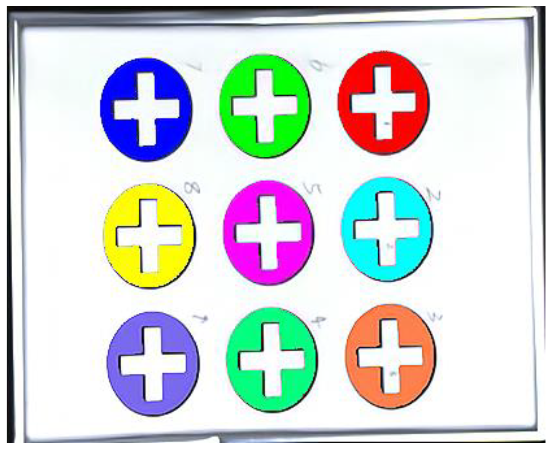
Processes 13 00238 g001
Figure 2. Photo of chessboard.
Processes 13 00238 g002
Figure 3. (a) Eye-to-hand configuration; (b) Eye-in-hand configuration.
Processes 13 00238 g003
Figure 4. Camera and wheel hub placement position.
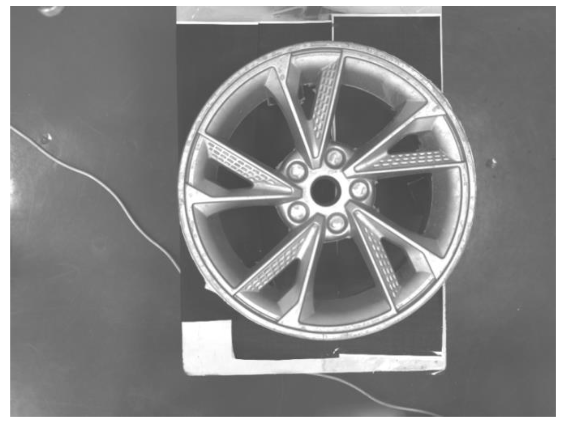
Processes 13 00238 g004
Figure 5. Image of the wheel hub casting.
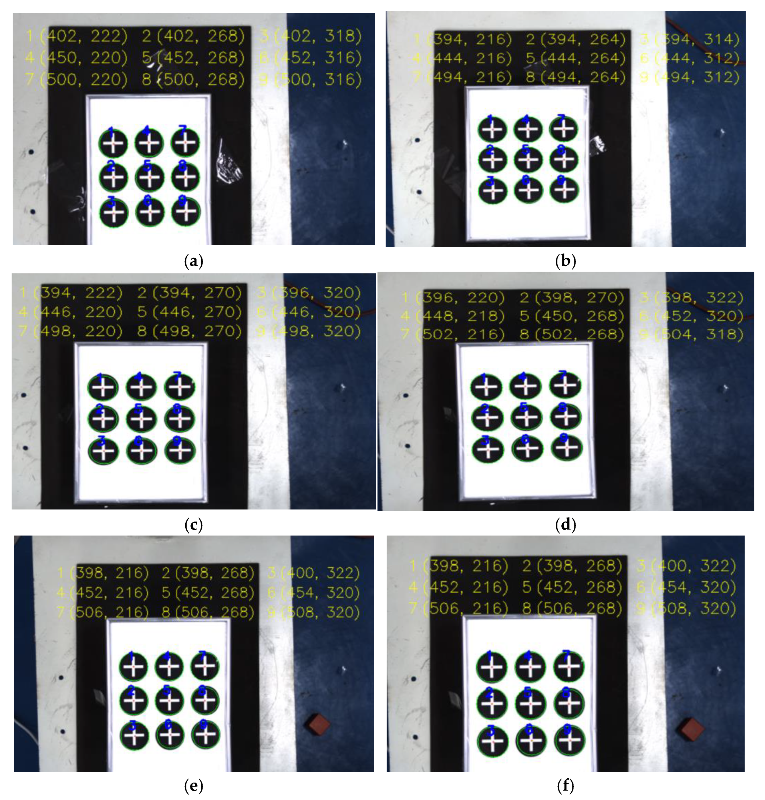
Processes 13 00238 g005
Figure 6. (a) Raw image brightness information; (b) Histogram equalization results.
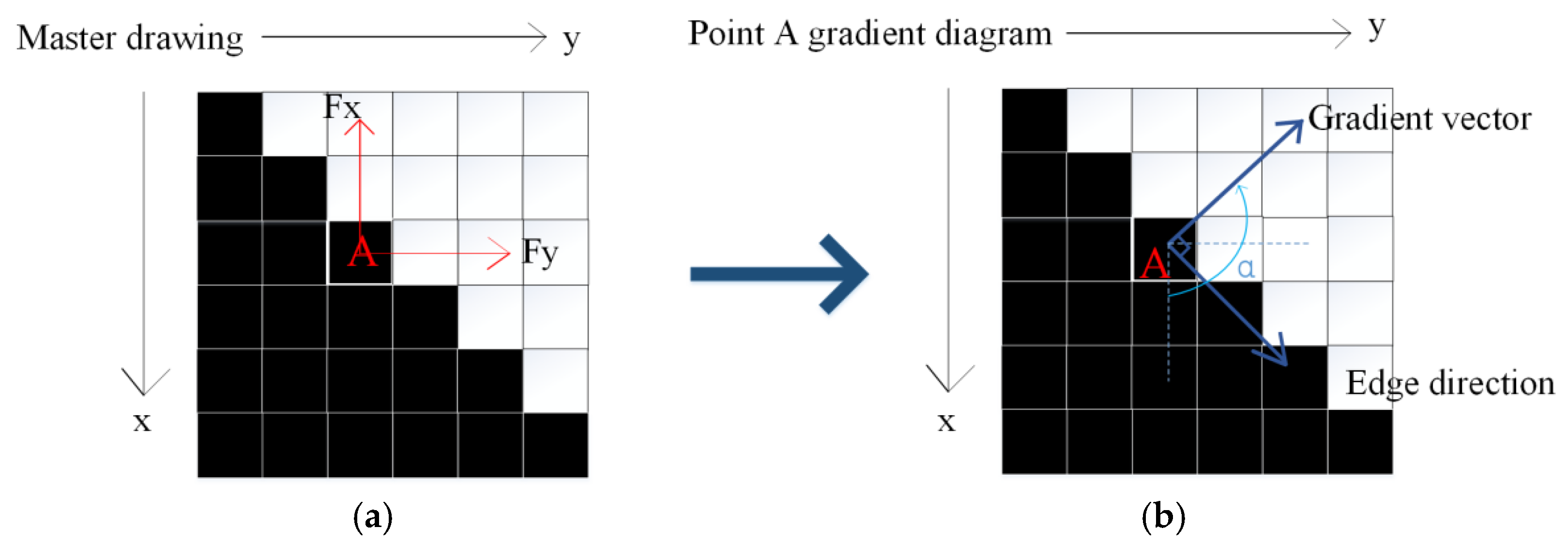
Processes 13 00238 g006
Figure 7. (a) Point A original image; (b) Point A gradient diagram.
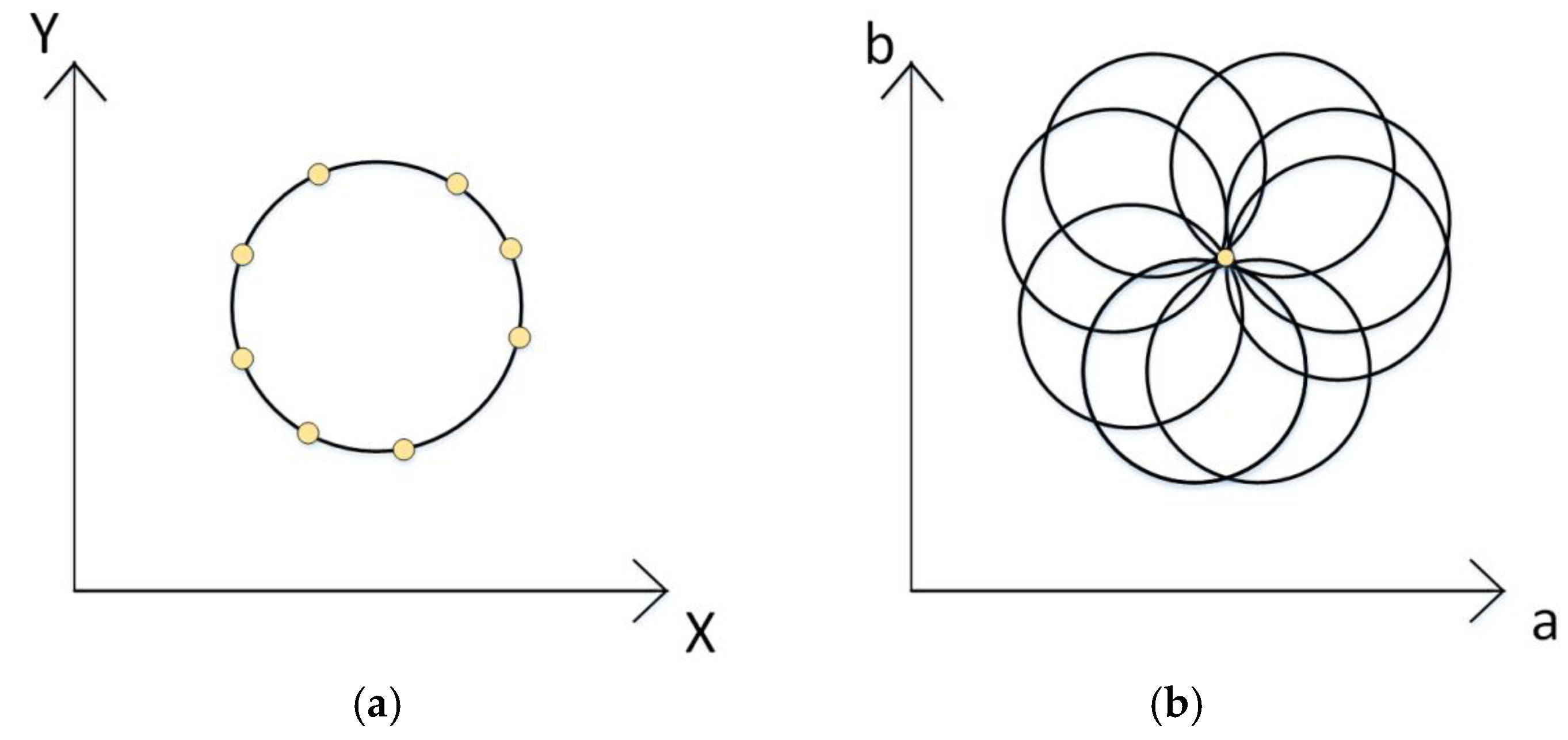
Processes 13 00238 g007
Figure 8. (a) Image space; (b) Parameter space.
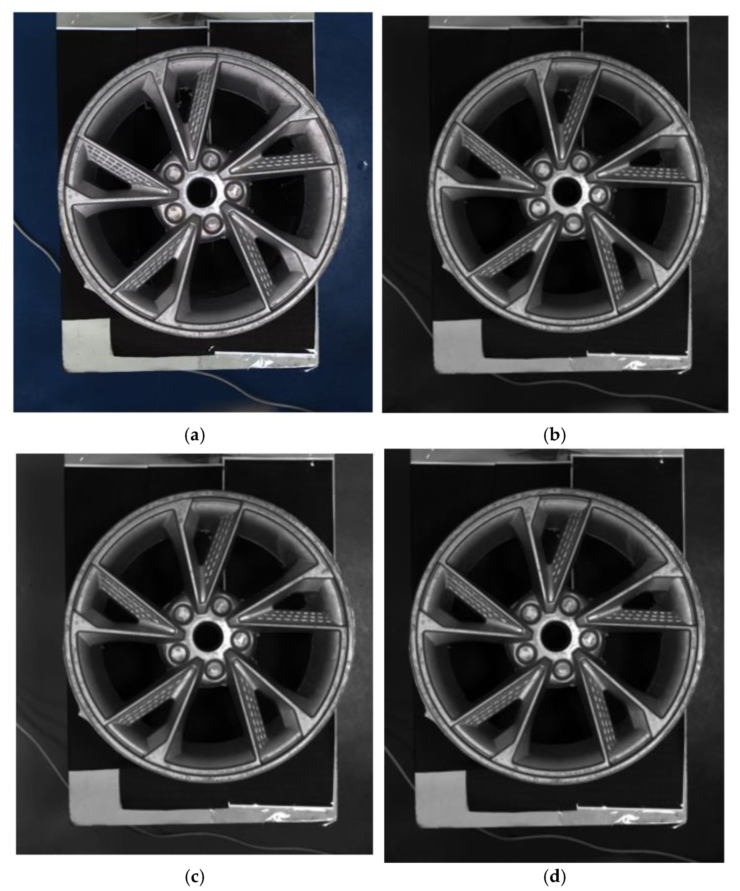
Processes 13 00238 g008
Figure 9. (a) An image with a height of 0; (b) An image with a height of 4; (c) An image with a height of 8; (d) An image with a height of 12; (e) An image with a height of 16; (f) An image with a height of 20.
Processes 13 00238 g009
Figure 10. Relationship between height and magnification.
Processes 13 00238 g010
Figure 11. Location map of the burr points on the wheel hub.
Processes 13 00238 g011
Figure 12. Schematic diagram of path angles in space.
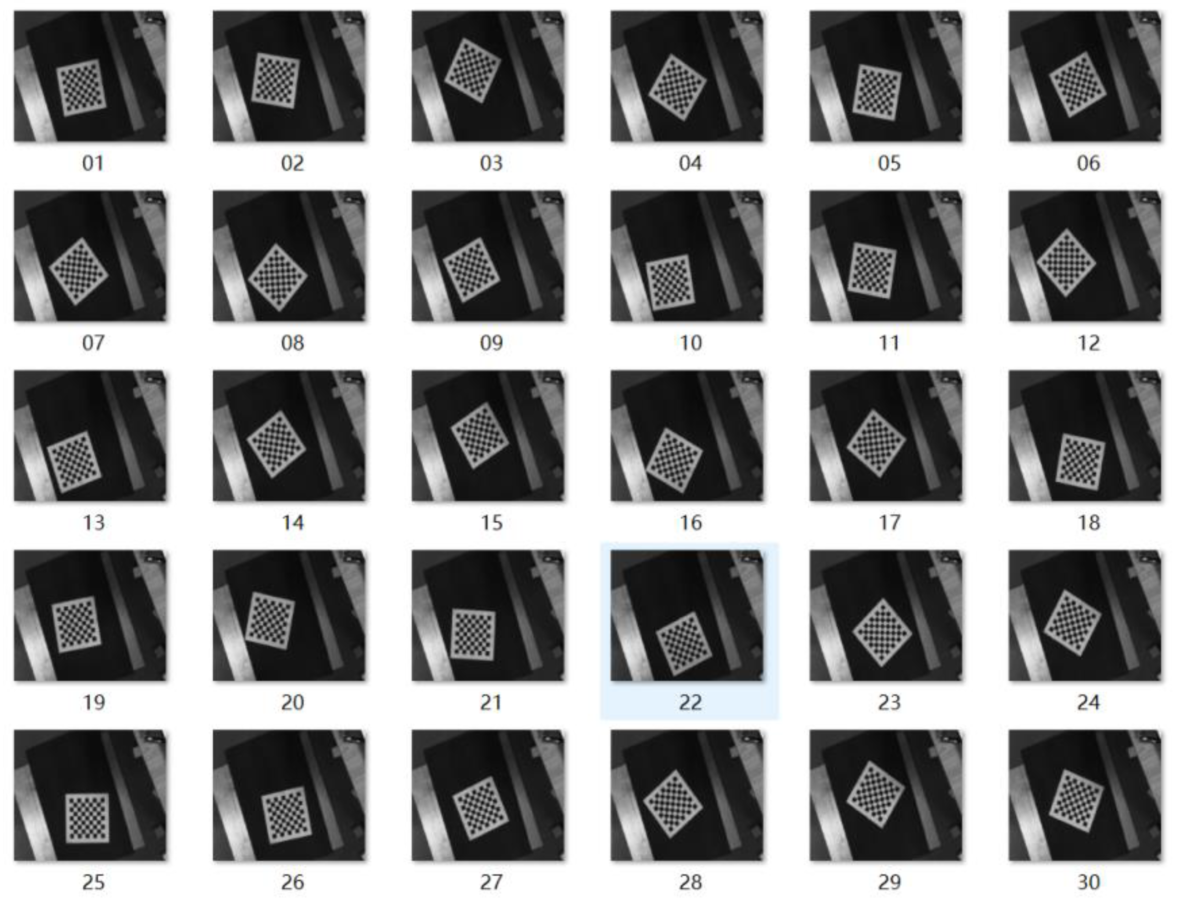
Processes 13 00238 g012
Figure 13. Images of the checkerboard in 30 different configurations.
Processes 13 00238 g013
Figure 14. Calibration plate processing diagram.
Processes 13 00238 g014
Figure 15. (a) Original image; (b) Gray mean image; (c) Gray maximum image; (d) Weighted mean image.
Processes 13 00238 g015
Figure 16. (a) Median filtering processing results; (b) Mean filtering processing results.
Processes 13 00238 g016
Figure 17. Image after HE with enhanced high-frequency regions.
Processes 13 00238 g017
Figure 18. Image combined with sobel operator processing and grayscale image.
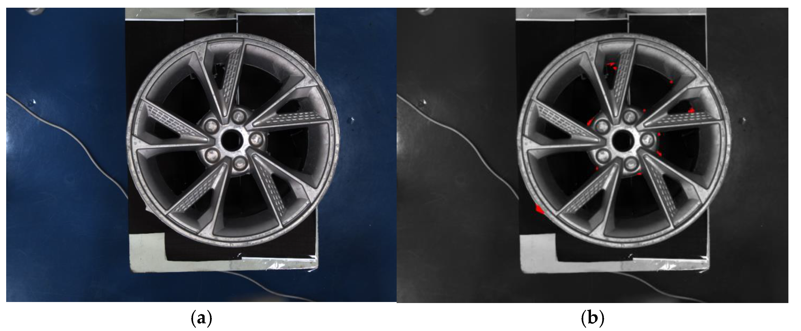
Processes 13 00238 g018
Figure 19. (a) Original image; (b) Burr extraction result.
Processes 13 00238 g019
Figure 20. Height error compensation results.
Processes 13 00238 g020
Figure 21. (a) Burr image at 0 mm height; (b) Burr image at 60 mm height.
Processes 13 00238 g021
Figure 22. Comparison of centroid coordinates with standard values before and after compensation.
Processes 13 00238 g022
Figure 23. 3D burr point information.
Processes 13 00238 g023
Figure 24. Path graph not processed by optimization algorithm.
Processes 13 00238 g024
Figure 25. Path graph processed by ACO algorithm.
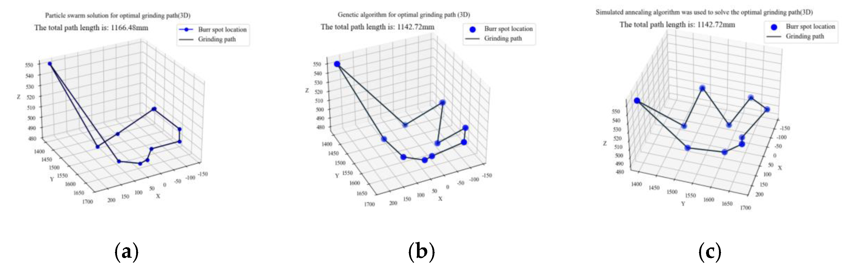
Processes 13 00238 g025
Figure 26. (a) PSO algorithms results; (b) GA algorithms results; (c) SA algorithms results.
Processes 13 00238 g026
Figure 27. The relationship between the number of iterations of four intelligent optimization algorithms and the minimum path length.
Processes 13 00238 g027
Figure 28. (a) ACO algorithms; (b) PSO algorithms; (c) GA algorithms; (d) SA algorithms.
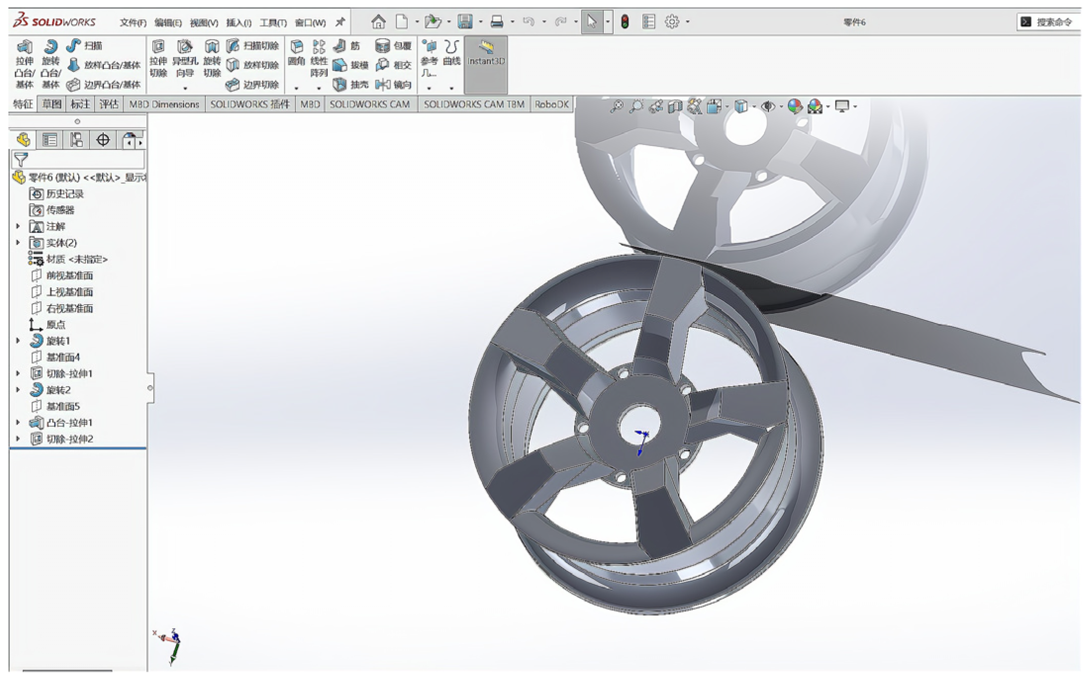
Processes 13 00238 g028aProcesses 13 00238 g028b
Figure 29. 3D model of wheel hub casting.
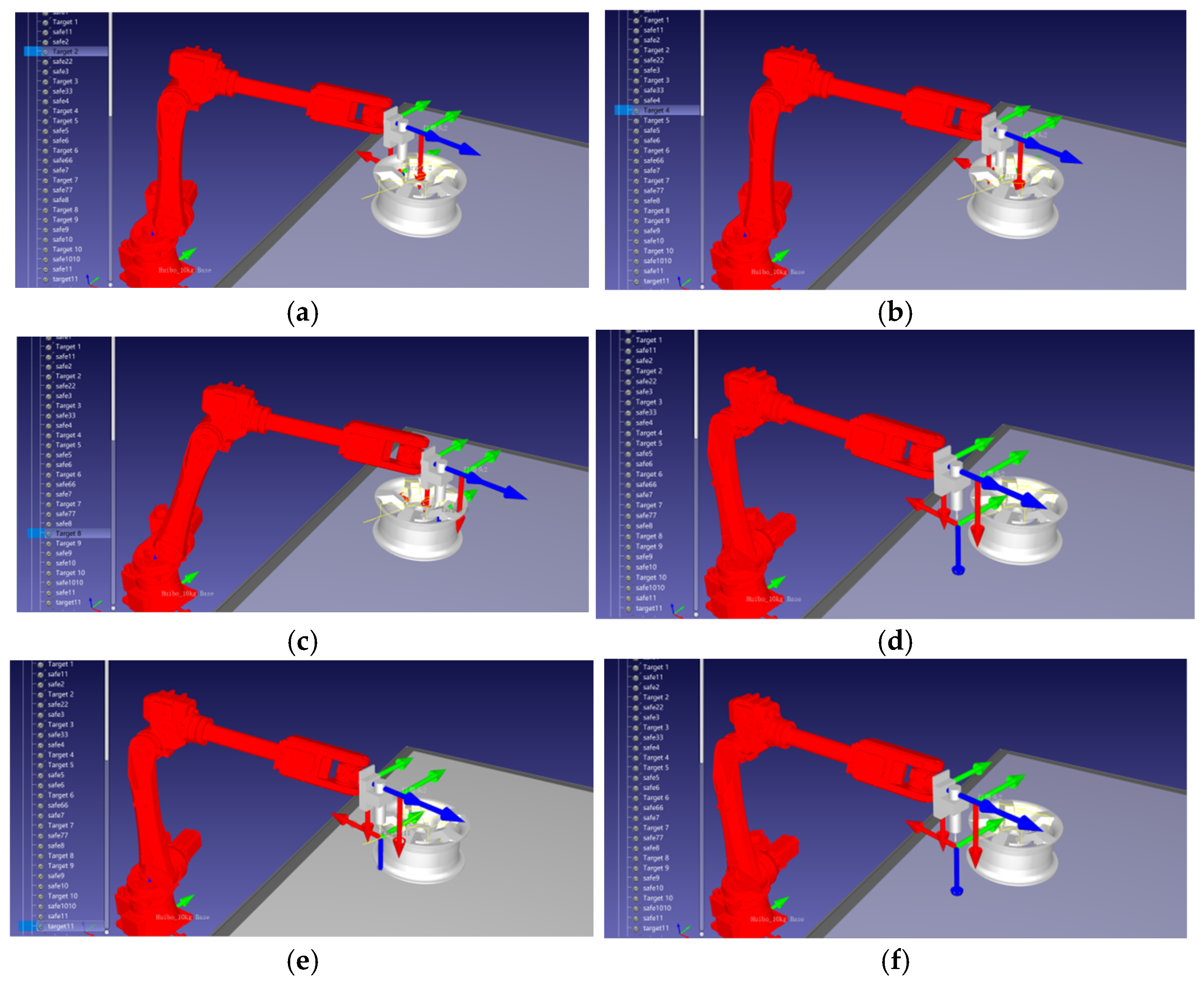
Processes 13 00238 g029
Figure 30. (a) Burr point; (b) Burr point 4; (c) Burr point 8; (d) Burr point 10; (e) Burr point 11; (f) Retract point.
Processes 13 00238 g030
Figure 31. Robot grinding wheel hub experimental platform.
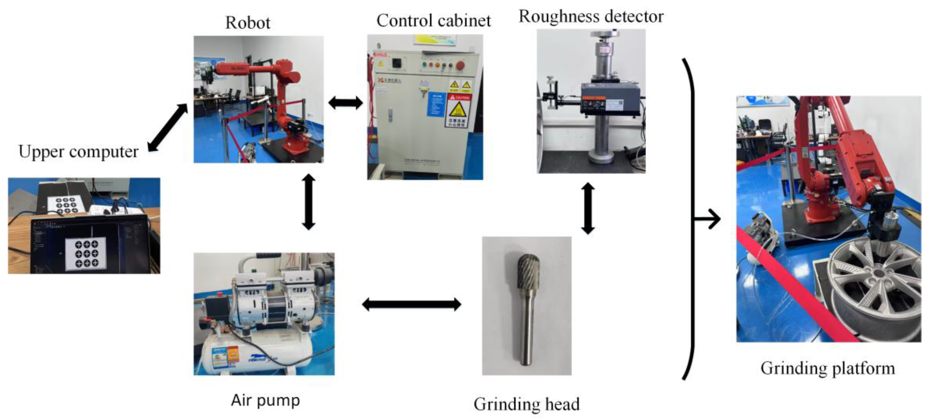
Processes 13 00238 g031
Figure 32. Composition of the robot grinding system.
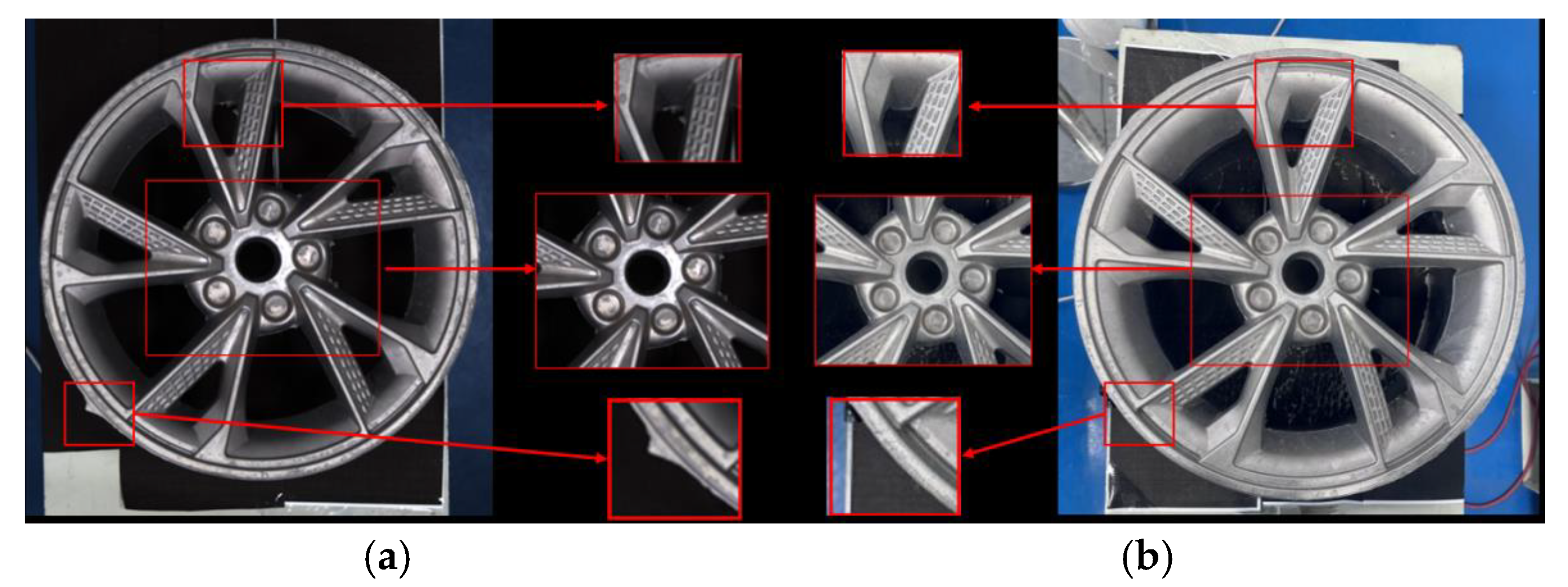
Processes 13 00238 g032
Figure 33. Burrs 7 and 8 on the wheel hub casting.
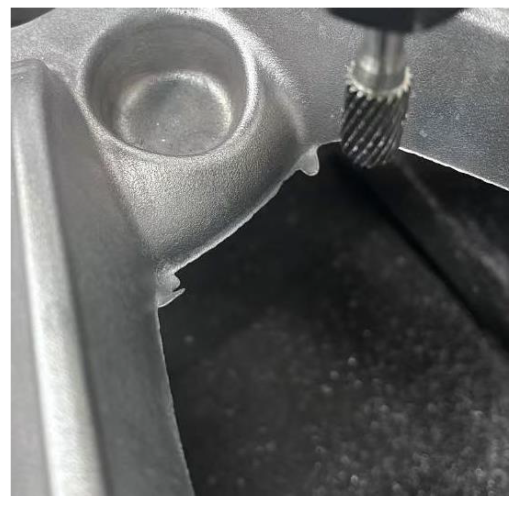
Processes 13 00238 g033
Figure 34. (a) Image at 200 rpm; (b) Image at 400 rpm; (c) Image at 600 rpm; (d) Image at 800 rpm.
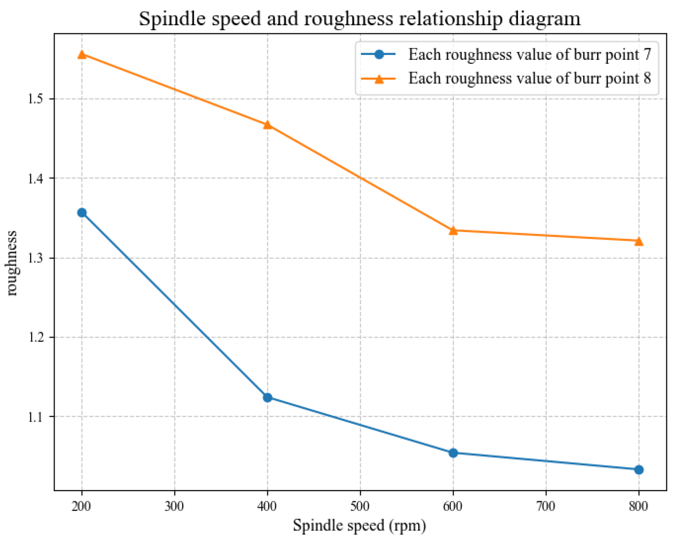
Processes 13 00238 g034
Figure 35. Relationship between spindle speed and roughness after burr grinding.
Processes 13 00238 g035
Figure 36. (a) Diagram before burr grinding; (b) Diagram of burr grinding after grinding.
Processes 13 00238 g036
Table 1. Experiment on the elevation height and circular measurement size of the calibration plate.
Elevation Height (mm)Magnification
00.00489
400.004979
800.00506
1200.00515
1600.00524
2000.00533
Table 2. Basic parameter settings for the ant colony optimization algorithm.
Parameter MeaningParameter AbbreviationValue
Number of antsants100
Maximum iterationsiterations5000
Pheromone emphasis factorα3
Minimum pheromone concentrationτmin1
Maximum pheromone concentrationτmax10
Pheromone volatility coefficientants100
Table 3. Internal parameters of the camera.
Internal Parameter f x f y u 0 v 0 s
Value8373.88362.12024.31348.20
Table 4. Camera distortion coefficients.
Parameter k 1 k 2 p 1 p 2 k 3
Value−0.05920.6125000
Table 5. Transformation matrix parameters between the camera and the robot.
Parameterabcdef
Value−0.05920.61250001346.5
Table 6. Parameters of the tool–hand coordinate t1.
NameValue (mm)NameValue (°)
X−307.378A−0.045
Y0.556B89.982
Z98.660C179.980
Table 7. Centroid coordinates position.
PositionCentroid Coordinates at 0 mm Height (X, Y)Centroid Coordinates at 60 mm Height (X, Y)Compensated Centroid Coordinates (X, Y)
1(538, 163)(550, 144)(534, 168)
2(550, 165)(559, 154)(547, 168)
3(688, 201)(704, 189)(683, 204)
4(623, 274)(635, 263)(619, 277)
5(739, 271)(756, 264)(734, 273)
6(489, 310)(495, 293)(487, 314)
7(662, 332)(673, 324)(658, 334)
8(665, 380)(674, 374)(662, 381)
9(511, 422)(513, 412)(510, 424)
10(617, 432)(623, 426)(615, 433)
11(374, 529)(366, 518)(376, 532)
Disclaimer/Publisher’s Note: The statements, opinions and data contained in all publications are solely those of the individual author(s) and contributor(s) and not of MDPI and/or the editor(s). MDPI and/or the editor(s) disclaim responsibility for any injury to people or property resulting from any ideas, methods, instructions or products referred to in the content.

