A Joint Prediction of the State of Health and Remaining Useful Life of Lithium-Ion Batteries Based on Gaussian Process Regression and Long Short-Term Memory

Abstract

To comprehensively evaluate the current and future aging states of lithium-ion batteries, namely their State of Health (SOH) and Remaining Useful Life (RUL), this paper proposes a joint prediction method based on Gaussian Process Regression (GPR) and Long Short-Term Memory (LSTM) networks. First, health features (HFs) are extracted from partial charging data. Subsequently, these features are fed into the GPR model for SOH estimation, generating SOH predictions. Finally, the estimated SOH values from the initial cycle to the prediction start point (SP) are input into the LSTM network in order to predict the future SOH trajectory, identify the End of Life (EOL), and infer the RUL. Validation on the Oxford Battery Degradation Dataset demonstrates that this method achieves high accuracy in both SOH estimation and RUL prediction. Furthermore, the proposed approach can directly utilize one or more health features without requiring dimensionality reduction or feature fusion. It also enables RUL prediction at the early stages of a battery’s lifecycle, providing an efficient and reliable solution for battery health management. However, this study is based on data from small-capacity batteries and does not yet encompass applications in large-capacity or high-temperature scenarios. Future work will focus on expanding the data scope and validating the model’s performance in real-world systems, driving its application in practical engineering scenarios.

1. Introduction

With the rapid development of electric vehicles and renewable energy storage systems, lithium-ion batteries, as key energy storage devices, have garnered significant attention for their performance and safety [1]. State of Health (SOH) and Remaining Useful Life (RUL) are two crucial parameters for evaluating battery performance [2,3]. Accurately estimating these parameters is essential for ensuring the safe and efficient operation of battery systems, as well as for reducing operational costs and preventing unexpected failures [4].

SOH is defined as the ratio of the current maximum available capacity of the battery to its rated capacity [5], expressed by the following equation:

$$\mathrm{S}\mathrm{O}\mathrm{H}={\displaystyle \frac{Q_{\mathrm{c}\mathrm{u}}}{Q_{\mathrm{e}}}}\times 100\mathrm{\%}$$

(1)

where $Q_{\mathrm{c}\mathrm{u}}$ represents the current maximum available capacity of the battery and $Q_{\mathrm{e}}$ represents the rated capacity of the battery.

When the current maximum available capacity of the battery drops to 80% of its rated capacity, i.e., a SOH of ≤ 80%, the battery reaches its End of Life (EOL), at which point it needs to be replaced. RUL is defined as the expected number of cycles remaining before the battery reaches its EOL, starting from its current state [6], expressed as follows:

$$\mathrm{R}\mathrm{U}\mathrm{L}={cycle}_{EOF}-{cycle}_{cu}$$

(2)

where ${cycle}_{EOF}$ represents the number of cycles at which the battery reaches its EOL; ${cycle}_{cu}$ represents the current cycle count of the battery.

Currently, SOH estimation methods can be categorized into two types: model-based methods and data-driven methods. Model-based methods estimate the SOH by constructing equivalent circuit models for the battery. For example, Schwunk et al. [7] proposed an SOH estimation method based on the PF; Bustos et al. [8] developed an approach using the DF; Ranga et al. [9] introduced a method based on the UKF; Rahimifard et al. [10] proposed an ASVSF-VBL; Fahmy et al. [11] presented a DAUKF-CCA; and Yang et al. [12] also implemented an SOH estimation approach using the UKF. However, due to the complexity of the internal battery environment and the uncertainty of external operating conditions, developing an accurate model remains a significant challenge [13].

In contrast, data-driven methods avoid the complexity of the modeling process by analyzing the historical operating data of batteries and utilizing deep learning or machine learning techniques to estimate the SOH. As a result, these methods have gained significant attention and recognition in recent years [14]. For example, Alberto et al. [15] proposed an SOH estimation method based on an FC-FNN; Rahimian et al. [16] introduced a method using an NN; Safavi et al. [17] developed an approach combining a CNN-LSTM; Lee et al. [18] presented a method utilizing an MNN-LSTM; and Teixeira et al. [19] proposed a GRU-based SOH estimation method.

In data-driven SOH estimation, the selection of health features (HFs) plays a critical role. Jia et al. [20] extracted HFs from the discharge process and used GPR for SOH estimation. However, in practical applications, the discharge conditions of batteries are often difficult to measure accurately, making data collection challenging. In comparison, data collection during the charging process is more convenient. Feng et al. [21] used features such as constant-current and constant-voltage charging times as HFs and employed IGPR for SOH estimation. Similarly, Dai et al. [22] extracted HFs such as constant-current and constant-voltage charging times from the complete charging process and utilized DA-BiLSTM networks for SOH estimation. Liu [23] further considered that batteries are not always charged from zero during the charging process and extracted the constant-current charging time from a state of charge (SOC) of 20% to the end of charging as an HF, using GPR for SOH estimation. However, this method overlooks scenarios where the battery might not be fully charged.

RUL prediction is primarily based on data-driven methods. For instance, Chang et al. [24] used the first 50% or 70% of a battery’s data to train an LSTM model and tested it with the remaining data to predict the RUL. Liu et al. [25] employed the first 50% or 60% of a battery’s data to train a CEEMDAN-PSO-BiGRU model and tested it with the remaining data for RUL prediction. Similarly, Zou et al. [26] utilized the first 40% or 50% of a battery’s data to train a CEEMDAN-PSO-BiGRU model, testing it with the remaining data for RUL prediction. Tang et al. [27] adopted the first 50% of a battery’s data to train a CEEMDAN-IGWO-BiGRU model and tested it with the remaining data for RUL prediction. These RUL prediction methods typically focus on a single battery, using its early-stage data for model training and later-stage data for testing. Since only a portion of the historical data is used, the model is unable to fully learn the complete degradation cycle of the battery, resulting in certain limitations [28]. Furthermore, such methods cannot provide RUL predictions during the early stages of battery usage, which poses constraints in practical applications.

SOH and RUL are both parameters that reflect battery aging, with the SOH representing the current aging state and the RUL indicating future aging trends. To comprehensively estimate the battery’s aging status, it is essential to jointly predict both the SOH and RUL. For example, Li et al. [29] proposed a joint SOH and RUL prediction method based on GPR-LSSVM; Dong et al. [30] developed a method using HKFRVM; and Wang et al. [31] proposed another approach based on GPR-LSSVM for joint SOH and RUL prediction. In these methods, researchers typically extract multiple health features from battery data for SOH estimation and then use dimensionality reduction techniques to fuse these features into a single indirect health feature (IHF), which is used as the input for the SOH estimation model. During the RUL prediction process, these methods rely on predicting IHF values based on cycle numbers and subsequently inferring the SOH and RUL from the predicted IHF. This approach requires minimizing the number of health features, often using only a single composite feature, to simplify the relationship between cycle numbers and features.

Based on this, this paper proposes a joint SOH and RUL prediction method utilizing partial charging data. First, Gaussian Process Regression (GPR) is employed for SOH estimation, followed by Long Short-Term Memory (LSTM) networks for RUL prediction. The proposed method offers the following advantages:

• It leverages partial charging data, reducing dependence on complete charging data and making the model more suitable for real-world scenarios with incomplete data.
• The method imposes no restriction on the number of input features, allowing for the flexible selection of health features.
• It enables RUL prediction during the early stages of battery usage, providing earlier warning capabilities to help extend battery lifespan and prevent unexpected failures.

The remainder of this paper is organized as follows: Section 2 introduces the theoretical foundations, dataset, correlation analysis, model architecture, and evaluation metrics. Section 3 presents the model validation, result analysis, and a discussion. Section 4 summarizes the work of this study.

2. Theoretical Foundation

2.1. GPR

GPR [32] is a non-parametric Bayesian regression method that models data by assuming a certain relationship between data points. GPR excels in handling small sample datasets and providing uncertainty estimates for predictions, making it highly adaptable. The mathematical foundations of GPR are detailed below.

• Definition of Gaussian Process

A Gaussian process is a stochastic process defined over a function space. Its core idea is to assume that the function values $f\left(x\right)$ follow a Gaussian distribution. For any set of inputs $x=\left\{x_1,x_2,\dots ,x_n\right\},$ their corresponding function values $f=\left\{f\right(x_1),f(x_2),\dots ,f(x_n\left)\right\}$ follow a multivariate Gaussian distribution.

A Gaussian process can be denoted as follows:

$$f\sim GP\left(m\left(x\right),K\left(x,x^{\prime }\right)\right)$$

(3)

where $m\left(x\right)$ is the mean function, representing the expected value of the function at input point x; $K\left(x,x^{\prime }\right)$ is the covariance function (or kernel function), which describes the correlation between two input points. The covariance function is typically chosen to be a symmetric positive definite kernel.

In practical applications, the mean function is often assumed to be $m\left(x\right)=0$, leaving only the definition of the covariance function $K\left(x,x^{\prime }\right)$ to be specified.

2.

Covariance Function and Expectation

The mean function $m\left(x\right)$ and the covariance function $K\left(x,x^{\prime }\right)$ are defined as follows:

$$m\left(x\right)=E\left[f\left(x\right)\right]$$

(4)

$$K\left(x,x^{\prime }\right)=E\left[\left(f\left(x\right)-m\left(x\right)\right)-\left(f\left(x^{\prime }\right)-m\left(x^{\prime }\right)\right)\right]$$

(5)

where $E\left[f\left(x\right)\right]$ represents the expected value of $f\left(x\right)$, while $K\left(x,x^{\prime }\right)$ represents the covariance between $f\left(x\right)$ and $f\left(x^{\prime }\right)$, reflecting the correlation between these two input points.

3.

Observation Data Model

Consider a set of observation data $\left\{\right(x_i,y_i){\}}_{i=1}^n$, where $x_i$ represents the input and $y_i$ represents the observed value. It is assumed that the observed value is composed of the true function value $f\left(x_i\right)$ and independent and identically distributed Gaussian noise ${ϵ}_i$, as follows:

$$y_i=f\left(x_i\right)+{ϵ}_i,{ϵ}_i\sim N\left(0,{\sigma }_n^2\right)$$

(6)

These observations can be expressed as follows:

$$y=f\left(X\right)+ϵ$$

(7)

where $y=[y_1,y_2,\dots ,y_n{]}^{\mathrm{\top }},f\left(X\right)=[f\left(x_1\right),f\left(x_2\right),\dots ,f\left(x_n\right){]}^{\mathrm{\top }}$, and the noise term $ϵ$ follows a Gaussian distribution with a mean of zero and variance ${\sigma }_n^2$, denoted as $ϵ\sim N(0,{\sigma }_n^{2}I)$.

4.

Joint Gaussian Distribution

Since $f\left(X\right)$ follows a Gaussian process $GP(0,K)$, the observed values $y$ follow a joint Gaussian distribution:

$$y\sim N\left(0,K\left(X,X\right)+{\sigma }_n^{2}I\right)$$

(8)

5.

Prediction for a New Input Point

For a new input $x^{*}$, the distribution of its corresponding output $f\left(x^{*}\right)$ can be predicted. According to the properties of Gaussian processes, the joint distribution can be expressed as follows:

$$\left[\begin{array}{c}y\\ f\left(x^{*}\right)\end{array}\right]\sim N\left(0,\left[\begin{array}{cc}K\left(X,X\right)+{\sigma }_n^{2}I& K\left(X,x^{*}\right)\\ K\left(x^{*},X\right)& K\left(x^{*},x^{*}\right)\end{array}\right]\right)$$

(9)

where $K\left(X,x^{*}\right)$ is the covariance vector between the training points and the test point $x^{*}$, and $K\left(x^{*},x^{*}\right)$ is the covariance of the test point with itself.

Using the properties of conditional Gaussian distributions, the predictive distribution of $f\left(x^{*}\right)$ given $X$, $y$, and $x^{*}$ follows a Gaussian distribution:

$$f\left(x^{*}\right)\mid X,y,x^{*}\sim N\left(\mu \left(x^{*}\right),{\sigma }^2\left(x^{*}\right)\right)$$

(10)

where the mean and variance are given by the following equations:

$$\mu \left(x^{*}\right)=K\left(x^{*},X\right)[K\left(X,X\right)+{\sigma }_n^{2}I{]}^{-1}y$$

(11)

$${\sigma }^2\left(x^{*}\right)=K\left(x^{*},x^{*}\right)-K\left(x^{*},X\right)[K\left(X,X\right)+{\sigma }_n^{2}I{]}^{-1}K\left(X,x^{*}\right)$$

(12)

6.

Hyperparameter Optimization and Kernel Function Selection

In practical applications, the kernel function $K\left(x,x^{\prime }\right)$ and its hyperparameters are critical to the performance of GPR. Commonly used kernel functions include the Radial Basis Function (RBF) kernel, the Matern kernel, and the linear kernel, among others. The selection of hyperparameters is typically achieved by maximizing the marginal likelihood, which is expressed as follows:

$$\mathit{log}p\left(y∣X\right)=-{\displaystyle \frac{1}{2}}{y}^{\top }[K\left(X,X\right)+{\sigma }_n^{2}I{]}^{-1}y-{\displaystyle \frac{1}{2}}log\mid K\left(X,X\right)+{\sigma }_n^{2}I\mid -{\displaystyle \frac{n}{2}}\mathit{log}2\pi$$

(13)

By optimizing this marginal likelihood function, the optimal hyperparameter settings can be obtained, thereby improving the regression performance of GPR.

2.2. LSTM

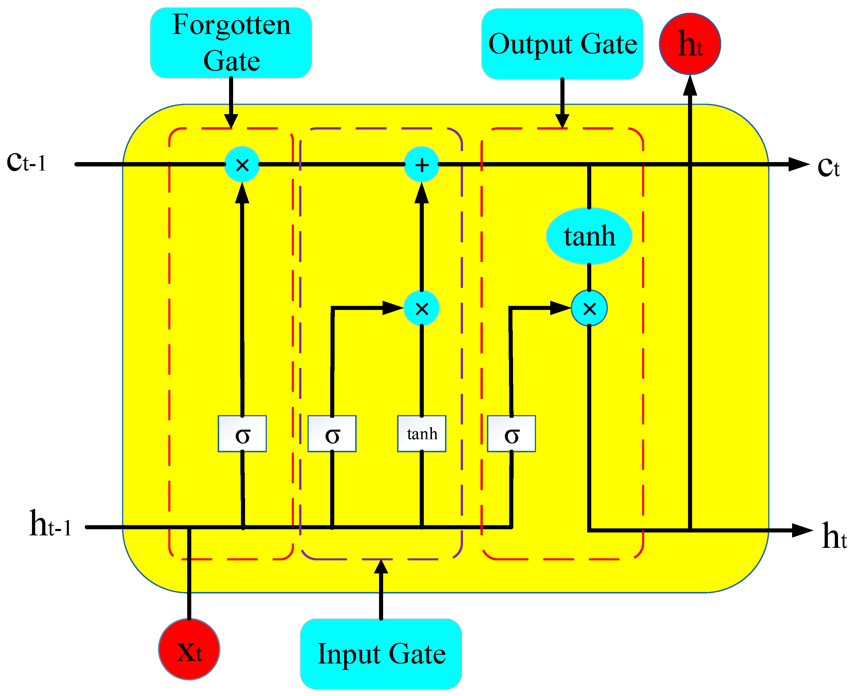
LSTM [33] is a specialized type of Recurrent Neural Network (RNN) that excels at capturing long-term dependencies in sequential data. Traditional RNNs often face challenges such as gradient vanishing or exploding when processing long time series. LSTM effectively mitigates these issues through its unique gating mechanisms.

The core of LSTM consists of three gates: the forget gate, the input gate, and the output gate, as shown in Figure 1. These gating mechanisms are responsible for selectively forgetting, updating, and outputting state information, enabling precise control over sequence information. Through these gates, LSTM can selectively retain or discard past information, making it highly effective for modeling time series data.

• Forget Gate

The forget gate controls whether information from the previous time step is passed to the next time step. Its calculation formula is as follows:

$$f_t=\sigma (w_f\times h_{\left(t-1\right)}+w_f\times x_t+b_f)$$

(14)

where $f_t$ is the output of the forget gate, representing the proportion of information to be forgotten at the current time step. $w_f$ is the weight matrix of the forget gate, which determines the influence of the previous hidden state and the current input on the forget gate. $h_{\left(t-1\right)}$ is the hidden state from the previous time step, which contains all information from the sequence up to the current time step. $x_t$ is the input data at the current time step. $b_f$ is the bias term of the forget gate. $\sigma$ is the sigmoid activation function, with an output range between 0 and 1, determining the degree of forgetting.

2.

Input Gate

The input gate controls the updating of new information at the current time step. It consists of two parts:

Input Gate Activation:

$$i_t=\sigma (w_i\times h_{\left(t-1\right)}+w_i\times x_t+b_i)$$

(15)

where $i_t$ is the output of the input gate, indicating whether new information is accepted. $w_i$ is the weight matrix of the input gate. $b_i$ is the bias term of the input gate.

Candidate values:

$$C_t=tanh\left(w_c\times h_{\left(t-1\right)}+w_c\times x_t+b_c\right)$$

(16)

where $C_t$ is the candidate value at the current time step, representing new information that can be added to the cell state. $w_c$ is the weight matrix for the candidate values. $b_c$ is the bias term for the candidate values. tanh is the hyperbolic tangent activation function, ensuring the candidate values range between −1 and 1.

3.

Cell State

The core of LSTM is the cell state $c_t$, which is responsible for carrying long-term dependency information. The update formula for the cell state is as follows:

$$c_t=f_t\times c_{\left(t-1\right)}+i_t\times C_t$$

(17)

where $c_t$ is the cell state at the current time step, containing information for long-term memory. $c_{\left(t-1\right)}$ is the cell state from the previous time step. $i_t\times C_t$ represents the update to the cell state by the input gate, determining the new information to be added to the state at the current time step.

4.

Output Gate

The output gate controls the final hidden state output. Its calculation formula is as follows:

$$o_t=\sigma (w_o\times h_{\left(t-1\right)}+w_o\times x_t+b_o)$$

(18)

where $o_t$ is the output of the output gate, determining the hidden state at the current time step. $w_o$ is the weight matrix of the output gate. $b_o$ is the bias term of the output gate.

5.

Hidden State

The final hidden state $h_t$ of the LSTM is calculated through the combination of the output gate and the cell state:

$$h_t=o_t\times \tanh \left(C_t\right)$$

(19)

where $h_t$ is the hidden state at the current time step, containing key information from the current and previous time steps. $\tanh \left(C_t\right)$ is the activation of the current cell state, with an output range between −1 and 1.

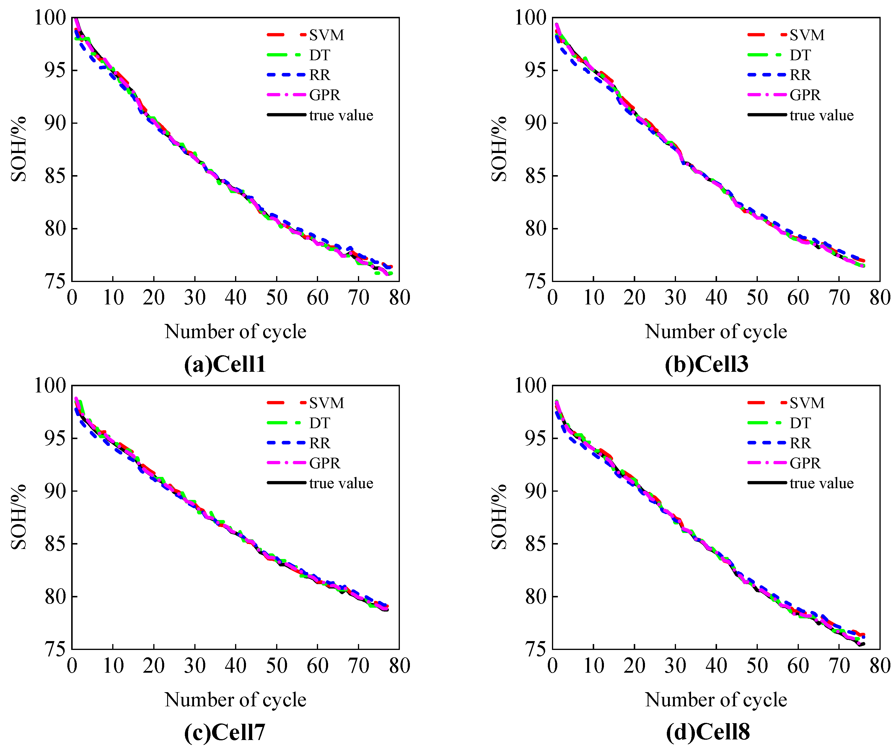
2.3. Dataset Description and Health Feature Extraction

This study uses the Oxford Battery Degradation Dataset as the source of experimental data, selecting four battery cells (Cell1, Cell3, Cell7, and Cell8) for testing. These batteries have a rated capacity of 0.74 Ah and were subjected to aging tests at a constant temperature of 40 °C. After every 100 cycles, a 1C constant current charge–discharge calibration was performed to simulate the aging behavior of the batteries during actual use.

Figure 2 illustrates the voltage curves of the battery at different cycles, using Cell1 as an example. As shown in the figure, as the number of battery cycles increases, both the charging and discharging times gradually shorten, which is visually represented by the voltage curves shifting to the left. This phenomenon indicates that the battery’s SOH degradation trend is consistent with the reduction in charging and discharging times.

In practice, it is challenging to measure battery discharge information. In contrast, collecting information during the charging process is more convenient. Therefore, this study extracts health features (HFs) from the charging process. However, the charging process may not always start from a state of charge (SOC) of 0%, nor necessarily end at full charge. Ultimately, this study uses partial charging data to extract the following HFs:

(1)

HF1: The constant current charging time in a SOC range of 20% to 80%.

(2)

HF2: The integral of the voltage curve with respect to time within a SOC range of 20% to 80%.

By extracting HFs from partial charging data, the dependence on data completeness is reduced, thereby enhancing the applicability of the proposed method.

Figure 3 illustrates the normalized degradation trends of the SOH, HF1, and HF2 with the number of cycles, using Cell1 as an example. The results show that both HF1 and HF2 exhibit clear degradation trends as the cycle count increases. These trends are highly consistent with the degradation of the SOH, indicating that the extracted HFs effectively reflect the battery’s aging state.

2.4. Correlation Analysis

To evaluate the correlation between HF1, HF2, and the SOH, this paper employs the Pearson correlation coefficient and the Spearman correlation coefficient for correlation analysis.

The Pearson correlation coefficient is defined as follows:

$$Pearson={\displaystyle \frac{E\left(XY\right)-E\left(X\right)E\left(Y\right)}{\sqrt{E\left(X^2\right)-E^2\left(X\right)}\sqrt{E\left(Y^2\right)-E^2\left(Y\right)}}}$$

(20)

where X denotes the HF and Y denotes the SOH.

The Spearman correlation coefficient is defined as follows:

$$Spearman={\displaystyle \frac{\sum _{i=1}^n\left(X_i-\overline{X}\right)\left(Y_i-\overline{Y}\right)}{\sqrt{\sum _{i=1}^n{\left(X_i-\overline{X}\right)}^2}\sqrt{\sum _{i=1}^n{\left(Y_i-\overline{Y}\right)}^2}}}$$

(21)

where $\overline{X}$ represents the average value of the HF; $\overline{Y}$ indicates the average SOH value; and n refers to the total number of samples.

Table 1. Correlation coefficient analysis.

Battery	HF1		HF2
	Pearson	Spearman	Pearson	Spearman
Cell1	99.9934	99.9956	99.9913	99.9949
Cell3	99.9950	99.9959	99.9936	99.9945
Cell7	99.9994	99.9954	99.9987	99.9921
Cell8	99.9982	99.9979	99.9975	99.9973

summarizes the Pearson and Spearman correlation coefficients between HF1 and HF2 with the SOH for the four batteries (Cell1, Cell3, Cell7, and Cell8). The results show that all correlation coefficients exceed 99.99%, indicating an extremely high correlation between the extracted health features and the SOH. This further validates that HF1 and HF2 effectively represent the battery’s health status.

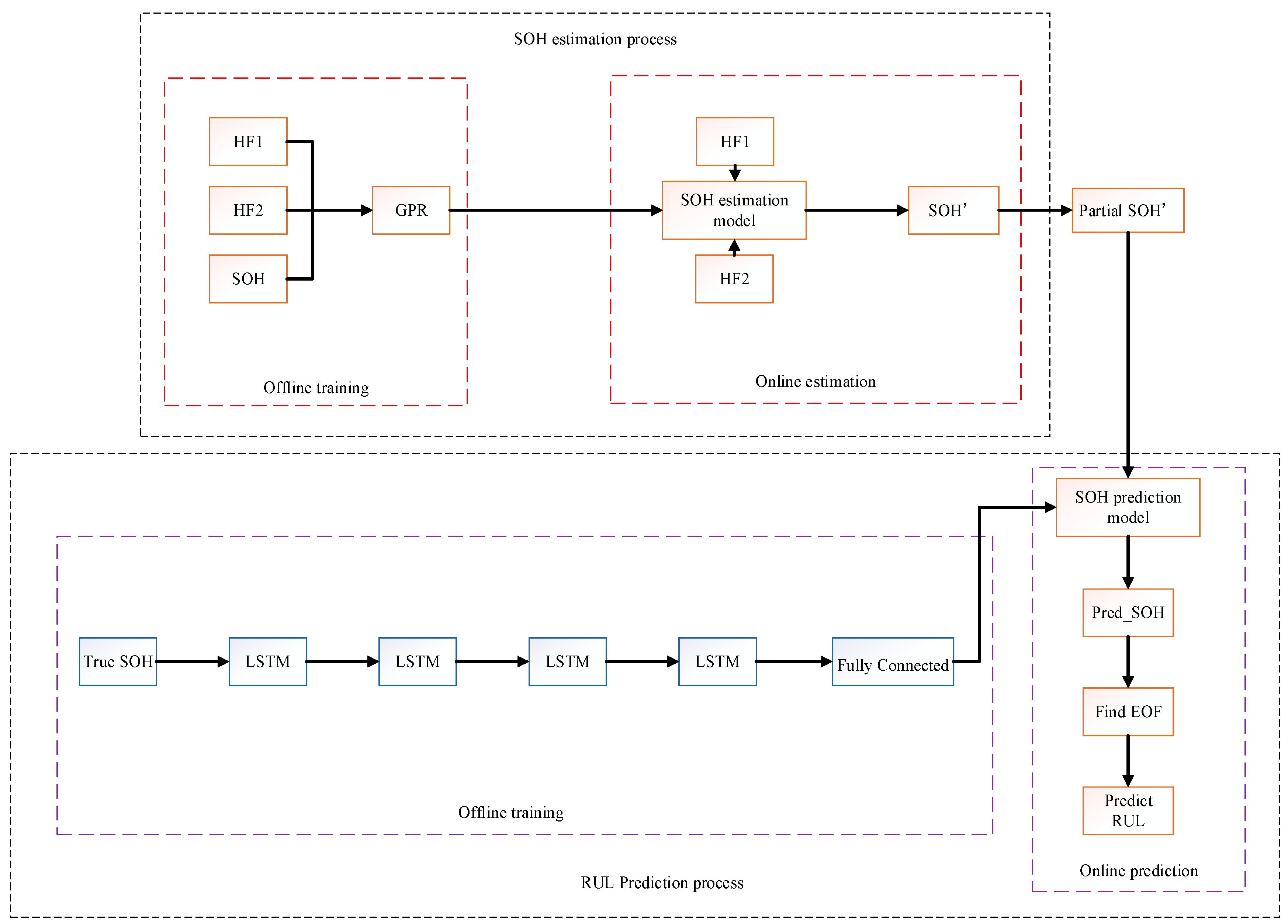
2.5. Model Structure and Parameter Settings

The structure of the proposed model is shown in Figure 4. As illustrated, the model consists of two parts: SOH estimation and RUL prediction. This structure not only enables the accurate estimation of the battery’s SOH but also facilitates the prediction of its RUL, thereby providing comprehensive state monitoring and decision support for Battery Management Systems (BMSs). All training and testing in this study were conducted in the MATLAB 2023a environment.

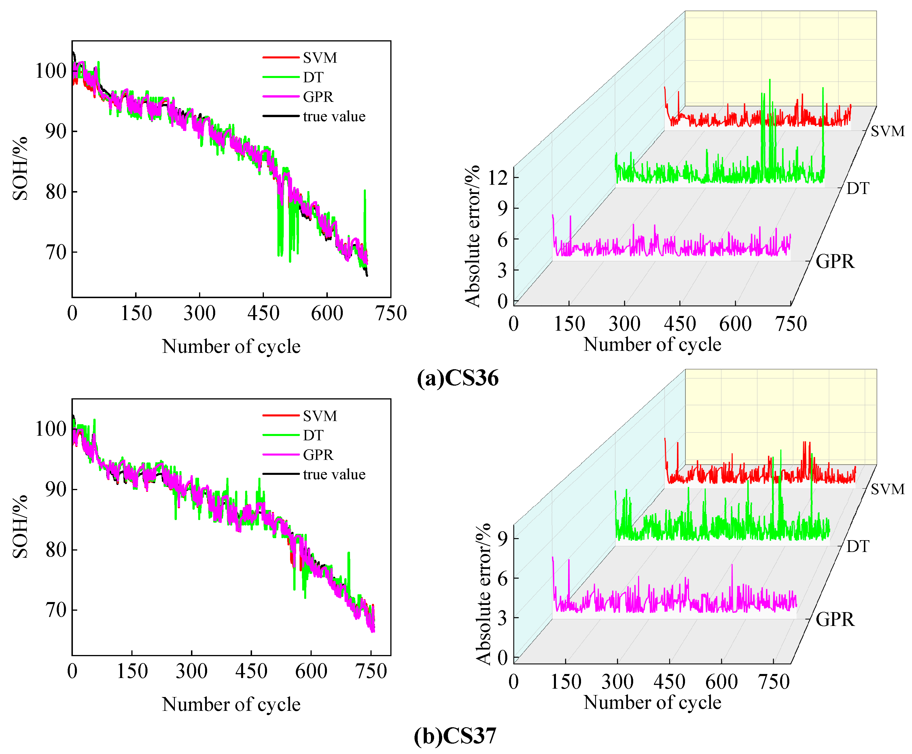
2.5.1. SOH Estimation

The SOH estimation part is divided into two phases: offline training and online testing.

• Offline Training Phase:

In this phase, HF1 and HF2 were used as input variables, and the SOH was set as the target variable to construct and train the GPR model. The constructed GPR model adopted a squared exponential kernel function, which is mathematically expressed as follows:

$$K\left(x_i,x_j\right)={\sigma }_f^2\exp \left(-{\displaystyle \frac{\parallel x_i-x_j{\parallel }^2}{2l^2}}\right)$$

(22)

where $x_i$ and $x_j$ represent the input health features, ${\sigma }_f$ is the signal amplitude, and $l$ is the length-scale hyperparameter.

To minimize the impact of differences in feature scales on model training, the input variables HF1 and HF2, and the output variable SOH were normalized to the range [0,1], using the following formula:

$$x^{\prime }={\displaystyle \frac{x-\min \left(x\right)}{\max \left(x\right)-\min \left(x\right)}}$$

(23)

where $x$ is the original feature value, $x^{\prime }$ is the normalized feature value, and $\min \left(x\right)$ and $\max \left(x\right)$ represent the minimum and maximum values of the feature, respectively.

2.

Online Testing Phase:

In this phase, HF1 and HF2 were input into the trained GPR model to obtain the estimated values of the SOH.

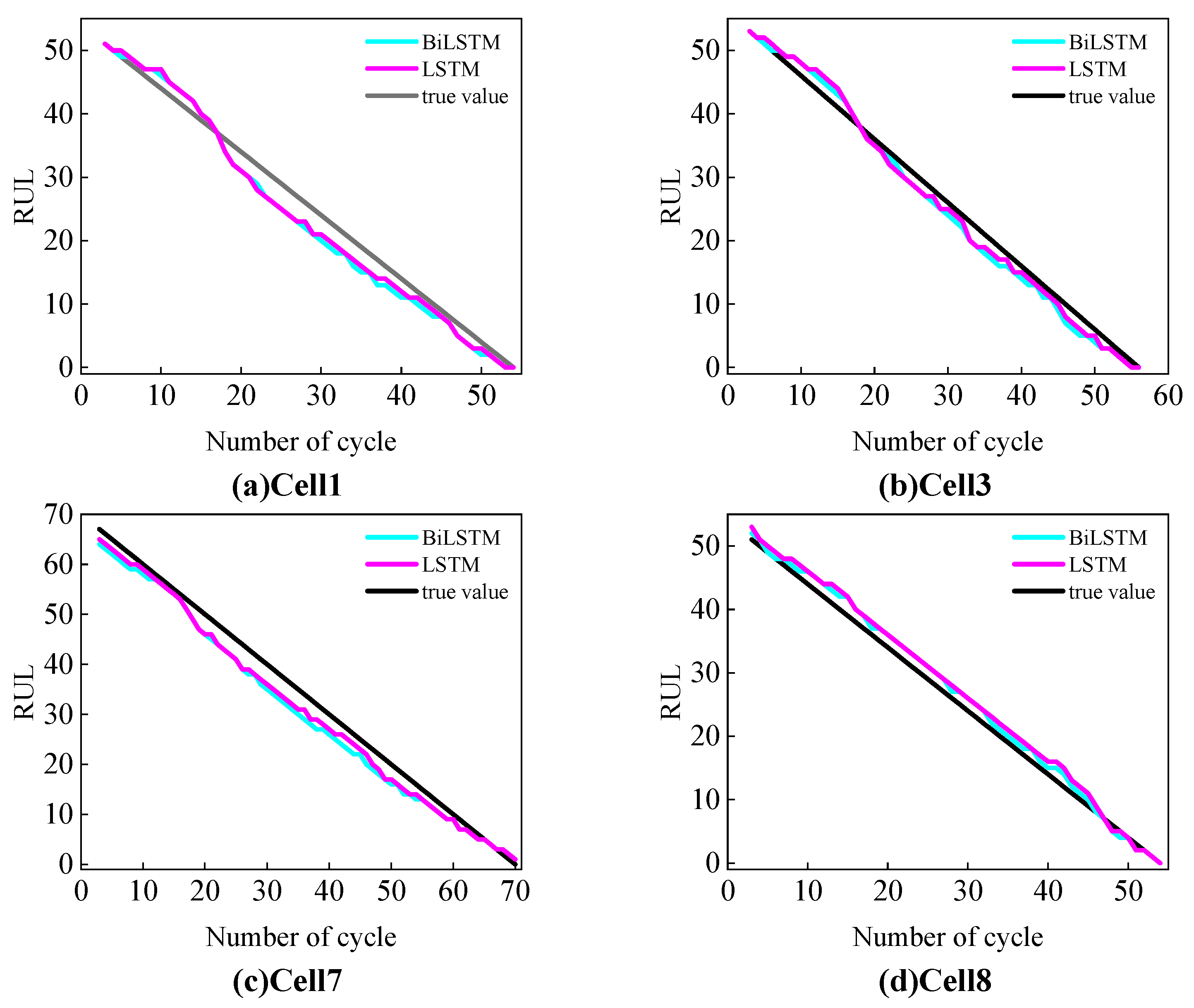
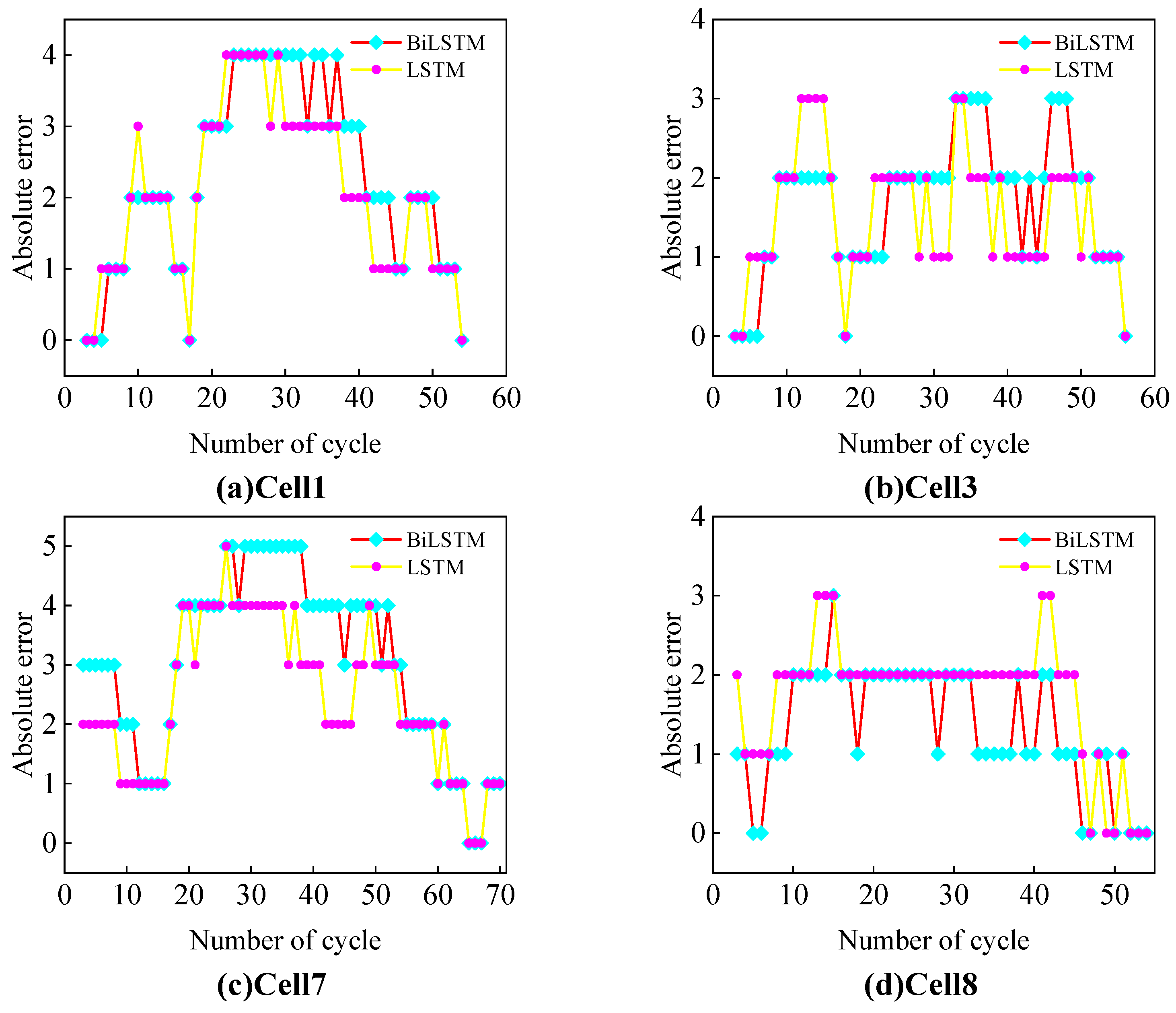
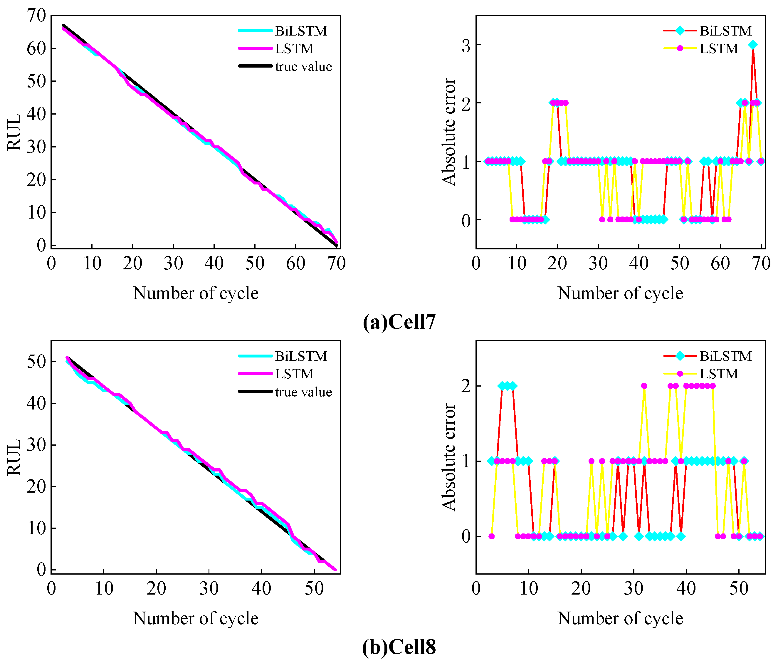
2.5.2. RUL Prediction

In the RUL prediction part, the actual SOH data were first used to train the LSTM model. The model consists of four LSTM layers and one fully connected (FC) layer. Each LSTM layer contains 20 hidden nodes, and the FC layer has one node. The initial learning rate was set to 0.001, and the Adam optimizer was used for training, the maximum number of iterations was 3000, and the sequence length was set to 2.

To enhance the training performance of the model, the SOH data were standardized. The standardized SOH data were used to generate the input and output sequences for the model. Specifically, for each input, two consecutive standardized SOH values $[{\mathrm{S}\mathrm{O}\mathrm{H}}_t,{\mathrm{S}\mathrm{O}\mathrm{H}}_{t+1}]$ were used as the input sequence, and the SOH value at the next time step, ${\mathrm{S}\mathrm{O}\mathrm{H}}_{t+2}$, was used as the output sequence.

After obtaining the SOH estimates from the GPR model, the estimates were divided into a sequence of SOH values from cycle 1 to the current SP: ${\mathrm{X}}_{\mathrm{i}\mathrm{n}\mathrm{p}\mathrm{u}\mathrm{t}}=\{\mathrm{S}\mathrm{O}{\mathrm{H}}_1,\mathrm{S}\mathrm{O}{\mathrm{H}}_2,\dots ,\mathrm{S}\mathrm{O}{\mathrm{H}}_{SP}\}$. The LSTM model was then used to predict the future SOH values. Within the predicted values, the cycle count at which SOH ≤ 80% was identified. Based on this, the RUL at the current time was calculated as follows: $\mathrm{R}\mathrm{U}\mathrm{L}={\mathrm{E}\mathrm{O}\mathrm{L}}_{\mathrm{c}\mathrm{y}\mathrm{c}\mathrm{l}\mathrm{e}}-{\mathrm{S}\mathrm{P}}_{\mathrm{c}\mathrm{y}\mathrm{c}\mathrm{l}\mathrm{e}}$.

Once the model training was completed, the SOH estimates obtained from the GPR model were divided into a sequence fragment ranging from the first cycle to just before the SP. This fragment was used as the input to the LSTM model to predict future SOH values. The cycle corresponding to the EOL was then identified from the predicted values, and the RUL at the current time was calculated accordingly.

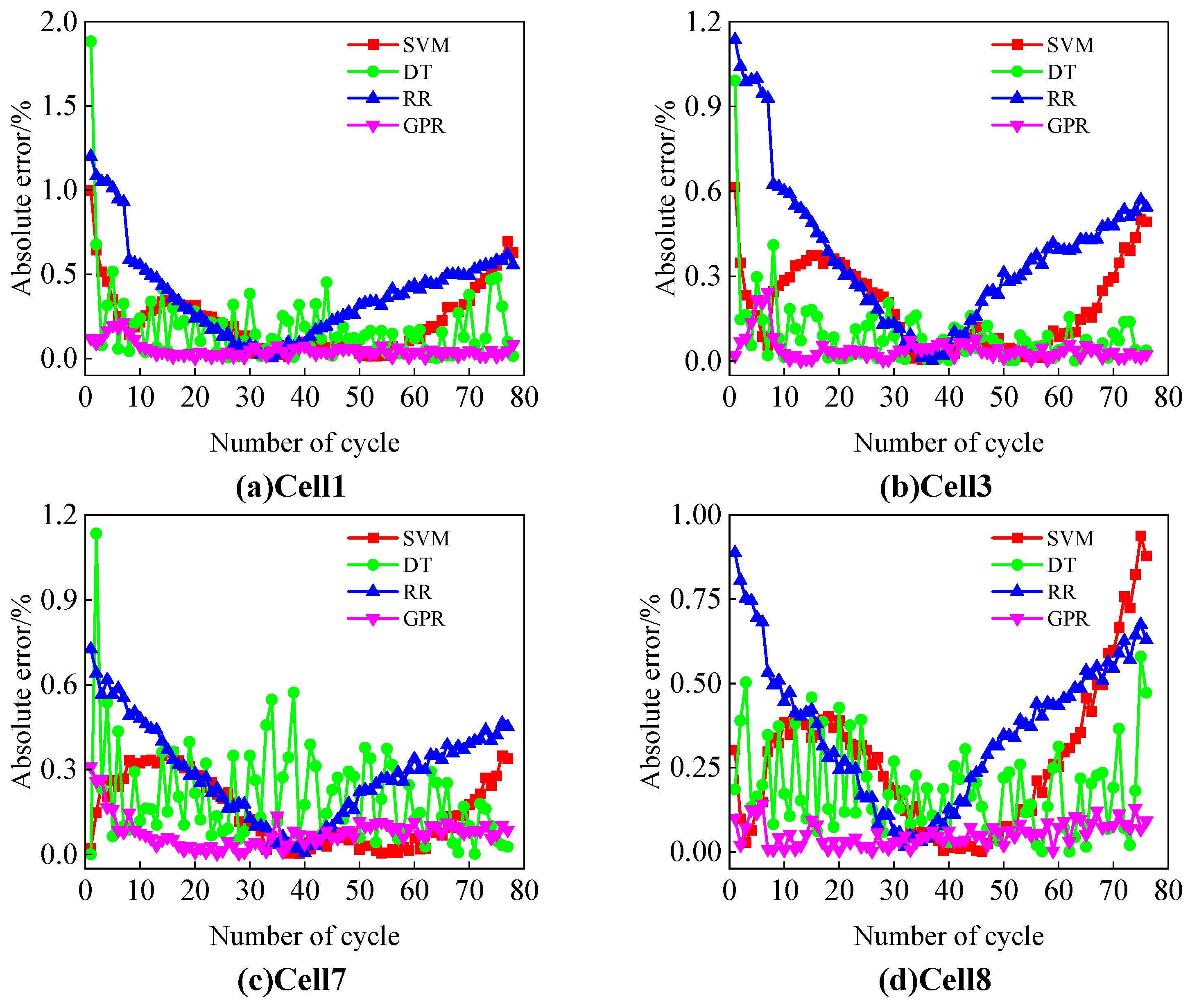
2.6. Evaluation Metrics

To evaluate the accuracy of the model’s predictions, the root mean square error (RMSE) and mean absolute error (MAE) were selected as evaluation metrics. The specific calculation methods are as follows:

$$RMSE=\sqrt{{\displaystyle \frac{1}{n}}\sum _{i=1}^n{\left({\widehat{y}}_i-y_i\right)}^2}$$

(24)

$$MAE={\displaystyle \frac{1}{n}}\sum _{i=1}^n\left|{\widehat{y}}_i-y_i\right|$$

(25)

where ${\widehat{y}}_i$ represents the predicted value for the i-th sample; $y_i$ represents the actual observed value for the i-th sample; and n denotes the number of samples.

3. Experiment and Analysis

3.1. Experiment 1

In Experiment 1, the leave-one-out method was used to validate the model, where one battery was selected as the test set while the remaining three batteries were used as the training set. This process was repeated for all batteries in the dataset. This method maximizes the utilization of the dataset and evaluates the model’s performance under different dataset combinations.

3.1.1. Analysis of SOH Estimation Results for Experiment 1

Table 2. SOH Estimation Errors under Different Models in Experiment 1.

Battery	GPR		SVM		DT		RR
	RMSE/%	MAE/%	RMSE/%	MAE/%	RMSE/%	MAE/%	RMSE/%	MAE/%
Cell1	0.0659	0.0497	0.2948	0.2229	0.3056	0.1899	0.4684	0.3837
Cell3	0.0607	0.0426	0.2402	0.1916	0.2477	0.1849	0.4615	0.3808
Cell7	0.0944	0.0768	0.1929	0.1516	0.2719	0.2093	0.3338	0.2888
Cell8	0.0632	0.0531	0.3458	0.2686	0.2276	0.1867	0.4197	0.3629

presents the results of SOH estimation. Taking Cell8 as an example, the RMSE and MAE estimated by the GPR model are 0.0632% and 0.0531%, respectively; for the SVM model, the RMSE is 0.3458% and the MAE is 0.2686%; for the Decision Tree (DT) model, the RMSE is 0.2276% and the MAE is 0.1867%; and for the Ridge Regression (RR) model, the RMSE is 0.4197% and the MAE is 0.3629%. According to the data in the table, it can be observed that the proposed GPR model achieves the highest estimation accuracy across all test sets compared to the other three models.

Figure 5 and Figure 6 further illustrate the SOH estimation results and the corresponding absolute errors for the four batteries. Combining Figure 5 and Figure 6, and Table 2, it can be observed that the GPR model exhibits lower variability in absolute error compared to the other three models, and its estimated values can better track the true values.

3.1.2. Analysis of RUL Prediction Results for Experiment 1

Table 3. RUL Prediction Errors under Different Models in Experiment 1.

Battery	LSTM		BiLSTM
	RMSE	MAE	RMSE	MAE
Cell1	2.3859	2.0769	2.6275	2.2885
Cell3	1.7105	1.5185	1.8758	1.6667
Cell7	2.7252	2.4265	3.3672	3.0147
Cell8	1.9014	1.7308	1.5254	1.3269
Average	2.1808	1.9382	2.3490	2.0742

summarizes the error results of RUL prediction for the four batteries and compares the performance of the LSTM and BiLSTM models. The results show that the LSTM model achieves an average RMSE of 2.1808 and an average MAE of 1.9382, while the BiLSTM model’s average RMSE and MAE are 2.3490 and 2.0742, respectively. The proposed LSTM model maintains low RMSE and MAE levels across all test sets and outperforms the BiLSTM model overall.

Figure 7 and Figure 8 illustrate the RUL prediction results and the corresponding absolute errors, respectively. As shown in the figures, compared to the BiLSTM model, the LSTM model exhibits smaller fluctuations in prediction error and produces prediction curves that are closer to the true values. This indicates that the LSTM model has a greater advantage in capturing the degradation trend of battery RUL.

3.2. Experiment 2

In Experiment 1, we validated the model’s performance using the leave-one-out method. To further verify the model’s robustness and wide applicability, a different experimental design was adopted in Experiment 2. In this experiment, two batteries were selected as the training set, and the other two batteries were used as the test set, allowing us to evaluate the model’s performance under different training and testing dataset combinations.

3.2.1. Analysis of SOH Estimation Results for Experiment 2

Table 4. SOH Estimation Errors under Different Models in Experiment 2.

Training Set	Test Set	GPR		SVM		DT		RR
		RMSE/%	MAE/%	RMSE/%	MAE/%	RMSE/%	MAE/%	RMSE/%	MAE/%
Cell1 and Cell3	Cell7	0.1057	0.0869	0.2409	0.2103	0.3852	0.3126	0.3182	0.2769
	Cell8	0.0670	0.0581	0.3495	0.2715	0.3430	0.2720	0.3735	0.3221
Cell1 and Cell7	Cell3	0.0607	0.0378	0.2619	0.2072	0.3994	0.3204	0.4644	0.3850
	Cell8	0.0660	0.0526	0.3309	0.2573	0.4111	0.3392	0.4372	0.3781
Cell1 and Cell8	Cell3	0.0485	0.0323	0.3285	0.2707	0.3617	0.2815	0.4221	0.3444
	Cell7	0.0878	0.0721	0.3046	0.2775	0.3999	0.3136	0.3365	0.2891
Cell3 and Cell7	Cell1	0.0652	0.0445	0.3860	0.2860	0.4776	0.3435	0.4536	0.3731
	Cell8	0.0721	0.0594	0.3913	0.2849	0.4708	0.3450	0.4137	0.3578
Cell3 and Cell8	Cell1	0.0533	0.0331	0.3245	0.3245	0.3919	0.2825	0.4275	0.3465
	Cell7	0.0897	0.0765	0.1922	0.1610	0.4014	0.3228	0.3305	0.2863
Cell7 and Cell8	Cell1	0.1160	0.0812	0.3296	0.2177	0.4400	0.3266	0.4768	0.3893
	Cell3	0.1004	0.0734	0.2701	0.1812	0.3851	0.3031	0.4634	0.3826

presents the SOH estimation errors of different models on the test set under six different training set combinations. The results show that, despite variations in the choice of training sets, the GPR model consistently maintains high estimation accuracy, with an RMSE generally below 0.12% and an MAE below 0.1%. This indicates that the proposed method exhibits strong generalization ability under varying data conditions.

Figure 9 and Figure 10 further illustrate the SOH estimation results and their corresponding absolute errors when using different training set combinations. Combined with the data in Table 4, it can be observed that whether Cell1 and Cell3 or Cell7 and Cell8 are used as the training set, the GPR model consistently achieves accurate SOH estimation for the test set batteries, demonstrating high estimation accuracy.

3.2.2. Analysis of RUL Prediction Results for Experiment 2

Table 5. RUL Prediction Errors under Different Models in Experiment 2.

Training Set	Test Set	LSTM		BiLSTM
		RMSE	MAE	RMSE	MAE
Cell1 and Cell3	Cell7	0.9701	0.7353	1.0290	0.8235
	Cell8	1.0561	0.7692	0.8086	0.5385
Cell1 and Cell7	Cell3	1.5031	1.1111	1.4782	1.1481
	Cell8	1.8292	1.6538	1.4005	1.1923
Cell1 and Cell8	Cell3	0.7935	0.5926	1.0274	0.8704
	Cell7	1.3827	1.0588	1.0073	0.7794
Cell3 and Cell7	Cell1	1.6053	1.3846	1.8292	1.6923
	Cell8	1.6756	1.5	1.2558	1
Cell3 and Cell8	Cell1	1.5	1.0962	1.7265	1.3654
	Cell7	0.9549	0.6765	0.9471	0.7206
Cell7 and Cell8	Cell1	2.3452	2.0385	2.7245	2.3846
	Cell3	1.5275	1.1852	2.2649	1.9815
Average		1.4286	1.1502	1.4583	1.2080

summarizes the RUL prediction errors of the LSTM and BiLSTM models under six different training/testing set combinations. Overall, the LSTM model achieves an average RMSE of 1.4286 and an average MAE of 1.1502, while the BiLSTM model has an average RMSE of 1.4583 and an average MAE of 1.2080. The LSTM model demonstrates significantly better performance in terms of average error, reflecting higher prediction accuracy and stability.

Figure 11 and Figure 12 show the RUL prediction results and their corresponding absolute errors under different training set combinations. Combined with the data in Table 5, it can be observed that, although different training set combinations have a slight impact on the prediction results, the overall errors remain small, further demonstrating the robustness and reliability of the model.

3.3. Validation on the University of Maryland Battery Dataset

To further evaluate the performance and generalization ability of the proposed model, validation experiments were conducted using the University of Maryland battery dataset. The experiments selected data from two batteries, CS36 and CS37, where one battery’s data were used for model training and the other for testing. The battery type in this dataset is LiCoO_2, with a rated capacity of 1.1 Ah. A notable characteristic of this dataset is that the SOH degradation curve is relatively complex, exhibiting significant capacity regeneration phenomena and high noise levels.

During SOH estimation, it is crucial to reasonably account for capacity regeneration to ensure the accuracy of SOH estimation. However, in RUL prediction, as noted in references [20,21,28,30,34,35,36], the true RUL values follow a monotonically decreasing trend, meaning that capacity regeneration should not affect RUL predictions. In other words, capacity regeneration does not actually extend the battery’s RUL. Therefore, to eliminate the influence of noise and capacity regeneration on RUL prediction, the SOH data need to be smoothed.

In this section, LOWESS filtering [37] was applied to smooth the SOH data, with a smoothing factor set to 0.1. During the LSTM model training phase, the smoothed true SOH data were used as input to ensure the model captured the true degradation trend of the SOH. In the testing phase, the SOH data estimated by the GPR model were also smoothed using LOWESS before being input into the LSTM model for prediction. The input sequence length for the LSTM model was set to 10. By modeling the time-series characteristics of the SOH, the model achieved accurate future SOH predictions, which were then used to infer the battery’s RUL.

3.3.1. Analysis of SOH Estimation Results

Table 6. SOH estimation error results.

Model	Battery	RMSE/%	MAE/%
GPR	CS36	1.0310	0.8260
	CS37	1.0185	0.8055
	Average	1.0247	0.8158
SVM	CS36	1.1664	0.9015
	CS37	1.0597	0.7908
	Average	1.1130	0.8462
DT	CS36	1.7991	1.1663
	CS37	1.4605	1.0548
	Average	1.6298	1.1106

presents the error results of SOH estimation for three models, and Figure 13 further illustrates the estimated SOH and the corresponding absolute errors. The results show that compared to the Oxford Battery Dataset, the SOH estimation accuracy on the University of Maryland Battery Dataset has decreased. This is primarily due to the presence of significant capacity regeneration phenomena and higher noise levels in this dataset.

However, the proposed model is still able to effectively capture the overall degradation trend of the SOH and demonstrates good tracking performance during the capacity regeneration phase. Based on the average RMSE and MAE, the GPR model achieves the highest estimation accuracy, with an average RMSE of 1.0247% and an average MAE of 0.8158%. This indicates that GPR maintains strong adaptability and robustness in handling complex and noisy data, making it capable of accurately estimating battery SOH.

3.3.2. Analysis of RUL Prediction Results

Table 7. RUL prediction results at different starting points.

Battery	SP	True Value	Predict Value	Absolute Error	Relative Error/%
CS36	200	290	315	25	8.6207
	250	240	256	16	6.6667
	300	190	214	24	12.6316
	350	140	179	39	27.8571
CS37	200	357	333	24	6.7227
	250	307	269	38	12.3779
	300	257	229	28	10.8949
	350	207	199	8	3.8647

summarizes the true values, predicted values, and corresponding errors of RUL prediction for the University of Maryland Battery Dataset (CS36 and CS37) under different SPs. Figure 14 further illustrates the SOH prediction results.

For the CS36 battery, the prediction error is smallest at SP = 250, where the true RUL is 240, the predicted RUL is 256, the absolute error is only 16, and the relative error is 6.6667%, demonstrating high prediction accuracy. However, at SP = 350, the prediction error increases, with an absolute error of 39 and a relative error of 27.8571%.

For the CS37 battery, the model exhibits higher prediction accuracy at SP = 350, where the true RUL is 207, the predicted RUL is 199, the absolute error is 8, and the relative error is only 3.8647%. In contrast, at an earlier starting point (SP = 250), the error is relatively larger, with an absolute error of 38 and a relative error of 12.3779%.

The results indicate that, due to the complexity of the SOH degradation curve and the higher noise levels in this dataset, the model’s RUL prediction accuracy is slightly lower compared to the Oxford Battery Dataset. However, overall, it still effectively captures the RUL variation trends.

Overall, despite the high noise levels and capacity regeneration phenomena in the University of Maryland battery dataset, which pose challenges to prediction accuracy, the proposed GPR-LSTM joint model is still able to achieve relatively high prediction accuracy at specific starting points. This indicates that the model demonstrates a certain level of adaptability under complex conditions. Future research can further optimize the model’s noise-resistant performance to better address the uncertainties in complex datasets.

4. Conclusions and Future Work

This paper proposes a joint prediction method based on partial charging data for the SOH estimation and RUL prediction of lithium-ion batteries. By integrating GPR and LSTM, the method achieves a comprehensive evaluation of the current state and future aging trends of batteries. The proposed approach relies only on partial charging data, reducing the need for complete charging data while ensuring high prediction accuracy, making it particularly suitable for practical scenarios with incomplete data. Furthermore, the model flexibly handles multiple health features and learns from complete degradation cycle data, effectively improving the accuracy of SOH estimation. By using the LSTM model for RUL prediction, the method provides RUL predictions at the early stages of a battery’s lifecycle, offering early warning capabilities for BMSs, which help extend battery lifespan and reduce the risk of sudden failures.

Despite achieving favorable prediction performance, this study has certain limitations that require further optimization and resolution in future research:

• The study is validated based on open-source datasets, specifically the Oxford Battery Dataset, which mainly includes small-capacity (0.74 Ah) battery data under an operating temperature of 40 °C. It does not cover large-capacity batteries (e.g., above 100 Ah) or high-temperature environments (e.g., above 60 °C). Future work should expand to larger capacity and more complex operating conditions to validate the model’s effectiveness and generalization ability in real-world engineering applications.
• In practical engineering applications, the measurement precision of BMSs and Energy Management Systems (EMSs) may involve uncertainties, potentially introducing additional noise that could affect SOH estimation and RUL prediction performance. Therefore, future research should focus on developing noise-resistant models to enhance robustness under complex measurement conditions.

References

1. Kumar, R.R.; Bharatiraja, C.; Udhayakumar, K.; Devakirubakaran, S.; Sekar, K.S.; Mihet-Popa, L. Advances in Batteries, Battery Modeling, Battery Management System, Battery Thermal Management, SOC, SOH, and Charge/Discharge Characteristics in EV Applications. IEEE Access 2023, 11, 105761–105809. [Google Scholar] [CrossRef]
2. Ghalkhani, M.; Habibi, S. Review of the Li-Ion Battery, Thermal Management, and AI-Based Battery Management System for EV Application. Energies 2023, 16, 185. [Google Scholar] [CrossRef]
3. Nyamathulla, S.; Dhanamjayulu, C. A review of battery energy storage systems and advanced battery management system for different applications: Challenges and recommendations. J. Energy Storage 2024, 86, 111179. [Google Scholar] [CrossRef]
4. Nazaralizadeh, S.; Banerjee, P.; Srivastava, A.K.; Famouri, P. Battery Energy Storage Systems: A Review of Energy Management Systems and Health Metrics. Energies 2024, 17, 1250. [Google Scholar] [CrossRef]
5. Pradhan, S.K.; Chakraborty, B. Battery management strategies: An essential review for battery state of health monitoring techniques. J. Energy Storage 2022, 51, 104427. [Google Scholar] [CrossRef]
6. Ansari, S.; Ayob, A.; Lipu, M.H.; Hussain, A.; Saad, M.H.M. Remaining useful life prediction for lithium-ion battery storage system: A comprehensive review of methods, key factors, issues and future outlook. Energy Rep. 2022, 8, 12153–12185. [Google Scholar] [CrossRef]
7. Schwunk, S.; Armbruster, N.; Straub, S.; Kehl, J.; Vetter, M. Particle filter for state of charge and state of health estimation for lithiumeiron phosphate batteries. J. Power Sources 2013, 239, 705–710. [Google Scholar] [CrossRef]
8. Bustos, R.; Gadsden, S.A.; Malysz, P.; Al-Shabi, M.; Mahmud, S. Health Monitoring of Lithium-Ion Batteries Using Dual Filters. Energies 2022, 15, 2230. [Google Scholar] [CrossRef]
9. Ranga, M.R.; Aduru, V.R.; Krishna, N.V.; Rao, K.D.; Dawn, S.; Alsaif, F.; Alsulamy, S.; Ustun, T.S. An Unscented Kalman Filter-Based Robust State of Health Prediction Technique for Lithium-Ion Batteries. Batteries 2023, 9, 376. [Google Scholar] [CrossRef]
10. Rahimifard, S.; Habibi, S.; Goward, G.; Tjong, J. Adaptive Smooth Variable Structure Filter Strategy for State Estimation of Electric Vehicle Batteries. Energies 2021, 14, 8560. [Google Scholar] [CrossRef]
11. Fahmy, H.M.; Hasanien, H.M.; Alsaleh, I.; Ji, H.; Alassaf, A. State of health estimation of lithium-ion battery using dual adaptive unscented Kalman filter and Coulomb counting approach. J. Energy Storage 2024, 88, 111557. [Google Scholar] [CrossRef]
12. Yang, Q.; Ma, K.; Xu, L.; Song, L.; Li, X.; Li, Y. A Joint Estimation Method Based on Kalman Filter of Battery State of Charge and State of Health. Coatings 2022, 12, 1047. [Google Scholar] [CrossRef]
13. Bai, J.Q.; Huang, J.Y.; Luo, K.; Yang, F.; Xian, Y. A feature reuse based multi-model fusion method for state of health estimation of lithium-ion batteries. J. Energy Storage 2023, 70, 107965. [Google Scholar] [CrossRef]
14. Zheng, D.; Man, S.; Guo, X.F.; Ning, Y. Joint prediction of state of health and remaining useful life for lithium-ion batteries based on health features optimization and multi-model fusion. Ionics 2024, 30, 6239–6252. [Google Scholar] [CrossRef]
15. Barragán-Moreno, A.; Schaltz, E.; Gismero, A.; Stroe, D.-I. Capacity State-of-Health Estimation of Electric Vehicle Batteries Using Machine Learning and Impedance Measurements. Electronics 2022, 11, 1414. [Google Scholar] [CrossRef]
16. Rahimian, S.K.; Tang, Y.F. A Practical Data-Driven Battery State-of-Health Estimation for Electric Vehicles. IEEE Trans. Ind. Electron. 2023, 70, 1973–1982. [Google Scholar] [CrossRef]
17. Safavi, V.; Bazmohammadi, N.; Vasquez, J.C.; Guerrero, J.M. Battery State-of-Health Estimation: A Step towards Battery Digital Twins. Electronics 2024, 13, 587. [Google Scholar] [CrossRef]
18. Lee, J.-H.; Lee, I.-S. Estimation of Online State of Charge and State of Health Based on Neural Network Model Banks Using Lithium Batteries. Sensors 2022, 22, 5536. [Google Scholar] [CrossRef]
19. Teixeira, R.S.D.; Calili, R.F.; Almeida, M.F.; Louzada, D.R. Recurrent Neural Networks for Estimating the State of Health of Lithium-Ion Batteries. Batteries 2024, 10, 111. [Google Scholar] [CrossRef]
20. Jia, J.F.; Liang, J.Y.; Shi, Y.; Wen, J.; Pang, X.; Zeng, J. SOH and RUL Prediction of Lithium-Ion Batteries Based on Gaussian Process Regression with Indirect Health Indicators. Energies 2020, 13, 375. [Google Scholar] [CrossRef]
21. Feng, H.L.; Shi, G.L. SOH and RUL prediction of Li-ion batteries based on improved Gaussian process regression. J. Power Electron. 2021, 21, 1845–1854. [Google Scholar] [CrossRef]
22. Dai, J.Y.; Xia, M.C.; Chen, Q.F. Encoding and Decoding Model of State of Health Estimation and Remaining Useful Life Prediction for Batteries Based on Dual-stage Attention Mechanism. Autom. Electr. Power Syst. 2023, 47, 168–177. [Google Scholar] [CrossRef]
23. Liu, P.; Li, Z.W.; Cai, Y.S.; Wang, W.; Xia, X.Y. Joint Estimation Method of SOC and SOH Based on the Fusion of Equivalent Circuit Model and Data-driven Model. Trans. China Electrotech. Soc. 2023, 39, 3232–3243. [Google Scholar] [CrossRef]
24. Chang, Y.H.; Hsieh, Y.C.; Chai, Y.H.; Lin, H.-W. Remaining Useful-Life Prediction for Li-Ion Batteries. Energies 2023, 16, 3096. [Google Scholar] [CrossRef]
25. Liu, L.; Sun, W.; Yue, C.; Zhu, Y.; Xia, W. Remaining Useful Life Estimation of Lithium-Ion Batteries Based on Small Sample Models. Energies 2024, 17, 4932. [Google Scholar] [CrossRef]
26. Zou, L.; Wen, B.; Wei, Y.; Zhang, Y.; Yang, J.; Zhang, H. Online Prediction of Remaining Useful Life for Li-Ion Batteries Based on Discharge Voltage Data. Energies 2022, 15, 2237. [Google Scholar] [CrossRef]
27. Tang, X.; Wan, H.; Wang, W.; Gu, M.; Wang, L.; Gan, L. Lithium-Ion Battery Remaining Useful Life Prediction Based on Hybrid Model. Sustainability 2023, 15, 6261. [Google Scholar] [CrossRef]
28. Yin, J.; Liu, B.; Sun, G.B.; Qian, X.W. Transfer Learning Denoising Autoencoder-Long Short Term Memory for Remaining Useful Life Prediction of Li-Ion Batteries. Trans. China Electrotech. Soc. 2024, 39, 289–302. [Google Scholar] [CrossRef]
29. Li, D.H.; Liu, X.; Cheng, Z. The co-estimation of states for lithium-ion batteries based on segment data. J. Energy Storage 2023, 62, 106787. [Google Scholar] [CrossRef]
30. Dong, H.; Mao, L.; Qu, K.; Zhao, J.; Li, F.; Jiang, L. State of Health Estimation and Remaining Useful Life Estimation for Li-ion Batteries Based on a Hybrid Kernel Function Relevance Vector Machine. Int. J. Electrochem. Sci. 2021, 17, 221135. [Google Scholar] [CrossRef]
31. Wang, P.; Fan, L.F.; Cheng, Z. A Joint State of Health and Remaining Useful Life Estimation Approach for Lithium-ion Batteries Based on Health Factor Parameter. Proc. CSEE 2022, 42, 1523–1534. [Google Scholar] [CrossRef]
32. Sahinoglu, G.O.; Pajovic, M.; Sahinoglu, Z.; Wang, Y.; Orlik, P.V.; Wada, T. Battery State of Charge Estimation Based on Regular/Recurrent Gaussian Process Regression. IEEE Trans. Ind. Electron. 2018, 65, 4311–4321. [Google Scholar] [CrossRef]
33. Tiane, A.; Okar, C.; Alzayed, M.; Chaoui, H. Comparing Hybrid Approaches of Deep Learning for Remaining Useful Life Prognostic of Lithium-Ion Batteries. IEEE Access 2024, 12, 70334–70344. [Google Scholar] [CrossRef]
34. Ezzouhri, A.; Charouh, Z.; Ghogho, M.; Guennoun, Z. A Data-Driven-Based Framework for Battery Remaining Useful Life Prediction. IEEE Access 2023, 11, 76142–76155. [Google Scholar] [CrossRef]
35. Zhang, Q.Y.; Cheng, Z.; Liu, X. RUL Estimation Method for Lithium-ion Batteries Based on Multi-dimensional and Multi-scale Features. Automot. Eng. 2024, 46, 1897–1903. [Google Scholar] [CrossRef]
36. Najera-Flores, D.A.; Hu, Z.; Chadha, M.; Todd, M.D. A Physics-Constrained Bayesian neural network for battery remaining useful life prediction. Appl. Math. Model. 2023, 122, 42–59. [Google Scholar] [CrossRef]
37. Ma, T.; Xu, J.; Li, R.; Yao, N.; Yang, Y. Online Short-Term Remaining Useful Life Prediction of Fuel Cell Vehicles Based on Cloud System. Energies 2021, 14, 2806. [Google Scholar] [CrossRef]
Figure 1. LSTM architecture diagram.
Processes 13 00239 g001
Figure 2. Voltage curves under different cycles.
Processes 13 00239 g002
Figure 3. Degradation trends of health features and SOH over cycles.
Processes 13 00239 g003
Figure 4. Schematic diagram of the SOH estimation and RUL prediction model architecture.
Processes 13 00239 g004
Figure 5. SOH estimation results for different models.
Processes 13 00239 g005
Figure 6. Absolute errors of SOH estimation for different models.
Processes 13 00239 g006
Figure 7. RUL prediction results.
Processes 13 00239 g007
Figure 8. RUL prediction errors.
Processes 13 00239 g008
Figure 9. SOH estimation results and errors for different models when Cell1 and Cell3 are used as the training set.
Processes 13 00239 g009
Figure 10. SOH estimation results and errors for different models when Cell7 and Cell8 are used as the training set.
Processes 13 00239 g010
Figure 11. RUL prediction results and errors when Cell1 and Cell3 are used as the training set.
Processes 13 00239 g011
Figure 12. RUL prediction results and errors when Cell7 and Cell8 are used as the training set.
Processes 13 00239 g012
Figure 13. SOH estimation results and errors for different models.
Processes 13 00239 g013
Figure 14. SOH prediction results at different starting points.
Processes 13 00239 g014