Abstract
Dynamic harmonic estimation is important for the monitoring and control of power-electronic grids. But the high-precision dynamic harmonic estimation algorithms usually have a heavy computational burden and occupy a large memory space, making them difficult to implement in the embedded platform. Thus, the motivation of this paper lies in providing an estimator with low computational complexity and less storage space consumption. A purely real-valued fast dynamic harmonics estimator is proposed. Firstly, a purely real-valued estimation model is established based on the Taylor series expansion on the time-varying amplitude and phase angle. Secondly, the estimation filter bank is computed in the least-squares sense, and the corresponding estimation error is theoretically analyzed. Finally, the purely real-valued fast dynamic harmonics estimator is designed. The advantage includes significantly reducing the computational complexity and memory space consumption while maintaining high-precision estimation. The testing results show that the proposed estimator can achieve the highest harmonics estimation precision under dynamic conditions. The frequency error, magnitude error, and phase angle error are less than 5 × 10⁻² Hz, 7 × 10⁻¹%, and 8 × 10⁻² degrees, respectively, which verifies the advantage of high-precision estimation. The proposed estimator achieves a computational speed-up of approximately 430, 396, and 330 times compared to the Prony method, ESPRIT method, and iterative Taylor Fourier transform method, respectively. The computational load rate for executing the proposed estimator on the embedded prototype using C6748 DSP for estimating 50 harmonics is approximately only 2.05%, which verifies the advantage of a low computational load rate.
1. Introduction
1.1. Background
The large-scale integration of power electronic devices exacerbates the harmonic pollution in new energy grids and microgrids with multiple sources of energy [1,2,3,4,5,6,7,8,9]. In addition to the traditional problems, such as increased losses and equipment burnout, harmonic pollution can cause oscillations between power electronic devices [10,11,12,13]. High-frequency harmonic oscillations at 1700 Hz and 1800 Hz have been observed in France and Spain’s flexible direct interconnection project and the Chongqing Hubei interconnection project, respectively. The harmonic pollution can also lead to a reduction in the maximum commutation area of commutation voltage in the HVDC system, increasing the risk of commutation failure and threatening the stability of power grids [14,15]. In addition, harmonic pollution can also cause other problems, such as the phase-locking failure of the new energy generation and the local harmonic resonance [16].
Therefore, harmonic monitoring and control technologies such as the online estimation of harmonic states, harmonic source localization, and harmonic suppression are crucial for solving the problem of harmonic pollution in the power grid. The demands for installing new dynamic harmonic monitoring devices, adding the dynamic harmonic measurement function into the existing measurement terminals, and improving the dynamic harmonic observation performance of the built-in control module of grid-connected inverters have gradually penetrated into all the levels of transmission and distribution networks. The nonlinear characteristics of power electronic devices are closely related to external factors such as changes in operating conditions of multi-energy grids. These factors not only cause rapid changes in harmonic amplitudes but also trigger rapid frequency increases, decreases, and oscillation processes across a wider range in weak-inertia renewable energy grids. As a result, the harmonic performance exhibits a time-varying state, imposing higher requirements on the dynamic tracking performance of harmonic estimation methods used in the embedded monitoring and control device. The fast and accurate online monitoring of dynamic harmonics is the key to supporting the effective application of these technologies.
1.2. State of the Art
Dynamic harmonic estimation is used to identify the frequency, amplitude, and phase angle of harmonics over a wider frequency band. It requires the frequency resolution of the estimation algorithm to be sufficient to extract all harmonic components and to maintain a high-precision identification ability, even when the amplitude and frequency of harmonics undergo dynamic changes such as ramp and oscillation over time after power grid disturbances. The most commonly used dynamic harmonic estimation algorithms for measuring devices are Fourier transform algorithms, such as Discrete Fourier Transform (DFT), Fast Fourier transform (FFT), and Interpolated DFT (IpDFT) [17,18,19,20]. However, Fourier transform-based estimation methods assume window sampling sequence processing under stationary signal conditions. The inherent estimation error happens when dynamic harmonic and Fourier transform algorithms can only achieve the approximate identification of dynamic signals by dividing the signal into sliding short windows. The shorter the window length, the higher the dynamic estimation accuracy, but this will also reduce the frequency resolution. In addition, when the harmonic component period is not synchronized with the sampling period, the spectrum leakage problem will increase estimation errors. Increasing the sliding window length can alleviate the impact of spectrum leakage, but it will affect the dynamic tracking accuracy. Therefore, using Fourier transform algorithms makes it difficult to achieve high-precision harmonic estimation in scenarios where the amplitude and frequency of harmonics undergo dynamic changes.
Parameter-based estimation methods such as Prony and the estimation of signal parameters via the rotational invariance technique (ESPRIT) have high measurement accuracy in asynchronous sampling and dynamic change scenarios [21,22,23,24,25]. This type of method uses an exponential function linear combination to establish a signal model. Firstly, autocorrelation, covariance, singular value decomposition, and other techniques are used to estimate the frequency. Then, a linear regression complex model is established to solve the phasor of each frequency component with the signal. The estimation accuracy is high in frequency deviation scenarios and amplitude attenuation or ramp scenarios. The computational burden of Prony mainly comes from solving exponential function linear combination models and linear regression complex models, while the computational burden of the ESPRIT method mainly comes from solving covariance matrices, singular value decomposition, eigenvalues, and linear regression complex models, requiring a large number of complex vector and matrix operations. If considering an N-point sampling sequence and p frequency components, the computational complexity is at least O(Np2 + p3), and it requires storing autocorrelation matrices, linear regression complex matrices, and the various temporary complex vectors and matrices needed for intermediate calculations, requiring at least 8N + 8p2 bytes of memory, ranging from hundreds of kilobytes to several megabytes.
Another type of dynamic estimation method establishes a wideband dynamic signal estimation model in the form of time-varying variable series expansions for each frequency component. The filter group parameters are obtained by solving the pseudo inverse of the Taylor Fourier basis complex matrix using the least squares solution. The bandpass filtering characteristics of the filter are used to approximate the variation trend of each frequency component, achieving the high-precision estimation of wideband dynamic signals, such as the Taylor Fourier transform (TFT) method [26,27]. However, the estimation accuracy is limited by the narrow passband range of the filter. In practical applications, the iterative TFT (I-TFT) method is usually used to iteratively adjust the passband center frequency based on frequency feedback, achieving a high-precision measurement in the frequency deviation and frequency variation scenarios. Each iteration requires rebuilding the Taylor Fourier basis complex matrix, which involves a large number of trigonometric operations. Solving its pseudo-inverse requires performing multiple complex matrix multiplications and inversion operations, resulting in a computational complexity of approximately O [8Np2 (K + 1) 2 + 8p3 (K + 1)3], and involves storing multiple temporary complex matrices, occupying a total of approximately 8Np (K + 1) + 16p2 (K + 1) 2 bytes of memory. The RFT-TFT method requires adjusting the center frequency of the fast-tuning TFT filter and recalculating the filter bank, which requires a large number of complex operations and affects computational efficiency [28].
1.3. Motivation and Innovation
In summary, the parameter-based estimation algorithms and phasor series expansion algorithms can achieve wideband high-precision estimation in time-varying scenarios of power grid disturbances but require a large number of complex matrix operations, high computational complexity, and large memory space for temporary complex matrix storage during the execution process. To ensure the reliability of the operation of the power grid equipment controller, an upper limit is usually set for the computational load rate of the microcontroller unit (MCU) to prevent MCU crashes. However, the initial selection of MCUs for existing measurement terminals in the power grid did not consider the demand for wideband dynamic measurements. MCUs have a low cost and relatively backward performance. Low-price MCUs are generally chosen for newly added wideband dynamic measurement devices, which have low calculation frequency and are prone to high computational load rates. In addition, the on-chip Random Access Memory (RAM) space of MCU is only a few tens or hundreds of kB, yielding a large number of temporary complex matrices that should be stored in external expansion RAM. Frequent access to external expansion RAM during algorithm execution consumes more clock frequency than accessing on-chip RAM, further increasing the MCU computational load rate. In addition, low-price MCUs usually do not support direct complex operations, and complex algorithms need to be processed into real numbers according to the specific type of MCU, resulting in poor generalization ability. Thus, the motivation of this paper lies in providing a purely real-valued fast estimator with low computational complexity and less storage space consumption.
To solve the above problem, firstly, this paper establishes a real-valued estimation model for the signal containing multiple dynamic harmonic components. Secondly, the theoretical quantification analysis for the estimation error from the perspective of frequency response is presented. The theoretical estimation error when the harmonic frequency deviates from the center frequency of the filter passband is analyzed, and the nonlinear relationship between the frequency deviation estimation value and the true value is clarified. A purely real-valued fast estimator for the signal containing multiple dynamic harmonic components based on the iterative correction process of the frequency deviation is proposed. The estimator only requires the pre-stored estimation filter bank parameters and fitting parameters and performs real number multiplication and addition operations, avoiding complex matrix operations, real number processing, and trigonometric function operations. The estimation accuracy of the proposed method is evaluated using the simulation test signals. Finally, the computational complexity of the proposed method is theoretically analyzed, and its computational load rate on the embedded system is tested.
1.4. Paper Organization
The rest of the paper is organized as follows. Section 2 introduces the real-valued estimation model for dynamic harmonics. Section 3 presents the parameter estimation solution and theoretical analysis of the estimation error. Section 4 proposes a real-valued fast estimator of dynamic harmonics. Section 5 tests the performance of the proposed estimator. Finally, Section 6 and Section 7 discuss and conclude the paper, respectively.
2. Real-Valued Estimation Model in Trigonometric Form for Dynamic Harmonics
Complex-valued numbers, while powerful and elegant in their ability to simplify harmonic analysis through the use of exponentials and Euler’s formula, introduce an additional layer of abstraction that may not be necessary or desirable in certain applications. By contrast, trigonometric functions directly yield real-valued outputs, aligning more closely with the physical measurements and observations that are typically made in practice. Moreover, the trigonometric form allows for a more intuitive and direct derivation of the real-valued estimation model. Thus, to maintain a strictly real-valued framework, this section prefers trigonometric form over complex-valued number representation for dynamic harmonics. The signal containing multiple dynamic harmonic components in the trigonometric function form is expressed as follows:
where represents the amplitude of the mth harmonic at time t, represents the frequency of the mth harmonic at time t, represents the phase of the mth harmonic at time t, and the first derivative of reflects the frequency deviation. M represents the number of harmonics.
In cases where there is a lack of prior knowledge and model assumptions regarding the dynamic variations of and in time-varying signals, the polynomial fitting technique aiming to minimize fitting errors to approximate the unknown time-varying form is an effective approach for modeling multi-frequency dynamic signals. Furthermore, the Taylor series expansion is a classic polynomial fitting technique, which employs high-order derivatives to capture the details of local variations, approximating complex nonlinear signals as linear models in the vicinity of the expansion time point, thereby enabling a linear model match for local nonlinear trends [29]. Therefore, in the time interval considered, with as the expansion point, both and are subject to K-order expansion, further expressed by Equation (1) as follows:
where denotes the th derivative of , reflects the initial amplitude, and reflects the amplitude rate of change. Similarly, is the th derivative of , indicates the initial phase angle, and represents the frequency deviation.
Given that the cosine term inherently includes both the rotating phase angle and dynamic phase angle , it is necessary to firstly decouple these two components using the cosine formula for the sum of two angles [30], resulting in the following:
where and are the composite modulation components that simultaneously incorporate both the amplitude and frequency dynamics.
To establish a linear real-valued signal model, both and are separately subjected to Taylor expansion with the order of K as follows:
where and represent the kth derivatives of and , respectively, with serving as the expansion point.
The discrete sampling sequence is considered, where , and the sampling period is . In addition, the window length is and , where . Using as the Taylor expansion point, the real-valued signal estimation model in discrete form is constructed as follows:
where is the Taylor expansion basis matrix for the composite modulation components, and is the vector of the derivatives of the composite modulation components.
where T denotes the transpose symbol. and are represented by Equation (8); and are the vectors of the derivatives of the composite modulation components for the mth component shown in Equation (9).
In Equation (8), and are the Taylor expansion basis vectors for the composite modulation components of the mth component, centered at the frequency , which can be calculated by and , where is the diagonal matrix of the kth order expansion time coefficients, and , are the vectors of trigonometric expansion basis functions.
3. Parameter Estimation Solution and Theoretical Analysis of Estimation Error
3.1. Parameter Estimation Solution
By minimizing the -norm of the absolute values of the estimation residuals as the objective function, the optimal solution for is obtained as follows [31]:
Typically, the -norm minimization is used as the objective function. The least squares optimal estimate of is given by the following equation:
where is the weighted pseudoinverse matrix of and can be calculated as follows [32]:
where is the window function-weighted diagonal matrix. and can be obtained as follows:
where and are the estimator parameter vectors for the derivatives of the composite modulation components, corresponding to the and components, respectively, for the m-th component.
The derivatives of the amplitude and phase can be obtained using Equation (16).
In brief, for the discrete sampling sequence within the window , a discrete signal estimation model is constructed using the center of the window as the point of Taylor expansion, which is shown in Equation (6). The parameter vector is then solved using the LS criterion according to Equation (14). Finally, the derivatives of the amplitudes and phases of the individual components can be directly obtained from the parameter vector using Equation (16).
3.2. Theoretical Analysis of Estimation Error
In essence, Equation (13) can be viewed as a filtering process, where represents the filter bank for the derivatives of the composite modulation components. The measurement accuracy depends on the frequency response characteristics of this filter bank. The estimation values and are determined by both the theoretical values , and the frequency response of the filters.
where is the frequency response of the filter , centered at frequency , evaluated at any frequency , and is the frequency response of the filter , centered at frequency , and evaluated at any frequency .
Since the filter bank only achieves an ideal frequency response at the center frequencies of the passband, there will be estimation errors when the actual frequencies deviate from the center frequencies of the passband. Theoretically, the estimation result can be derived from Equations (16) and (17) as follows:
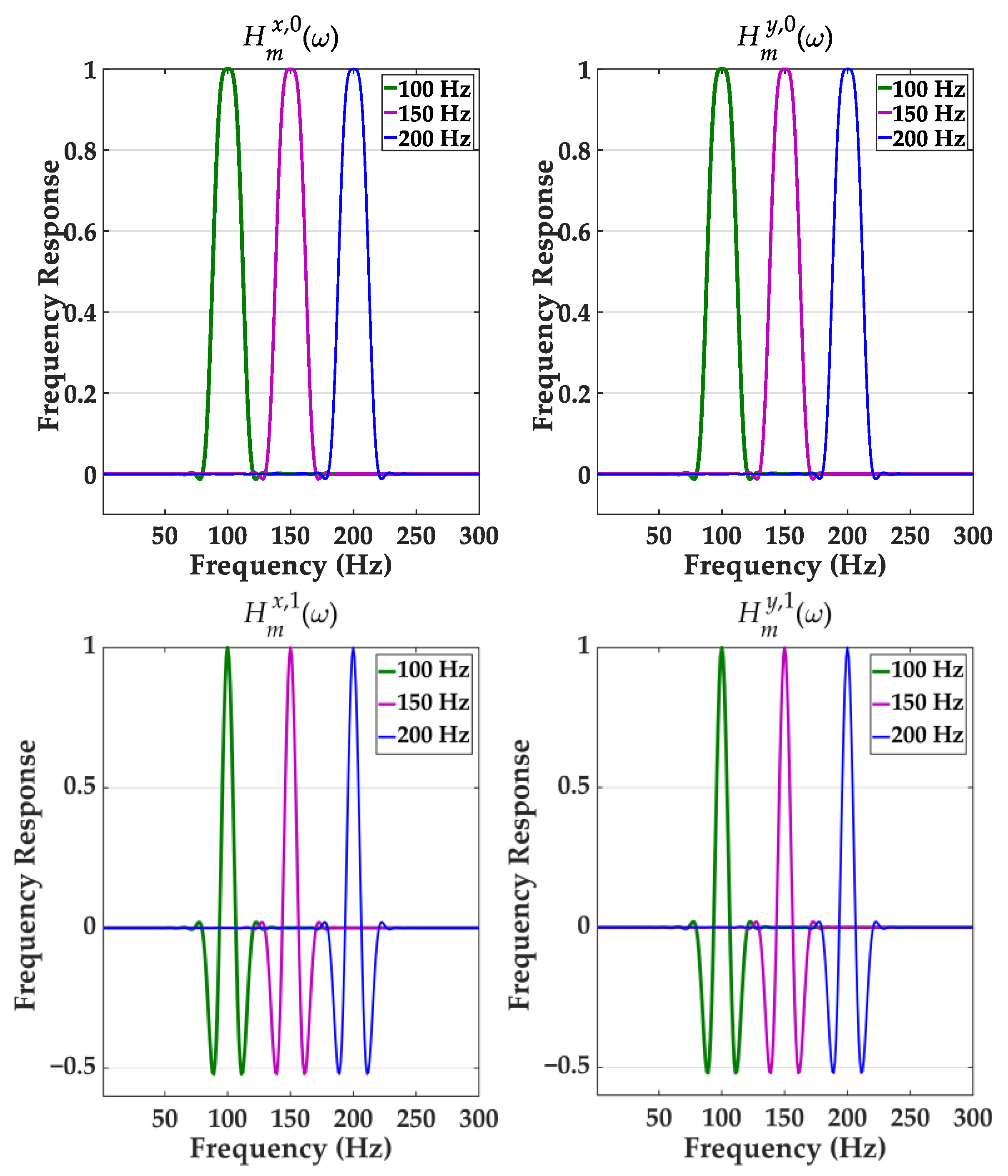
where . Figure 1 illustrates the frequency response of a filter bank considering three harmonics with preset central frequencies of 100 Hz, 150 Hz, and 200 Hz. Since multiple frequency components are simultaneously considered when constructing the Taylor expansion basis matrix for the composite modulation components, the filter bank exhibits ideal bandpass characteristics at the preset central frequencies, allowing the frequency signals to pass without attenuation. However, influenced by changes in the system’s operation state, the actual frequencies of the signal components often deviate from the preset central frequencies of the composite modulation components, making it difficult for the estimated components to achieve an ideal bandpass response near their own preset central frequencies and leading to a distortion error in the estimation results. Theoretically, is equal to which can be seen from the frequency response shown in Figure 1. Thus, the nonlinear relationship between the estimated values and the true values is determined by the frequency response below.
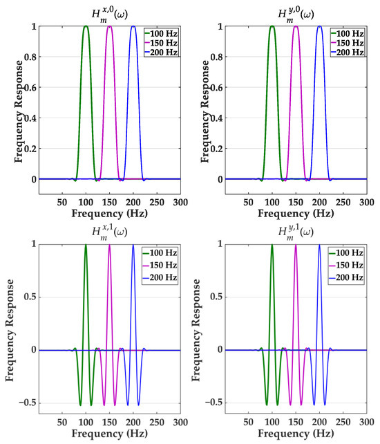
Figure 1.
Frequency response of filter bank with center frequencies of 100 Hz, 150 Hz, and 200 Hz.
4. Proposed Real-Valued Fast Estimator of Dynamic Harmonics
4.1. Proposed Real-Valued Fast Estimator Based on Estimation Error Modification
To achieve the high-precision estimation, the center frequencies of the passband of the filter bank can be typically adjusted based on the feedback from the frequency deviation estimation in an iterative sense, gradually converging to the true frequencies. However, each iteration involves multiple intermediate variable matrix calculations, including complex matrix multiplications and inversions, leading to a significant increase in computational complexity. If the accurate value of the frequency deviation can be obtained from the nonlinear relationship , the harmonic estimation errors can be directly compensated using the frequency response functions of the filters. However, is a nonlinear function, making it difficult to obtain a closed-form solution for its inverse using . Therefore, it is not possible to directly derive from .
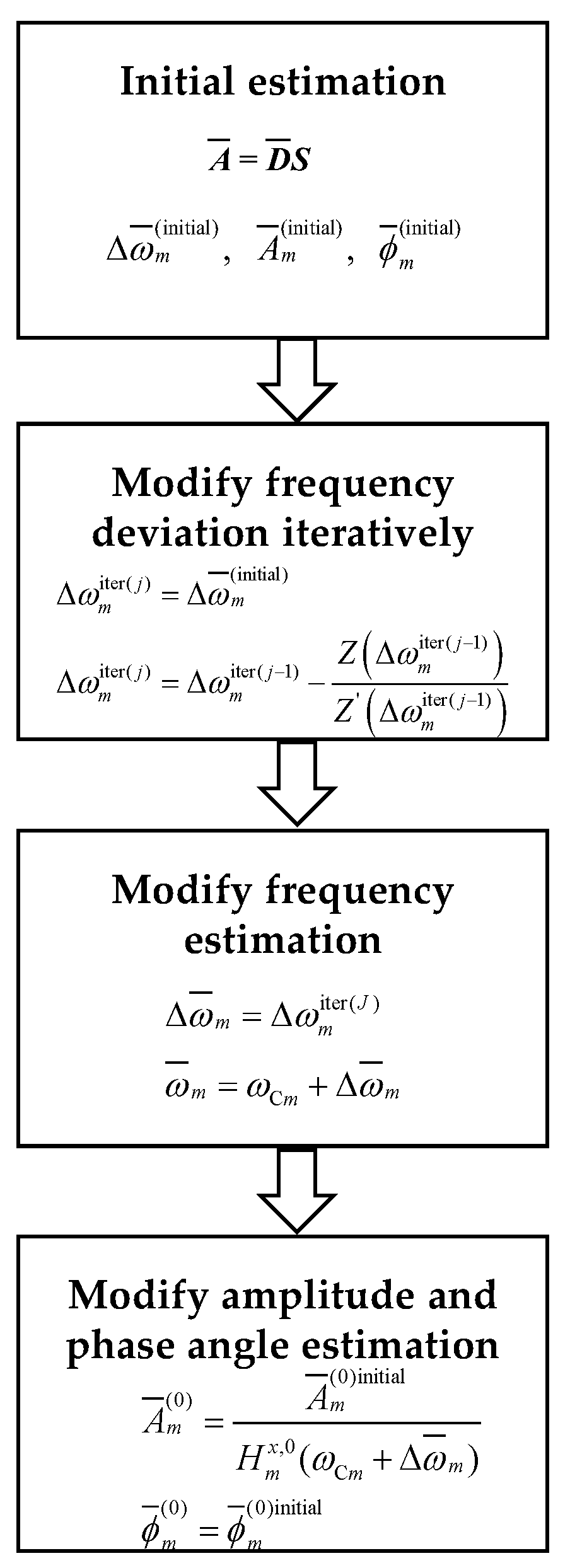
Based on the theoretical estimation error of frequency deviation discussed in Section 3.2, the nonlinear equation is constructed. A purely real-valued fast estimator for dynamic harmonics that iteratively corrects the estimated frequency deviation is proposed. This estimator leverages the frequency response functions of the filters to compensate for the estimation errors caused by frequency deviations. The specific steps are as follows:
Step 1: Establish a fitting model for the identified frequency deviation, the frequency response of the 0th-order filter, and the frequency response of the 1st-order filter.
where Q is the fitting order; and , satisfying , are the q-th order fitting parameters. These fitting parameters are calculated offline.
Step 2: Acquire the sampling sequence, and then use Equations (13) and (16) to obtain the preliminary estimation results: , and .
Step 3: Construct Equation and its derivative ; then, initialize . Use Equation (22) to iteratively correct the frequency deviation where represents the result of the j-th iteration. J is the final number of the iterations where is not the same as .
Step 4: Correct the frequency estimation results.
Then, use Equation (21) to calculate. Finally, use Equation (16) to obtain the corrected estimation results. The flowchart of the proposed estimator is shown in Figure 2.

Figure 2.
Flowchart of the proposed estimator.
4.2. Parameter Selection
4.2.1. Window Function Selection
The essence of the signal windowing is to truncate the signal. The performance of the commonly used window functions is shown in Figure 3 [33,34,35]. The rectangular window has the narrowest main lobe, but its sidelobe attenuation rate is the slowest. The sidelobe attenuation rate of the cosine window is twice that of the rectangular window, with the main lobe’s width increasing to 1.5, offering no significant advantage over the triangular window. The triangular window has a main lobe width of 2.0, but the sidelobe attenuation rate is the same as that of the cosine window. The Hanning window has a main lobe width that is twice that of the rectangular window, but its sidelobe attenuation rate is three times faster. The main lobe width of the Hamming window is the same as that of the Hanning window, but its sidelobe attenuation rate is the same as that of the rectangular window. Compared to the Hanning window, the window has a faster sidelobe attenuation rate but a wider main lobe width. The main disadvantage of the Blackman window is that its main lobe width is three times that of the rectangular window. The window has a sidelobe attenuation rate that is six times faster than that of the rectangular window, and its main lobe width is three times that of the rectangular window. The main lobe width of the Blackman–Harris window is four times that of the rectangular window, and its attenuation rate is the same as that of the rectangular window. In summary, using the window to suppress spectral leakage is reasonable, as it ensures a relatively narrower main lobe width while enabling rapid sidelobe decay. In this paper, the window was used.
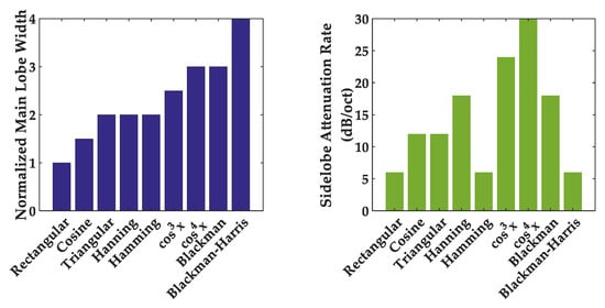
Figure 3.
Performance of the commonly used window functions.
4.2.2. Window Interval Selection
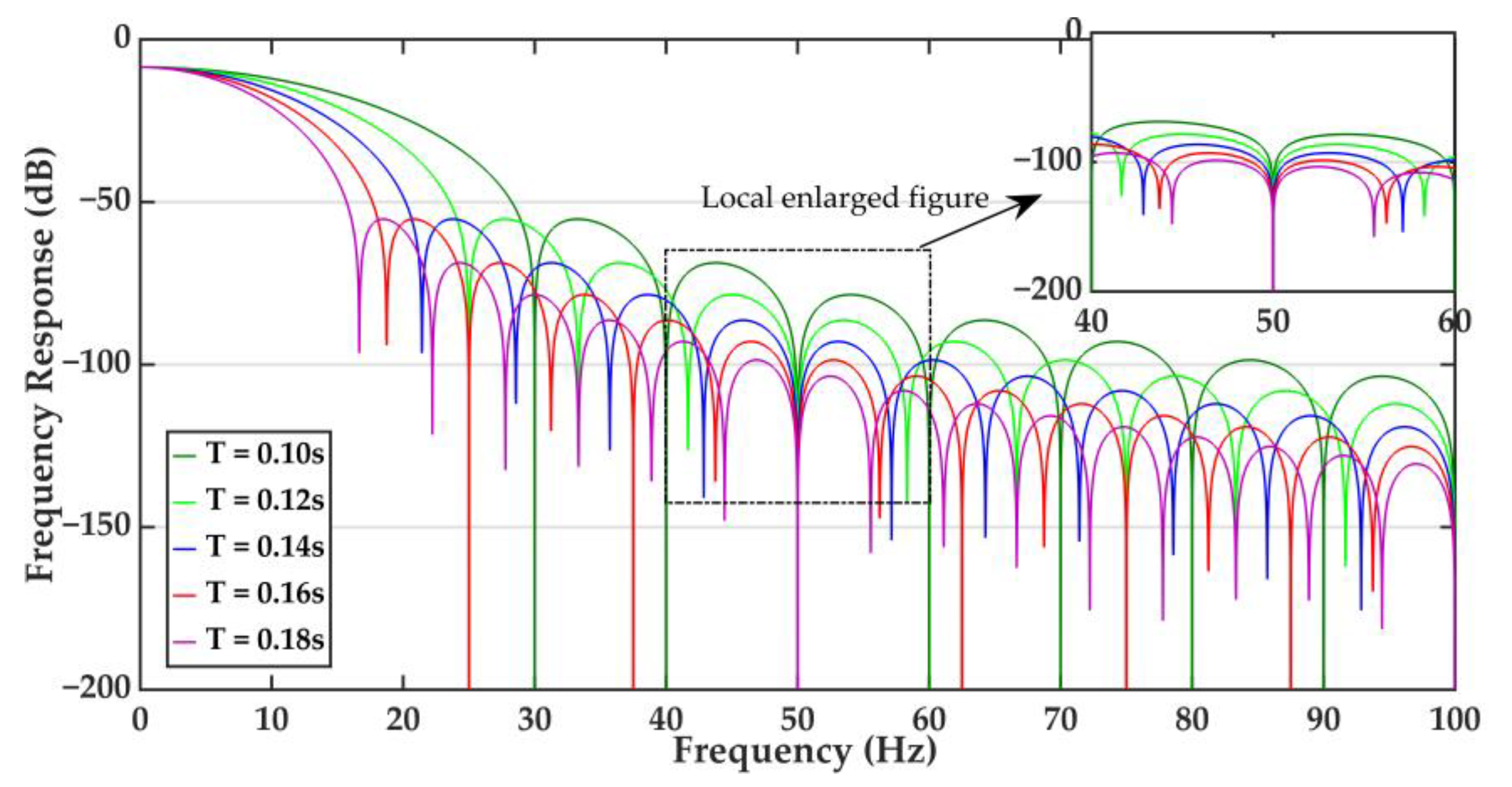
The window interval should promise that the stopband interference can be reduced to a level that is at least below the noise while being as short as possible. The noise is mainly related to the analog-to-digital conversion quantization noise and the background noise, usually assumed to be Gaussian white noise. The commonly used 16-bit analog-to-digital converter introduces a quantization noise signal-to-noise ratio (SNR) of 98.08 dB. The SNR of the background noise in the power grid signal is generally 60 dB. Therefore, it is reasonable to choose a window interval that achieves at least −100 dB of the attenuation level at the stopband interference. The frequency responses of the window with different window intervals are shown in Figure 4, and the window interval was chosen to be 0.16 s.
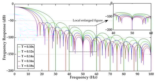
Figure 4.
Frequency responses of window with different window intervals.
4.2.3. Fitting Order Selection
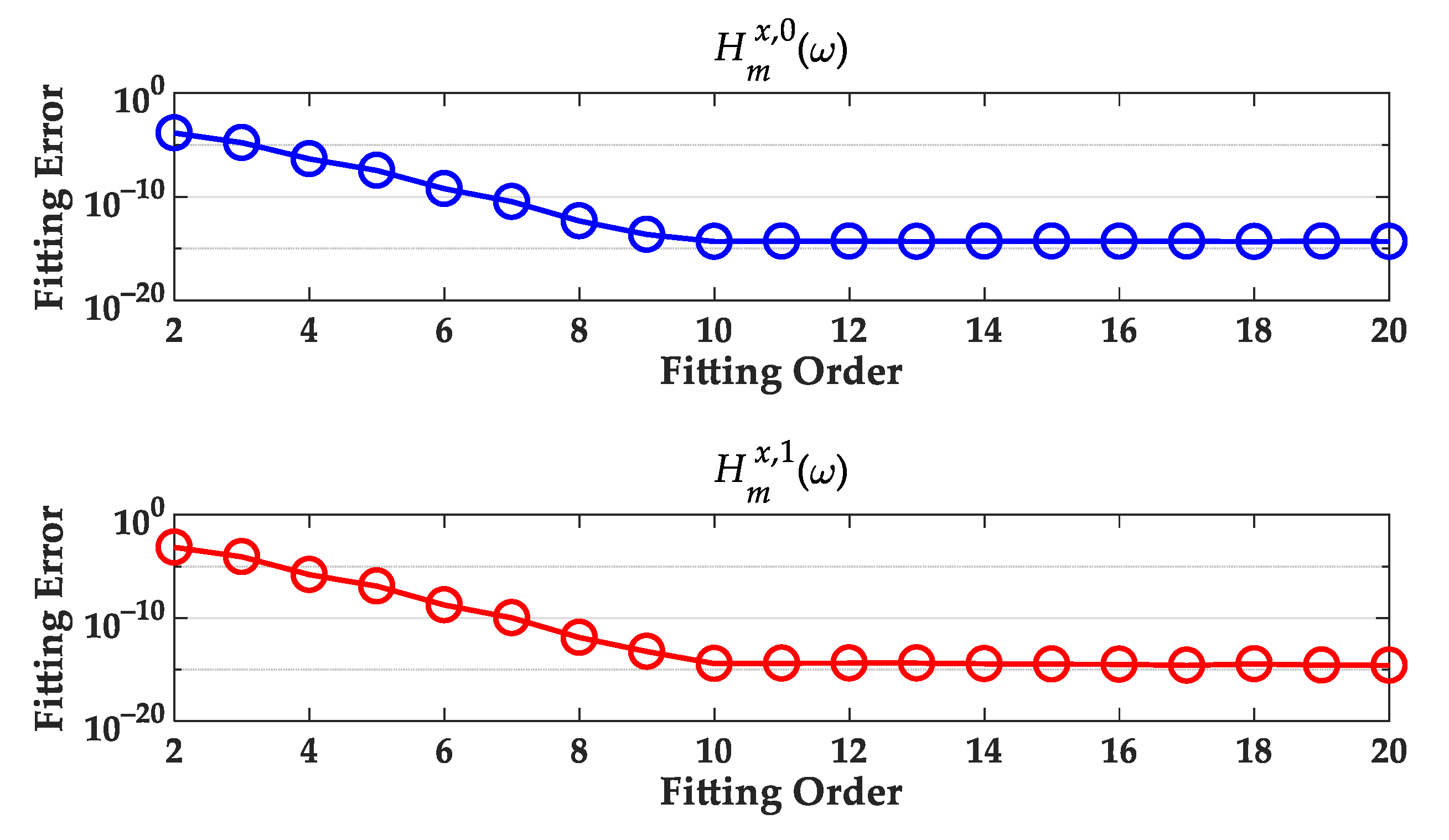
The fitting error of the passband frequency response is shown in Figure 5. When the fitting order exceeds nine, the fitting error drops below 10 × 10−14. And as the fitting order continues to increase, the fitting error does not decrease rapidly anymore. Therefore, this paper selects a fitting order of 10, i.e., Q = 10.
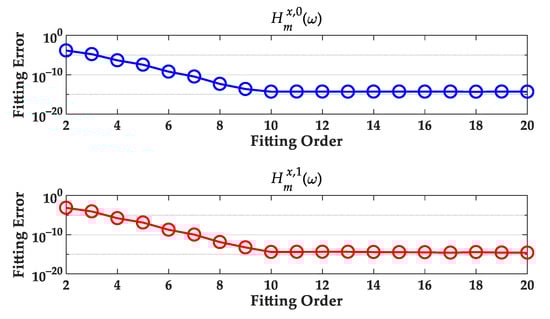
Figure 5.
Fitting errors corresponding to different fitting orders.
5. Performance Evaluation
This section verifies the dynamic harmonics estimation performance of the proposed estimator using numerical simulation signals containing fundamental components, 2nd to 50th harmonics, and noise. The sampling rate was also set to 12.8 kHz. The signal-to-noise ratio (SNR) was 98 dB. The comparison methods included IpDFT, Prony, ESPRIT, and I-TFT. IpDFT used a three-spectrum-line interpolation algorithm based on a Hanning window [18]. Prony and ESPRIT were set with an order equal to half of the window length to enhance noise resistance [21]. For I-TFT, the expansion order was set to two. The detailed parameters set is shown in Table 1.

Table 1.
Parameters of the methods.
5.1. Accuracy Evaluation
To comprehensively evaluate the accuracy of the proposed estimator, the generated numerical signals with the known amplitude, frequency, and phase angle of each harmonic and three scenarios were set up. Scenario 1 considered harmonic frequency deviation. Scenario 2 simultaneously considered the ramp change in harmonic frequency and the oscillation change in harmonic amplitude. Scenario 3 simultaneously considered the oscillation changes in harmonic frequency and the ramp changes in harmonic amplitude. The accuracy was evaluated using the estimation errors of frequency, amplitude, and phase angle, which are denoted as FE in Hz, ME in %, and PE in degree, respectively. Considering the investigation of the multiple harmonic-producing loads [36], the harmonic up to the 50th was included in the numerical signal.
5.1.1. Scenario 1
The test signal is given as follows:
where represents the initial phase angle of the mth harmonic, represents the frequency deviation of the fundamental component, and represents the frequency deviation of the mth harmonic. is set to −0.5 Hz. is set to 100, and is set to 10 for the 2nd-to-50th harmonics. is set to rad/s. The total duration of the test signal was 2 s, and the estimator reporting rate was set to be five times per second. The test was repeated 1000 times, and was set to a random value in each test.
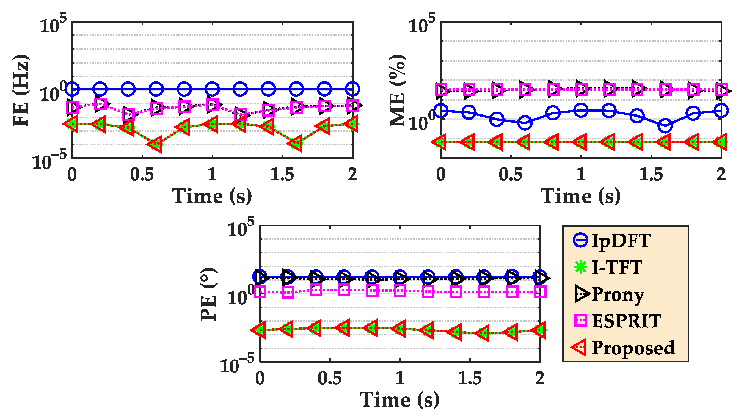
The mean estimation errors of the 1000 repeated tests of scenario 1 are shown in Figure 6. The IpDFT method exhibits the largest estimation errors due to frequency deviation. The periods of the components are not synchronized with the sampling window, leading to spectral leakage that affects the spectral line values and introduces estimation errors into the IpDFT estimation results. The Prony and ESPRIT methods show the smallest estimation errors with an FE of 1.0 × 10⁻⁶ Hz, ME of 5.8 × 10⁻⁵ %, and PE of 1.9 × 10⁻⁵ degrees, which benefited from the high degree of freedom achieved by setting a large model order. The proposed method achieves the same estimation accuracy as the I-TFT method, and its accuracy is just slightly lower than the Prony and ESPRIT methods.
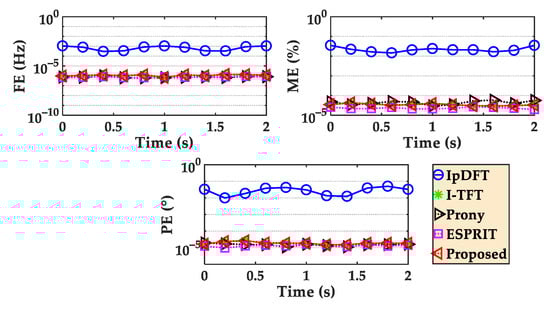
Figure 6.
Comparison of mean estimation errors in scenario 1.
5.1.2. Scenario 2
The test signal is given as follows:
where represents the initial frequency deviation of the fundamental component, represents the initial frequency deviation of the mth harmonic, and is set to −0.5 Hz. represents the frequency ramp rate of the fundamental component, represents the frequency ramp rate of the mth harmonic, and is set to 0.5 Hz/s. is set to 100, and is set to 10 for the 2nd-to-50th harmonics. represents the modulation amplitude of the amplitude oscillation, represents the modulation frequency of the amplitude oscillation, and represents the modulation phase angle of the amplitude oscillation. is set to 10 % and is set to 0.5 Hz. is set to rad/s. The total duration of the test signal was 2 s, and the estimator reporting rate was set to be five times per second. The test was repeated 1000 times. and were set to be random values in each test.
The mean estimation errors of the 1000 repeated tests of scenario 2 are shown in Figure 7. The estimation errors of the IpDFT method are larger than those in scenario 1, indicating that the harmonic, dynamic changes have a far greater impact on the estimation accuracy of IpDFT than the spectral leakage caused by non-synchronous sampling. Since the autocorrelation model also does not consider the dynamic process of the signal, the estimation errors of the Prony and ESPRIT methods increase compared to scenario 1. The proposed method and I-TFT method have the smallest estimation errors with an FE of 3.3 × 10⁻³ Hz, ME of 6.8 × 10⁻²%, and PE of 3.2 × 10⁻³ degrees, which are slightly higher than those in scenario 1.

Figure 7.
Comparison of mean estimation errors in scenario 2.
5.1.3. Scenario 3
The test signal is given as follows:
where represents the modulation amplitude of the frequency oscillation, represents the modulation frequency of the frequency oscillation, and represents the modulation phase angle of the frequency oscillation. is set to 0.5 Hz and is set to 0.5 Hz. is set to 100, and is set to 10 for the 2nd-to-50th harmonics. represents the amplitude ramp rate of each component and is set to 10%/s. is set to rad/s. The total duration of the test signal was 2 s and the estimator reporting rate was set to be five times per second. and were set to be random values in each test.
The mean estimation errors of the 1000 repeated tests of scenario 3 are shown in Figure 8. The estimation errors of the IpDFT method show no significant change compared to scenario 2. Compared to scenario 2, the estimation errors of the Prony and ESPRIT methods increase. The proposed method and the I-TFT method show the smallest estimation errors with an FE of 3.4 × 10⁻² Hz, ME of 6.5 × 10⁻¹%, and PE of 7.6 × 10⁻² degrees, which are at least ten times larger than those in scenario 2.
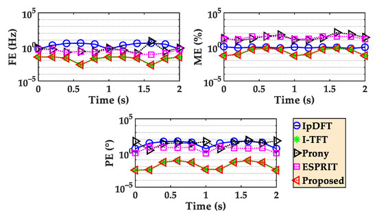
Figure 8.
Comparison of mean estimation errors in scenario 3.
5.2. Computational Time Consumption Evaluation
5.2.1. Time Consumption Comparison
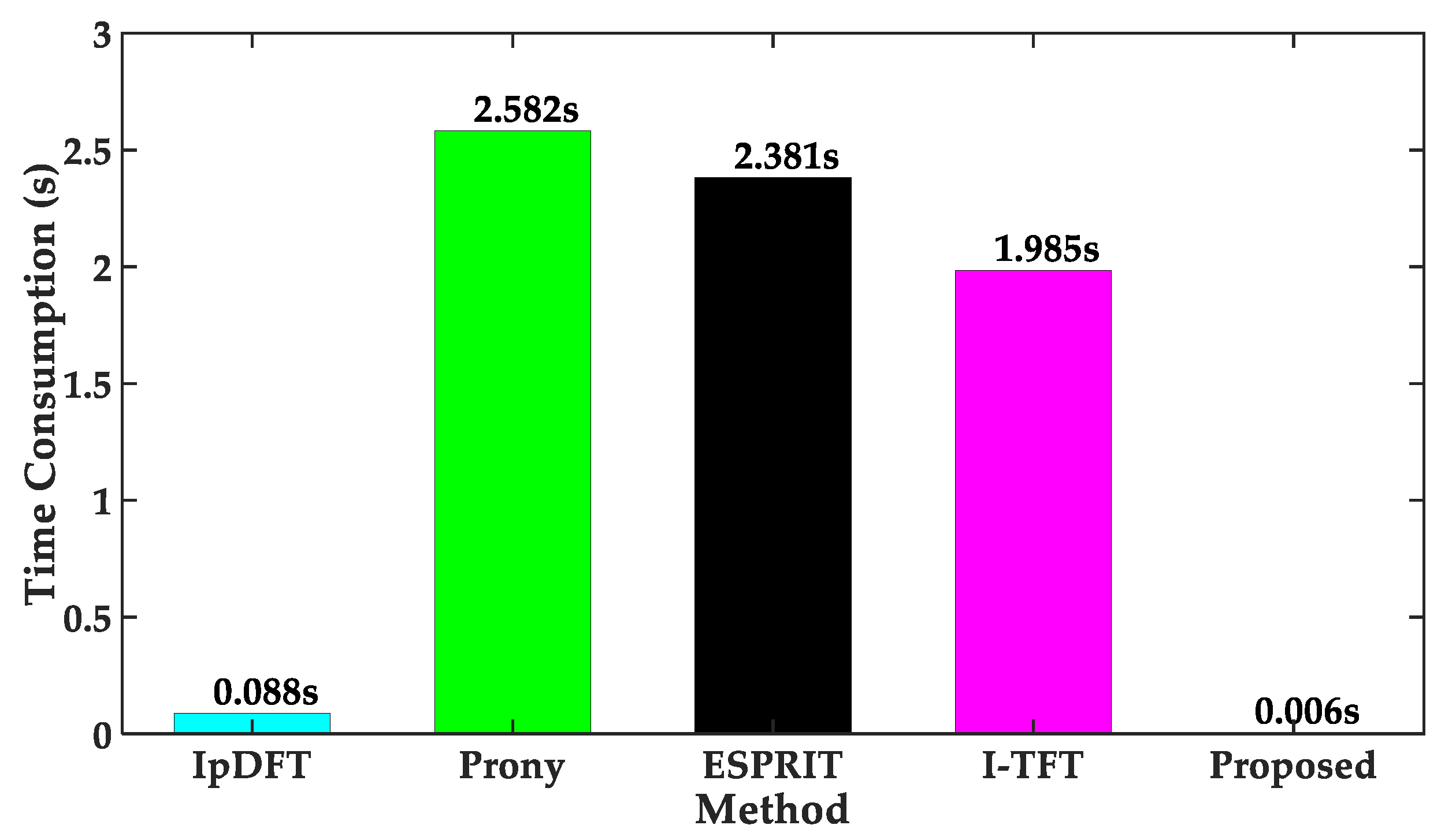
The computational time consumption of each method was tested using MATLAB 2016b on the computer with a CPU 12th Gen Intel(R) Core(TM) i7-1265U @ 2.70 GHz, RAM 32 GB, 64-bits Windows 11 operation system of surface laptop 5 manufactured in the United States. The comparison of the average time consumption of the three methods is shown in Figure 9. It can be seen that the proposed estimator achieved a computational speed-up of approximately 430, 396, and 330 times compared to the Prony method, ESPRIT method, and I-TFT method, respectively.

Figure 9.
Comparison of average time consumption.
5.2.2. Computational Complexity Analysis
The computational burden of the Prony method with a model order of primarily consists of establishing a linear prediction model , solving the polynomial root , and estimating the amplitude and phase angle, , yielding a total computational complexity of . Similarly, the total computational complexity of ESPRIT is about , which is lower than Prony. The computational burden of each iteration of the I-TFT method primarily involves the pseudo-inverse solving of the Taylor Fourier basis matrix and matrix multiplication , which is lower than both the Prony method and ESPRIT method. The computational burden of the proposed method in this paper mainly comprises the initial estimation , frequency response updates, and error compensation in each iteration process , which is significantly lower than that of the I-TFT method. Additionally, the proposed method does not require storing intermediate variables and only requires the storing of filter bank parameters and frequency response fitting parameters with a total quantity of . The proposed method has the capability for real-time application on the embedded measurement terminals with limited computational resources.
5.2.3. Implementation Time Consumption Test on Embedded Prototype
The proposed estimator was implemented on the embedded prototype, as shown in Figure 10. The signal first entered the prototype through the wiring terminal and was then converted into the 3.3 V level signal by the instrumental transformer. The transformed signal was sampled by the analog-to-digital conversion (ADC) core at a 12.8 kHz sampling rate and then was fast written into flash memory through FPGA. Then, the proposed estimator was implemented in the C6748 DSP module. It should be noted that a high-performance microcontroller or DSP can be alternatively used instead of an FPGA to achieve high-speed sampling. However, the sampling process would interrupt the measurement algorithm that the DSP is currently executing, thereby additionally increasing the computational load of the DSP. On the other hand, using an FPGA for sampling control allows the DSP to directly read the buffered sampling sequence from flash memory only when it needs to execute the measurement algorithm, enabling the DSP to perform the measurement algorithm more quickly. Thus, FPGA was used for the high-speed sampling in this paper. To estimate 50 harmonics, the initial estimation step takes around 20 milliseconds (ms). The frequency deviation calculation step and estimation modification step take around 0.5 ms. The computational load rate for executing the proposed estimator and estimating 50 harmonics was approximately 2.05%.
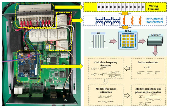
Figure 10.
Implementation scheme of the proposed estimator on the embedded prototype.
6. Discussion
Based on the test results, the IpDFT method can barely achieve the high-precision estimation of dynamic harmonics due to static signal model and spectral leakage issues. The Prony and ESPRIT methods, by setting a higher model order with greater degrees of freedom, can improve the estimation accuracy of dynamic harmonics to a certain extent. However, the estimation error of the Prony method remains higher than that of the I-TFT method and the proposed method. The comparison of different methods and their performances is briefly summarized in Table 2.
Table 2.
Summary of performance comparisons of different methods.
Due to the inability to completely suppress stopband interference signals when the preset center frequencies of the filter bank deviate from the true frequencies of the signals, estimation errors caused by stopband interference are introduced into the estimation results and further propagate into the correction process, reducing the modification accuracy. In this paper, the interference issue is mitigated to a certain extent by applying windowing processing and reasonably selecting windowing parameters. The proposed method achieves a substantial increase in computational speed and a significant reduction in memory overhead at the expense of a small sacrifice in estimation accuracy. Therefore, it can be considered that the negative impact of interference errors on the proposed method is minor or negligible.
From the signal estimation model to the estimation algorithm, there are no complex-valued operations involved, and it does not rely on native support for complex-valued operations in embedded measurement devices. It can be directly ported and applied to various types of embedded systems without the need for the special real-valued processing of complex-valued programs based on the specific type of embedded system. There are no special requirements for the selection of embedded systems, which enhances the versatility of the estimator. To further enhance the practical applicability of the proposed algorithm, it is necessary to improve its execution process and optimize the estimation parameters based on the wideband signal characteristics of monitoring targets.
7. Conclusions
To solve the problem of the traditional dynamic harmonics estimation methods that result in a heavy computational burden and large memory space, this paper proposes a purely real-valued fast estimator for dynamic harmonics. Numerical simulation testing results demonstrate that the proposed estimator achieves the high-accuracy estimation of dynamic harmonics under various scenarios, including frequency deviation, frequency ramp, frequency oscillation, amplitude ramp, and amplitude oscillation. The proposed estimator avoids the complicated computation of complex-valued matrices and the trigonometric function computations, significantly reducing computational complexity and memory space consumption. Testing results show that the proposed estimator achieves a computational speed-up of approximately 430, 396, and 330 times compared to the Prony method, ESPRIT method, and I-TFT method, respectively. The computational load rate for executing the proposed estimator and estimating 50 harmonics using the C6748 DSP-based embedded prototype is only approximately 2.05%, demonstrating the application potential of the proposed estimator in the high-precision online measurement of dynamic harmonics in power grids.
To further enhance the computational efficiency of the algorithm, additional research is necessary to investigate the potential of employing the dynamic harmonic estimator with shorter time windows while maintaining estimation accuracy.
Author Contributions
Conceptualization, Z.J. and X.L.; methodology, C.Z. and H.S.; validation, B.G.; formal analysis, X.L.; data curation, H.S. and H.W.; writing—original draft preparation, Z.J. and X.L.; writing—review and editing, C.Z. and H.W. All authors have read and agreed to the published version of the manuscript.
Funding
This research was funded by the State Grid Shanghai Municipal Electric Power Company Science and Technology Project: 520921240003.
Data Availability Statement
The data are available from the corresponding author upon reasonable request.
Conflicts of Interest
Authors Xiao Luo, Haoqiang Wu and Boyang Gao were employed by State Grid Shanghai Municipal Electric Power Company. The remaining authors declare that the research was conducted in the absence of any commercial or financial relationships that could be construed as a potential conflict of interest.
Abbreviations
| HVDC | High-Voltage Direct Current |
| FFT | Fast Fourier transform |
| IpDFT | Interpolated DFT |
| ESPRIT | Estimation of signal parameters via rotational invariance technique |
| TFT | Taylor Fourier transform |
| I-TFT | Iterative TFT |
| MCU | Microcontroller unit |
| RAM | Random Access Memory |
| SNR | Signal-to-noise ratio |
| FE | Frequency error |
| ME | Magnitude error |
| PE | Phase angle error |
| ADC | Analog-to-digital conversion |
| FPGA | Field-Programmable Gate Array |
| DSP | Digital Signal Processor |
| Variables and Paraments | |
| The amplitude of the mth harmonic at time t | |
| The frequency of the mth harmonic at time t | |
| The phase of the mth harmonic at time t | |
| M | The number of harmonics |
| Denotes the th derivative of | |
| The initial amplitude | |
| The amplitude rate of change | |
| The th derivative of | |
| The initial phase angle | |
| The frequency deviation | |
| , | The composite modulation components that simultaneously incorporate both the amplitude and frequency dynamics |
| , | The kth derivatives of and |
| The sampling period | |
| The diagonal matrix of the kth order expansion time coefficients | |
| , | The vectors of trigonometric expansion basis functions |
| The window function-weighted diagonal matrix | |
| , | The estimator parameter vectors for the derivatives of the composite modulation components |
| , | The frequency response of the filter and |
| , | The q-th order fitting parameters |
| The result of the j-th iteration | |
| The initial phase angle of the mth harmonic | |
| The frequency deviation of the fundamental component | |
| The frequency deviation of the mth harmonic | |
| The frequency ramp rate of the fundamental component | |
| The frequency ramp rate of the mth harmonic | |
| The modulation amplitude of the amplitude oscillation | |
| The modulation frequency of the amplitude oscillation | |
| The modulation phase angle of the amplitude oscillation | |
| The modulation amplitude of frequency oscillation | |
| The modulation frequency of frequency oscillation | |
| The modulation phase angle of frequency oscillation | |
| The amplitude ramp rate of each component |
References
- Fan, Y.; Xu, F.; Wang, C.; Shu, Q. A Harmonic Impedance on Utility Side Estimation Method Based on Laplace Mixture Model. IEEE Trans. Power Del. 2024, 39, 1774–1782. [Google Scholar] [CrossRef]
- Xu, Q.; Zhu, F.; Jiang, W.; Pan, X.; Li, P.; Zhou, X.; Wang, Y. Efficient Identification Method for Power Quality Disturbance: A Hybrid Data-Driven Strategy. Processes 2024, 12, 1395. [Google Scholar] [CrossRef]
- Ji, K. Harmonic Power Modeling for Converter-Driven Stability Study. IEEE Trans. Power Del. 2023, 38, 3968–3979. [Google Scholar] [CrossRef]
- Li, Y.; Sun, Y.; Wang, Q.; Sun, K.; Li, K.; Zhang, Y. Probabilistic harmonic forecasting of the distribution system considering time-varying uncertainties of the distributed energy resources and electrical loads. Appl. Energy 2023, 329, 120298. [Google Scholar] [CrossRef]
- Xia, Y.; Xu, Y.; Feng, X. Hierarchical Coordination of Networked-Microgrids Toward Decentralized Operation: A Safe Deep Reinforcement Learning Method. IEEE Trans. Sustain. Energy 2024, 15, 1981–1993. [Google Scholar] [CrossRef]
- Shan, P.; Sun, Y.; Song, Y.; Zhang, F.; Li, Y.; Sun, K. Adaptive Parameter Tuning and Virtual Impedance Injection Control for Coupled Harmonic Mitigation of Photovoltaic Converter. IEEE Trans. Power Electron. 2025, 40, 162–175. [Google Scholar] [CrossRef]
- Zou, Y.; Xu, Y.; Li, J. Aggregator-Network Coordinated Peer-to-Peer Multi-Energy Trading via Adaptive Robust Stochastic Optimization. IEEE Trans. Power Syst. 2024, 39, 7124–7137. [Google Scholar] [CrossRef]
- Taghvaie, A.; Warnakulasuriya, T.; Kumar, D.; Zare, F.; Sharma, R.; Vilathgamuwa, D.M. A Comprehensive Review of Harmonic Issues and Estimation Techniques in Power System Networks Based on Traditional and Artificial Intelligence/Machine Learning. IEEE Access 2023, 11, 31417–31442. [Google Scholar] [CrossRef]
- Mariscotti, A.; Mingotti, A. The Effects of Supraharmonic Distortion in MV and LV AC Grids. Sensors 2024, 24, 2465. [Google Scholar] [CrossRef]
- Jiang, X.; Yi, H.; Zhuo, F.; Li, Y. An Adaptive Stabilization Strategy for Harmonic Oscillation of SAPF Interacted With Nonlinear Load and Grid Impedance. IEEE Trans. Ind. Electron. 2024, 71, 9044–9054. [Google Scholar] [CrossRef]
- Zhang, Z.; Yi, H.; Zhuo, F.; Li, Y.; Jiang, X. Harmonic oscillation analysis and stabilization method comparison of shunt active power filter in full compensation mode. IET Power Electron. 2024, 17, 1145–1158. [Google Scholar] [CrossRef]
- Li, Y.; Sun, Y.; Li, K.; Sun, K.; Liu, Z.; Xu, Q. Harmonic modeling of the series-connected multi-pulse rectifiers under unbalanced conditions. IEEE Trans. Ind. Electron. 2023, 70, 6494–6505. [Google Scholar] [CrossRef]
- Li, G.; Ma, F.; Wu, C.; Li, M.; Guerrero, J.; Wong, M. A Generalized Harmonic Compensation Control Strategy for Mitigating Subsynchronous Oscillation in Synchronverter Based Wind Farm Connected to Series Compensated Transmission Line. IEEE Trans. Power Syst. 2023, 38, 2610–2620. [Google Scholar] [CrossRef]
- Xiao, H.; Li, Y.; Duan, X. Enhanced Commutation Failure Predictive Detection Method and Control Strategy in Multi-Infeed LCC-HVDC Systems Considering Voltage Harmonics. IEEE Trans. Power Syst. 2021, 36, 81–96. [Google Scholar] [CrossRef]
- Wang, L.; Yao, W.; Xiong, Y.; Shi, Z.; Wen, J. Commutation Failure Analysis and Prevention of UHVDC System With Hierarchical Connection Considering Voltage Harmonics. IEEE Trans. Power Del. 2022, 37, 3142–3154. [Google Scholar] [CrossRef]
- Demin, S.; Barbie, E.; Heistrene, L.; Belikov, J.; Petlenkov, E.; Levron, Y.; Baimel, D. Implementation of Series Resonance-Based Fault Current Limiter for Enhanced Transient Stability of Grid-Connected Photovoltaic Farm. Electronics 2024, 13, 2987. [Google Scholar] [CrossRef]
- Aleixo, R.R.; Lomar, T.S.; Silva, L.R.M.; Monteiro, H.L.M.; Duque, C.A. Real-Time B-Spline Interpolation for Harmonic Phasor Estimation in Power Systems. IEEE Trans. Instrum. Meas. 2022, 71, 9004009. [Google Scholar] [CrossRef]
- Wu, H.; Song, H.; Bai, Y.; Fan, L.; Jin, J.; Xing, J. Interpolated DFT Algorithm for Frequency Estimation by Using Maximum Sidelobe Decay Windows. IEEE Access 2022, 10, 95748–95762. [Google Scholar] [CrossRef]
- Afrandideh, S. A Modified DFT-Based Phasor Estimation Algorithm Using an FIR Notch Filter. IEEE Trans. Power Del. 2023, 38, 1308–1315. [Google Scholar] [CrossRef]
- Matusiak, A.; Borkowski, J.; Mroczka, J. Noniterative method for frequency estimation based on interpolated DFT with low-order harmonics elimination. Measurement 2022, 196, 111241. [Google Scholar] [CrossRef]
- Khodaparast, J.; Fosso, O.B.; Molinas, M. Phasor Estimation by EMD-Assisted Prony. IEEE Trans. Power Del. 2022, 37, 4736–4748. [Google Scholar] [CrossRef]
- Rao, K.S.; Shubhanga, K.N. A Comparison of SVD-Augmented Prony Algorithms for Noisy Power System Signals. IEEE Access 2023, 11, 143457–143474. [Google Scholar] [CrossRef]
- Anshuman, A.; Jena, M.K.; Panigrahi, B.K. Linear Estimation of Low-Frequency Modal Oscillations Parameters Through Nonlinear Characterization. IEEE Trans. Instrum. Meas. 2023, 72, 9004404. [Google Scholar] [CrossRef]
- Eranti, P.K.; Barkana, B.D. An Overview of Direction-of-Arrival Estimation Methods Using Adaptive Directional Time-Frequency Distributions. Electronics 2022, 11, 1321. [Google Scholar] [CrossRef]
- Srivastava, A.K.; Tiwari, A.N.; Singh, S.N. Harmonic and Interharmonic Estimation Using Poincare Filtering Assisted ESPRIT Method. IEEE Trans. Ind. Appl. 2023, 59, 4859–4867. [Google Scholar] [CrossRef]
- Serna, J.A.d.l.O. Dynamic Harmonic Analysis With FIR Filters Designed With O-Splines. IEEE Trans. Circuits Syst. I-Regul. Pap. 2020, 67, 5092–5100. [Google Scholar] [CrossRef]
- Singh, A.; Jaafari, K.A.; Parida, S.K.; Al-Durra, A.; Zeineldin, H.H.; El-Saadany, E.F. Dynamic Synchrophasor Estimation Algorithm Using Taylor Weighted Least Square Method With Harmonic Input Model. IEEE Trans. Ind. Appl. 2023, 59, 7417–7427. [Google Scholar] [CrossRef]
- Jin, Z.; Zhang, H.; Terzija, V. An Embedded Estimator for Online Harmonic Monitoring in Power-Electronic Grids. IEEE Trans. Smart Grid 2022, 13, 4677–4689. [Google Scholar] [CrossRef]
- Shekar, H.B.; Bhat, S.S.; Shetty, R. Edge Detection in Gray-Scale Images Using Partial Sum of Second-Order Taylor Series Expansion. SN Comput. Sci. 2024, 5, 197. [Google Scholar] [CrossRef]
- Paux, J.; Morin, L.; Gélébart, L. A Discrete Sine-Cosine Transforms Galerkin Method for the Conductivity of Heterogeneous Materials With Mixed Dirichlet/Neumann Boundary Conditions. Int. J. Numer. Meth. Eng. 2024, 126, e7615. [Google Scholar] [CrossRef]
- Zhao, R. Least lp-norm design of complex exponential structure variable fractional delay FIR filters. Signal Process. 2024, 218, 109387. [Google Scholar] [CrossRef]
- Li, X.; Li, Y.N.; Zhang, L.X.; Zhao, J. Inference for high-dimensional linear expectile regression with de-biasing method. Comput. Stat. Data An. 2024, 198, 107997. [Google Scholar] [CrossRef]
- Prabhu, K.M.M. Window Functions and Their Applications in Signal Processing; Taylor & Francis Group: Oxford, UK, 2013; p. 93. [Google Scholar]
- Das, M.; Kumar, R.; Sahana, B.C. Implementation of effective hybrid window function for E.C.G signal denoising. Trait. Signal 2020, 37, 119–128. [Google Scholar] [CrossRef]
- Justo, J.F.; Beccaro, W. Generalized Adaptive Polynomial Window Function. IEEE Access 2020, 8, 187584–187589. [Google Scholar] [CrossRef]
- Cicek, A.; Erenoglu, A.K.; Erdinc, O.; Bozkurt, A.; Tascikaraoglu, A.; Catalao, J.P.S. Implementing a Demand Side Management Strategy for Harmonics Mitigation in a Smart Home Using Real Measurements of Household Appliances. Int. J. Electr. Power Energy Syst. 2021, 125, 106528. [Google Scholar] [CrossRef]


Disclaimer/Publisher’s Note: The statements, opinions and data contained in all publications are solely those of the individual author(s) and contributor(s) and not of MDPI and/or the editor(s). MDPI and/or the editor(s) disclaim responsibility for any injury to people or property resulting from any ideas, methods, instructions or products referred to in the content. |
© 2025 by the authors. Licensee MDPI, Basel, Switzerland. This article is an open access article distributed under the terms and conditions of the Creative Commons Attribution (CC BY) license (https://creativecommons.org/licenses/by/4.0/).