Abstract
Accurate prediction of methane concentration in mine roadways is crucial for ensuring miner safety and enhancing the economic benefits of mining enterprises in the field of coal mine safety. Taking the Buertai Coal Mine as an example, this study employs laser methane concentration monitoring sensors to conduct precise real-time measurements of methane concentration in coal mine roadways. A prediction model for methane concentration in coal mine roadways, based on an Improved Black Kite Algorithm (IBKA) coupled with Informer-BiLSTM, is proposed. Initially, the traditional Black Kite Algorithm (BKA) is enhanced by introducing Tent chaotic mapping, integrating dynamic convex lens imaging, and adopting a Fraunhofer diffraction search strategy. Experimental results demonstrate that the proposed improvements effectively enhance the algorithm’s performance, resulting in the IBKA exhibiting higher search accuracy, faster convergence speed, and robust practicality. Subsequently, seven hyperparameters in the Informer-BiLSTM prediction model are optimized to further refine the model’s predictive accuracy. Finally, the prediction results of the IBKA-Informer-BiLSTM model are compared with those of six reference models. The research findings indicate that the coupled model achieves Mean Absolute Errors (MAE) of 0.00067624 and 0.0005971 for the training and test sets, respectively, Root Mean Square Errors (RMSE) of 0.00088187 and 0.0008005, and Coefficient of Determination (R2) values of 0.9769 and 0.9589. These results are significantly superior to those of the other compared models. Furthermore, when applied to additional methane concentration datasets from the Buertai Coal Mine roadways, the model demonstrates R2 values exceeding 0.95 for both the training and test sets, validating its excellent generalization ability, predictive performance, and potential for practical applications.
1. Introduction
As the primary cause of coal mine accidents, gas explosions account for approximately 50% of major mining disasters in China [1,2,3]. Mine gas, a collection of combustible gasses released during coal mining, primarily consists of methane (CH4), which accounts for over 90% of its composition [4]. Accurate monitoring of gas concentrations enables the timely detection of potential hazards underground, allowing for prompt evacuation and ensuring the safety of personnel and equipment [5,6]. However, traditional monitoring techniques are limited to real-time measurements of current gas concentrations and struggle to effectively predict future trends [7]. In light of this, developing efficient gas concentration prediction models to enable early warning and preventive measures has become a crucial research direction in preventing coal mine gas explosion accidents [8,9].
Currently, the primary monitoring methods employed include manual inspection and online surveillance [10]. However, with the advent of the big data era and advancements in artificial intelligence (AI) technology, numerous scholars have turned their attention to the field of intelligent coal mine detection and prediction, utilizing interdisciplinary approaches that integrate AI technology [11], sensor detection technology [12,13], and other disciplines to monitor methane gas concentrations in coal mines. These methods have, to some extent, improved monitoring accuracy, yet they still face several challenges. The effectiveness of AI-based monitoring often relies on vast amounts of historical data, and monitoring in coal mine environments can frequently yield significant deviations. Although sensor technology enables real-time monitoring of methane concentrations, traditional point sensors typically only detect gas concentrations in localized areas, making it difficult to comprehensively reflect the methane distribution throughout the entire mine. Inaccurate monitoring of methane concentrations in coal mine roadways significantly impacts the accuracy of future methane concentration predictions, leading to substantial prediction errors [14,15,16].
With the evolution of technology, the integration of coal mine roadway methane concentrations with artificial intelligence, big data, machine learning, and metaheuristic algorithms has emerged as a research hotspot. Numerous scholars have conducted extensive research in this area. For instance, Nie, Z. et al. [17] studied methane diffusion theory and the characteristics of coal mine environments, employing the Gaussian plume model to simulate methane diffusion patterns in coal mine roadways. They proposed an optimized methane prediction model based on a combination of genetic algorithms and BP neural networks. This model, characterized by low computational complexity and high prediction accuracy, can enhance its reliability through continuous machine learning from daily monitoring data, providing a novel technical solution for intelligent monitoring of coal mine roadway environments. Guo, R. et al. [18] introduced an algorithm that combines information fusion technology with a genetic algorithm-support vector machine (GA-SVM). This algorithm initially uses information fusion techniques to analyze and reconstruct the correlation of raw methane concentration data. Subsequently, the genetic algorithm (GA) is employed to optimize the selection of the penalty factor C and regression parameter w in the support vector machine (SVM), thereby constructing a multi-sensor prediction model for coal mine methane concentrations. Zhiqiang Luo et al. [19] proposed a methane concentration prediction model based on multi-features and the eXtreme Gradient Boosting (XGBoost). This model integrates historical methane concentrations, temperature, wind speed, and other features, leveraging XGBoost’s gradient boosting algorithm to accelerate decision tree training. Experimental results demonstrate that this approach achieves lower prediction errors and faster training speeds compared to existing deep learning models. Fu, H. et al. [20] developed a multi-sensor methane concentration prediction model based on a deep Long Short-Term Memory network (LSTM). They first utilized the Pearson correlation coefficient method to select variables strongly correlated with methane concentrations as model input parameters, reducing the input data size and complexity. Following this, they performed multivariate phase space reconstruction and employed a random search algorithm to automatically optimize the LSTM network hyperparameters, establishing an optimal parameter multi-sensor time series dynamic prediction model. Although these studies have successfully constructed methane concentration prediction models for coal mine roadways, the prediction accuracy is still constrained, and the generalization ability and adaptability of the models require further validation.
Intelligent optimization algorithms, which simulate collective behaviors observed in nature such as bird flocks, fish schools, and ant colonies, offer novel approaches for solving complex problems [21,22,23,24]. Compared to traditional algorithms, intelligent optimization algorithms, through their ingenious designs, strike a balance between avoiding local optima and ensuring convergence to global optima. This balance enables them to demonstrate efficiency and precision in practical problem-solving, especially when confronted with challenges that are complex, dynamic, and information-incomplete. In this context, scholars have successively proposed a series of innovative optimization algorithms, including Particle Swarm Optimization (PSO) [25], Sparrow Search Algorithm (SSA) [26], Emperor Penguin Optimization (EPO) [27], Harris Hawks Optimization (HHO) [28], Sailfish Optimization (SFO) [29], Grey Wolf Optimizer (GWO) [30], and Black Kite Algorithm (BKA) [31]. These algorithms do not require specific assumptions about the problem model; instead, they progressively approximate the optimal solution by continuously exploring the search space and leveraging the problem’s characteristics. Their gradient-free nature allows them to handle problems lacking explicit gradient information or continuous derivatives, showcasing greater flexibility and robustness. However, intelligent optimization algorithms also face challenges such as local optimum stagnation and premature convergence [32,33,34,35]. To address these issues, numerous scholars have improved the algorithms from various perspectives. Among these, the application of optical phenomena has emerged as a new research hotspot [36,37]. For instance, Long, W. et al. [36] innovatively introduced the Lens Imaging Learning (LIL) operator, aimed at maintaining population diversity and helping the algorithm escape local optima. The effectiveness of the LIL-HHO algorithm was validated through 85 benchmark functions, including 25 classic functions and 30 complex functions from CEC2014, as well as 21 feature selection problems. Zhang, L. et al. [37] proposed the Adaptive Lens Imaging Enhanced Chimpanzee-based Hierarchical Optimization Algorithm (ALI-CHoASH) for solving optimal feature subset search and optimal classification problems. To address the issue of insufficient diversity in chimpanzee populations during later iterations, an adaptive lens imaging reverse learning strategy was designed, effectively preventing the algorithm from falling into local optima.
Time series represent collections of data ordered by time, which can be observed and collected at any time interval [38,39,40]. Time series data are categorized into univariate and multivariate types. Univariate time series involve changes in a single variable over time, with an observation value at each time point. In univariate time series forecasting [41,42], predictions of future values rely solely on the historical data of that variable. Conversely, multivariate time series encompass changes in two or more variables over time, each with corresponding observation values at each time point. In multivariate time series forecasting [43,44,45], the historical data of other variables are utilized to predict the future values of a specific variable. Specialized time series models are typically required to process time series data. However, there is a paucity of research on the application of time series models for predicting univariate time series data in the coal mining industry [46].
In this study, three roadways in the Buertai coal mine, namely, a 1400 m return road in the 12-coal three-panel area, a 1500 m return road in the 12-coal total return road, and a 460 m return road in the 42-coal two-panel area, are taken as the objects of the study. The sources of gas in the above roadways mainly include desorption and emergence of coal seam gas, migration of gas from neighboring coal seams, and release of gas during mining operations. These sources of gas are characterized by significant fluctuations in gas concentration during the roadway preparation and production operations. In the preparation of the roadway, the gas concentration is mainly influenced by the natural desorption and diffusion of coal seam gas, especially the enhanced effect of gas flow after the release of ground stress [47]. In addition, the migration of gas from neighboring coal seams to the roadway through inter-seam fissures and tectonic channels also constitutes an important source of gas concentration. In production operation roadways, the mining process leads to the destruction of the coal body and a significant increase in the rate of gas release, especially in high gas areas or when mining thick coal seams, the gas concentration may rapidly reach dangerous levels. In addition, high-intensity operations of coal miners and roadheaders can exacerbate the release and accumulation of gas, increasing the burden on the roadway ventilation system [48].
In summary, this study proposes an IBKA-Informer-BiLSTM model for predicting gas concentrations in coal mine roadways. The Improved Black-Winged Kite Algorithm (IBKA) is enhanced through the incorporation of Tent chaotic mapping, a dynamic convex lens imaging learning strategy, and a Fraunhofer diffraction search strategy. Combined with the Informer-BiLSTM model, it optimizes seven hyperparameters, including the number of hidden layers, learning rate, and regularization coefficient. The dataset of gas concentrations in Buertai Coal Mine roadways is randomly split into training and testing sets in a 7:3 ratio. An IBKA-Informer-BiLSTM model for predicting gas concentrations in coal mine roadways is established, and its prediction results are compared with those of six other models: LSTM, BiLSTM, Informer, Autoformer, LR, and XGBoost. This comparison validates the prediction accuracy of the proposed model. Finally, the generalization ability of the model is further verified using two additional datasets of gas concentrations from the Buertai Coal Mine (Shenhua Shendong Coal Group Corporation Limited, Hohhot, China).
2. Theoretical Foundation Research
2.1. Improved Black-Winged Kite Algorithm
2.1.1. Basic Black-Winged Kite Algorithm
The Basic Black-winged Kite Algorithm (BKA) is an optimization algorithm inspired by the foraging behavior of black-winged kite birds in nature, primarily designed to address continuous optimization problems [49,50]. The foraging behavior of black-winged kites in the wild exhibits a certain degree of randomness and exploratory nature. This algorithm draws inspiration from the wisdom of black-winged kites in skillfully balancing the “exploration” and “exploitation” strategies during hunting, aiming to efficiently traverse the solution space and, thus, achieve precise approximation of the global optimal solution. Similarly to most optimization algorithms, it uniformly distributes the position of each black-winged kite, with the population initialization position expressed as shown in Equation (1).
where I ∈ 1,2, …, N; BKlb and BKub represent the lower and upper bounds, respectively, for the j-th dimension of the black-winged kite; and rand denotes a random number within the interval [0,1].
The mathematical model for the attack behavior of black-winged kites is expressed as shown in Equation (2).
where and represent the positions of the i-th black-winged kite in the j-th dimension at the (t + 1)-th iteration step, respectively; r is a random number between 0 and 1; g is a constant with a value of 0.9; T denotes the total number of iterations; and t represents the number of iterations completed so far.
The mathematical model for the migratory behavior of black-winged kites is presented as follows in Equation (4):
where represents the leading scorer among the black-winged kite kites in the j-th dimension at the t-th iteration so far; Fi denotes the current position of any black-winged kite in the j-th dimension during the t-th iteration; Fri is the fitness value of a randomly chosen position in the j-th dimension for any black-winged kite during the t-th iteration; C(0,1) represents the Cauchy mutation.
2.1.2. Improvement Strategies
- (1)
- Tent Chaotic Mapping
In this study, Tent mapping is introduced as a population initialization strategy for optimizing the Black-winged Kite Algorithm (BKA). Through its uniform distribution property, Tent mapping can effectively improve the distribution quality of the ini-tial population in the solution space, thus improving the convergence speed and accuracy of the algorithm. The iterative formulation of Tent mapping is shown in Equation (6), which is manifested in the gradual subdivision of the solution space to generate a more representative initial solution set [51,52].
where xn represents the chaotic value at the current iteration; xn+1 represents the chaotic value at the next iteration.
By integrating the Tent chaotic mapping with the aforementioned Equation (1), a novel initial population formula has been generated, as shown in Equation (7).
where Tent represents a value generated within the interval [0,1] using the Tent map.
- (2)
- Reverse Learning Strategy Based on Dynamic Lens Imaging
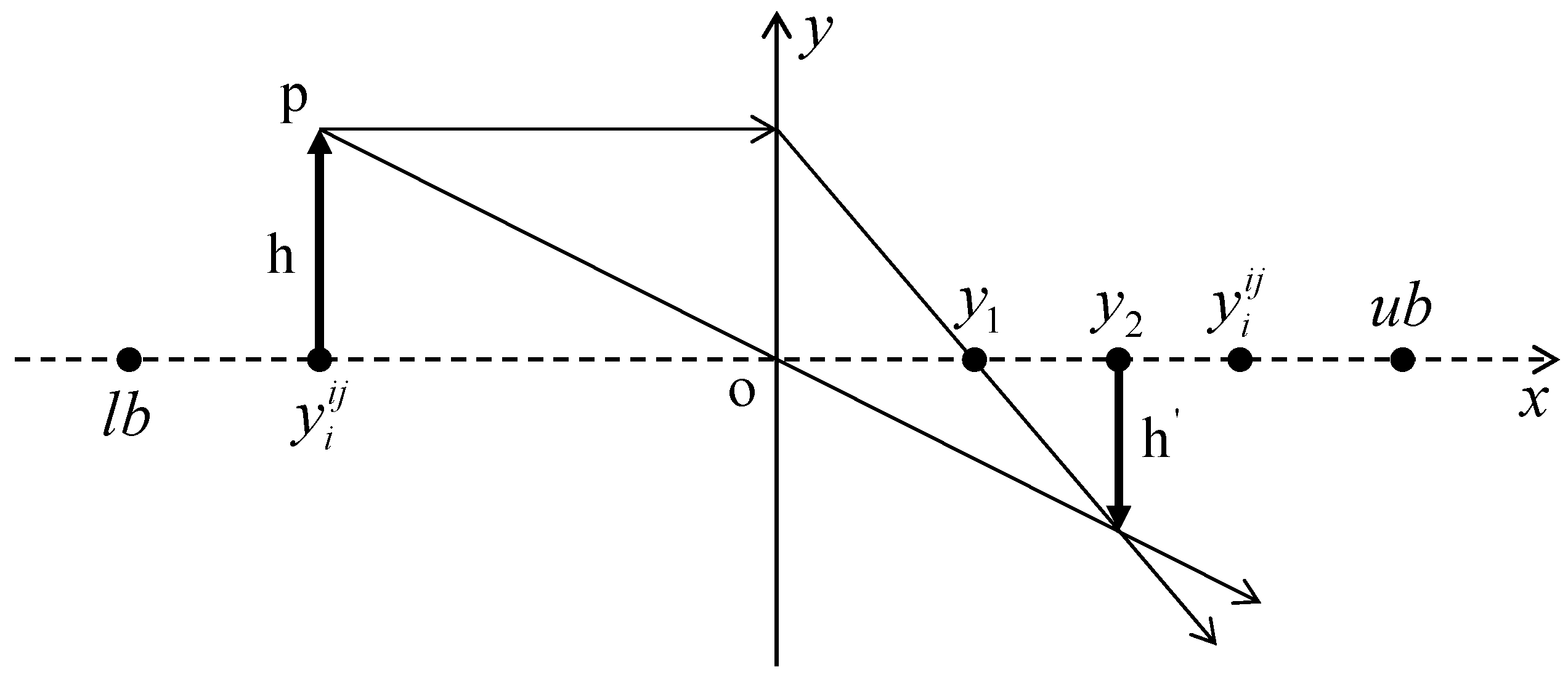
During the preying phase of the BKA, all individuals converge towards the region occupied by the individual with the current optimal fitness value, leading to a reduction in population diversity and a tendency for the algorithm to become trapped in the local optima. To overcome this limitation, this study proposes a reverse learning strategy incorporating dynamic convex lens imaging [53,54]. Through the mechanism of reverse learning, individuals not only follow the position of the current optimal individual but also acquire certain reverse information. This reverse information can be understood as forming a reverse attractive force towards the position of the current optimal individual in the search space. The dynamic aspect is a crucial part of this strategy, as the effect of convex lens imaging adjusts dynamically according to the progress of the search process. This method simulates the dynamic imaging process of a convex lens. During the search process of the algorithm, the movement trajectories of individuals are not only attracted by the current optimal individual but also guided by information from other directions. In this way, the solution set in the search space can be explored more comprehensively, avoiding the dilemma of local optima. The principle of this method is shown in Figure 1.

Figure 1.
Principle of dynamic convex lens imaging-based learning.
In the dynamic lens imaging learning strategy shown in Figure 1, O represents the midpoint of the interval [lb, ub], h denotes the height of the current point P, and h′ represents the height of the image P′ of the light source P. Through the aforementioned principle of dynamic convex lens imaging-based learning, new expression has been derived, as shown in Equation (8).
In the equation: k = 2r, where r has the same meaning as defined previously.
- (3)
- Correction Strategy Based on Fraunhofer Diffraction
Fraunhofer diffraction occurs when the distance between the light source and the observation screen is sufficiently far from the diffraction screen (circular aperture), causing the incident light and the diffracted light to be parallel. In Fraunhofer diffraction, the first dark ring is determined by the first zero of the first-order Bessel function, which occurs approximately at the point given by the following Equation (9):
where a represents the radius of the circular aperture; λ denotes the wavelength of the light source; and θ is the diffraction angle.
Under these conditions, the radius, R, of the diffraction ring can be measured based on the diffraction angle on the screen, yielding the following result:
where L represents the distance from the circular aperture to the screen.
Since θ is typically very small, this study employs the small-angle approximation [55,56] to derive the following Equation (11):
Due to the large variation in the size of random steps in the migration phase of the BKA, slow convergence speed, and the disadvantage of conducting large-scale migration searches even when approaching the global optimal solution, the decision was made to incorporate the Fraunhofer diffraction correction strategy, as shown in Equation (12).
where e, a, and w are constant values used to adjust the size of the leading range of the leader individual.
In summary, the flowchart of the multi-strategy improved Black-winged Kite Algorithm (IBKA) is shown in Figure 2. Step 1: Initialize the population parameters, including the population size N, the maximum number of iterations Max, and the chaotic coefficient r. Generate the initial population using Equation (7), calculate the fitness values of the initial population, and select the individual with the best fitness value as the leader. Step 2: Update the positions of individuals by incorporating the predation process with the reverse learning strategy based on dynamic lens imaging using Equation (8) and the migration process with the Fraunhofer diffraction correction strategy using Equation (12). Step 3: Recalculate the fitness values of the population and reselect the optimal individual as the leader. Step 4: Check if the termination condition is met. If so, end the algorithm; otherwise, repeat Step 2.
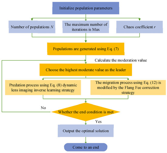
Figure 2.
Flowchart of the multi-strategy improved Black-winged Kite Algorithm.
2.2. Informer
The Informer model introduces three improvements to the Transformer architecture, aiming to enhance computational efficiency and predictive capabilities within the self-attention mechanism [57]. It innovatively incorporates a sparse self-attention mechanism, which reduces the computational complexity of self-attention from quadratic to a more efficient level by streamlining the convolutional pooling operations in the attention layers. Furthermore, the model employs self-attention distillation techniques, effectively reducing the dimensionality and the number of network parameters. This not only strengthens the model’s ability to handle long-term dependencies but also significantly boosts its overall performance. Additionally, the Informer is equipped with an advanced generative decoder that computes all prediction values simultaneously. This feature not only accelerates the prediction process but also ensures a substantial improvement in prediction accuracy, enabling the model to more precisely capture the complex dependencies between inputs and outputs [58,59,60]. The structure of the Informer model is illustrated in Figure 3.
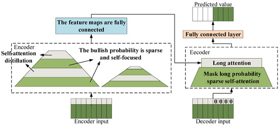
Figure 3.
Structure of the Informer model.
2.3. BiLSTM
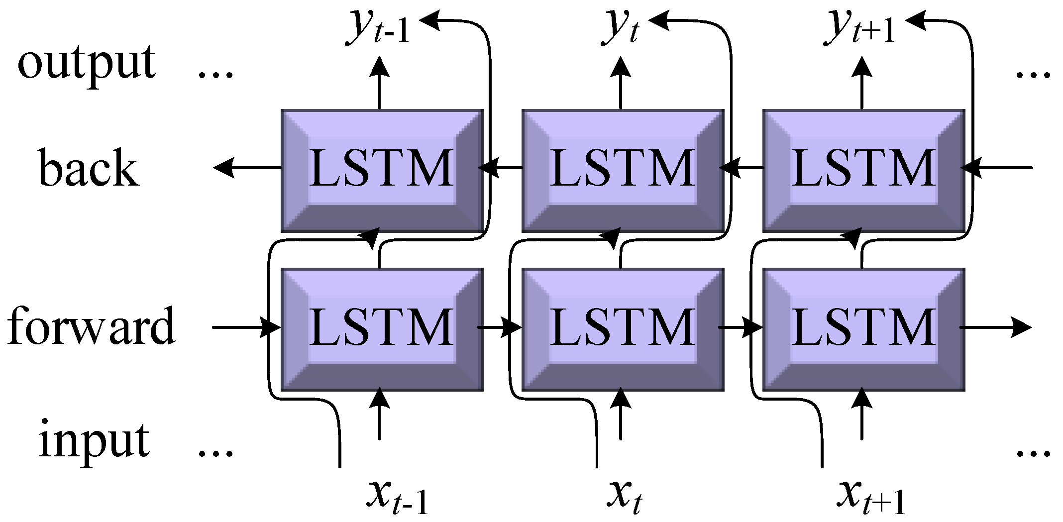
The Bidirectional Long Short-Term Memory (BiLSTM) network model is an improvement upon the traditional Long Short-Term Memory (LSTM) network. BiLSTM integrates two LSTM models, one processing the sequence data in the normal time order and the other processing the same sequence data in the reverse time order [61,62]. Through this bidirectional processing, BiLSTM can simultaneously capture both past and future information in the sequence data, making it more comprehensive than using LSTM alone. The structure of BiLSTM is shown in Figure 4.
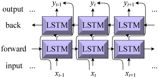
Figure 4.
Bidirectional Long Short-Term Memory (BiLSTM) network.
3. Gas Concentration Prediction Model Based on IBKA-Informer-BiLSTM
3.1. Development of the IBKA-Informer-BiLSTM Gas Concentration Prediction Model
The Informer model excels in processing long time series data, while the BiLSTM model demonstrates outstanding performance in capturing both short-term and long-term dependencies in sequential data. However, BiLSTM’s bidirectional computation increases computational load. In contrast, the Distilling operation in Informer can effectively reduce computational costs. Given these considerations, this study constructs a parallel architecture prediction model by concatenating the outputs of Informer and BiLSTM and fusing features through a fully connected layer. This model combines Informer’s global information extraction capability with BiLSTM’s local temporal relationship modeling ability. Furthermore, the IBKA is employed to optimize the hyperparameters of both models. The specific process is as follows:
- Step 1: The methane data collected from the Buertai Coal Mine is randomly divided into a training set (70%) and a test set (30%), which also serve as the output.
- Step 2: Utilize the temporal nature of the methane data to construct an initial IBKA-Informer-BiLSTM gas prediction model.
- Step 3: Optimize the hyperparameters of the parallel architecture model using the IBKA. The improved algorithm initializes the black-winged kite population through the Tent map, setting parameters such as population size, dimensions, upper and lower limits, and maximum iteration number. The optimization parameters include the hidden dimensions of the parallel architecture model, the number of encoders and decoders, learning rate, and regularization coefficient. During the optimization process, the Root Mean Squared Error (RMSE) is used as the objective function, with criteria including whether the training error is less than 0.01 and whether the maximum iteration number is reached, to ensure the effectiveness of the IBKA.
- Step 4: Construct the final IBKA-Informer-BiLSTM gas prediction model using the optimized parameters and predict the test data to validate the model’s accuracy and applicability. Conduct a comprehensive evaluation of the model’s performance and compare it with other models to demonstrate its predictive accuracy and superiority.
The overall workflow is shown in Figure 5.
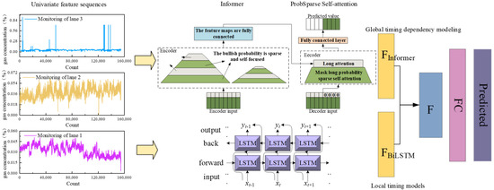
Figure 5.
Workflow of the IBKA-Informer-BiLSTM gas prediction model.
3.2. Project Overview and Data Preprocessing
The Buertai Coal Mine is a super-large mine that is globally pioneering in achieving world-leading levels in three aspects: mine production capacity, main transportation system capacity, and coal washing and processing capabilities. In this mining area, monitoring and predicting methane concentrations are particularly crucial, serving as both an important consideration for environmental protection and a key measure to ensure worker safety and production continuity.
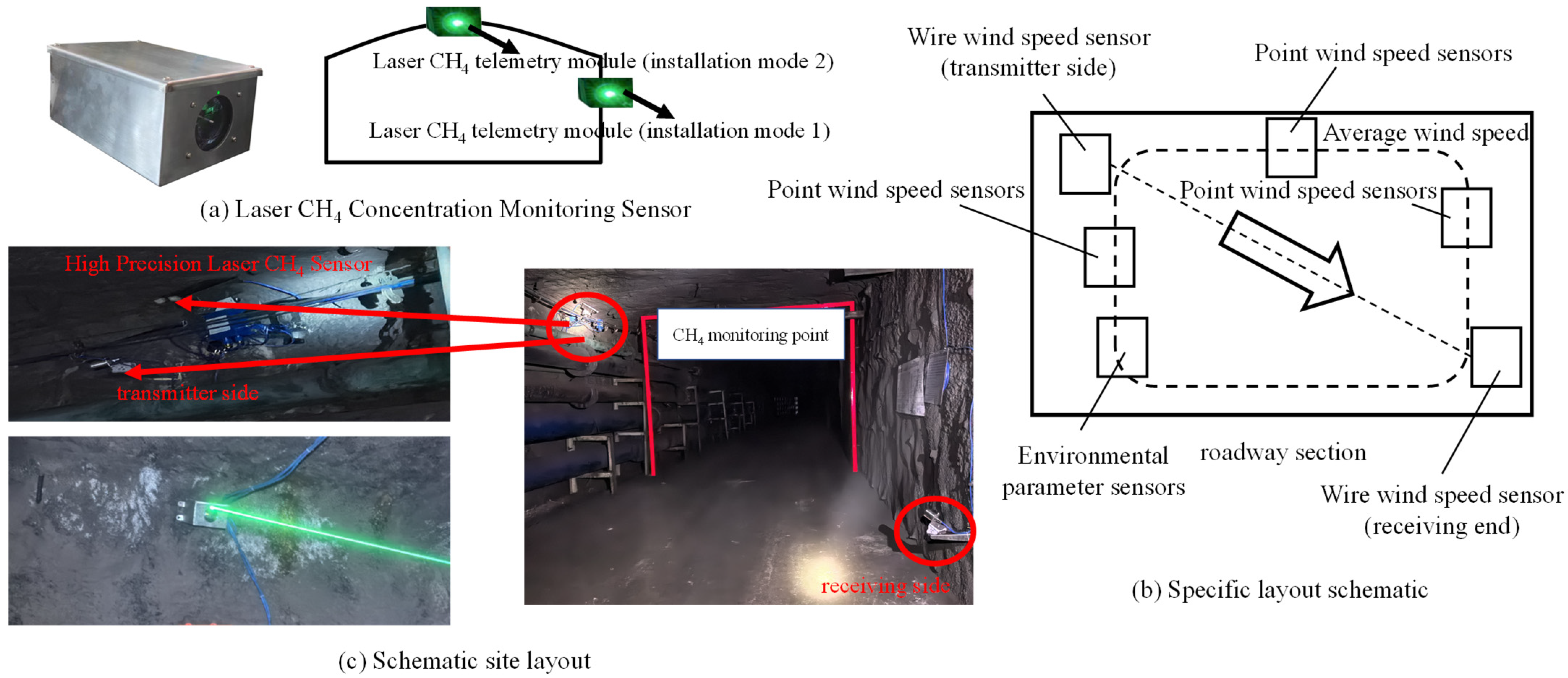
Currently, methane sensors have a detection accuracy of 0.01%, which limits accurate measurements of methane concentrations in the return airflow [63,64]. Therefore, this study employs a laser methane concentration monitoring sensor, as shown in Figure 6a. It can measure the average concentration along a linear path of methane across the entire section. The specific layout scheme is shown in Figure 6b. The linear arrangement of sensors enables continuous measurements along the path, making it suitable for large-scale applications in complex environments and outperforming point sensors. The monitoring process is depicted in Figure 6c. Monitoring points are set up at the 1400 m mark of the return airway in the third panel of the 12th coal seam, the 1500 m mark of the main return airway of the 12th coal seam, and the 460 m mark of the return airway in the second panel of the 42nd coal seam in the Buertai Coal Mine. The monitoring activity will be conducted from 1 April 2024, to 31 July 2024, with data recorded every 60 s.
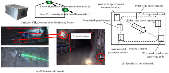
Figure 6.
Schematic layout of the laser methane concentration monitoring sensor.
The selected monitoring points are located in the roadways with rectangular sec-tions, with large ventilation section dimensions to meet the demand for efficient ventilation: the section dimensions of the 12-coal three-panel area return alley (1400 m) and the 12-coal general return alley (1500 m) are 6.0 m × 4.0 m (width × height), and the section dimensions of the 42-coal two-panel area return alley (460 m) are 5.5 m × 3.8 m (width × height). According to the design of the ventilation system and measurement data of the Bultai Mine, the range of wind speeds in the tunnel at the selected monitoring point is as follows: minimum wind speed: 1.2 m/s, maximum wind speed: 4.8 m/s. The wind speeds at the selected monitoring point are as follows: minimum wind speed: 1.2 m/s, maximum wind speed: 4.8 m/s. The above wind speed range ensures the effectiveness of air flow and also provides dynamic conditions for methane concentration distribution monitoring. The laser methane concentration monitoring sensors are deployed in the above sections and paths, which can capture the changes in methane concentration in the sections under the complex environment and provide high-precision real-time monitoring data.
To ensure that the model can efficiently utilize the limited field measurement data for adequate learning, this study recognizes the presence of outliers in different datasets. Therefore, strict data preprocessing steps have been implemented across all datasets, with a focus on screening and eliminating these outliers. The aim is to safeguard the model from the interference of abnormal data during both the training and prediction stages, thereby enhancing its accuracy and reliability.
3.3. Superiority Verification and Hyperparameter Optimization of IBKA
3.3.1. Testing and Comparative Analysis of Optimization Algorithms
Benchmark Test Functions
To verify the effectiveness and robustness of the algorithm proposed in this study for solving optimization problems, 50 independent experiments were conducted on 12 typical benchmark functions. The best values (Best), mean values (Mean), and standard deviations (Std) of the obtained optimal solutions were calculated to reflect the algorithm’s upper gradient limit for optimization, overall performance, and stability. The unimodal functions F1, F4, F6, F8, F9, and F10, as well as the multimodal functions F2, F3, F5, F7, F11, and F12, exhibit different morphological characteristics. Unimodal functions are characterized by typically having only one strict optimal solution within the search interval, tending to test the algorithm’s search capability and convergence speed. Multimodal functions, on the other hand, are characterized by multiple local extrema within the search interval, tending to test the algorithm’s ability to identify local optima and expand the search scope for global exploration. The specific benchmark functions are shown in Table 1.

Table 1.
Benchmark test functions.
Selection of Key Parameters for the Improved Algorithm
Among the key parameters of the IBKA, the population size, N, is set to 100, the maximum number of iterations Max is 1000, and the probability value p is 0.9. Additionally, the parameters e and w in the Fraunhofer diffraction correction strategy directly influence the movement of individual positions in the population, affecting the exploration accuracy and convergence speed of the optimal solution. To determine the optimal parameter combination, experiments were conducted separately, where e was set to 0.6, 0.7, 0.8, and 0.9, and w was set to 2, 3, 4, and 5. Detailed records were kept for each test function and its corresponding parameter settings. Subsequently, the results obtained by each set of parameters for a specific test function were compared with the optimal results, and the ratios were calculated and log-transformed to quantitatively assess the specific impact of different parameter configurations on the optimization performance of the IBKA. All detailed experimental results are shown in Table 2.
Table 2.
Impact of different parameters on the optimization performance of the IBKA.
For the same function, results closer to 0 indicate that the corresponding parameters are more optimal among the 16 test functions. (I) When e = 0.6 and w = 3, the best performance was achieved for the functions F3, F6, F7, and F8. (II) When e = 0.9 and w = 3, the best performance was achieved for the functions F2 and F9. (III) When e = 0.6 and w = 4, the best performance was achieved for the functions F1, F6, and F10. When other parameter values were used, the overall performance of the remaining parameter combinations did not reach the level of the three parameter combinations discussed earlier for solving these 12 test functions. Therefore, the analysis in this study focused on these three parameter configurations: I, II, and III. Based on the analysis in Table 2, it can be seen that the IBKA performed best overall across the 12 test functions when e = 0.6 and w = 3, compared to the other two scenarios. Based on these analyses, this study selects e = 0.6 and w = 3 as the parameters for the IBKA.
Ablation Experiment
The BKA initialized with the Tent chaotic map population is named BKA1, the BKA incorporating the dynamic lens imaging strategy for the predation process is named BKA2, and the BKA incorporating the Fraunhofer diffraction correction strategy for the migration process is named BKA3. Twenty independent experiments were conducted for each set of parameters. The statistical results are shown in Table 3.
Table 3.
Comparison of different improvement strategies.
Based on the analysis of Table 3, the IBKA outperforms the singly improved BKA strategies and the basic BKA in functions F2 to F5 and F8. In F5 and F7, BKA2 achieves the same optimization accuracy as the IBKA. In F4 and F8, both BKA2 and BKA3 are close to the optimal values obtained by the IBKA. Across all test functions, the improved BKA2 outperforms BKA1. Overall, the IBKA performs the best. The IBKA with three improvement strategies demonstrates significantly better optimization accuracy and robustness compared to the singly improved algorithms, effectively compensating for the limitations of a single strategy and maximizing the performance of the basic BKA.
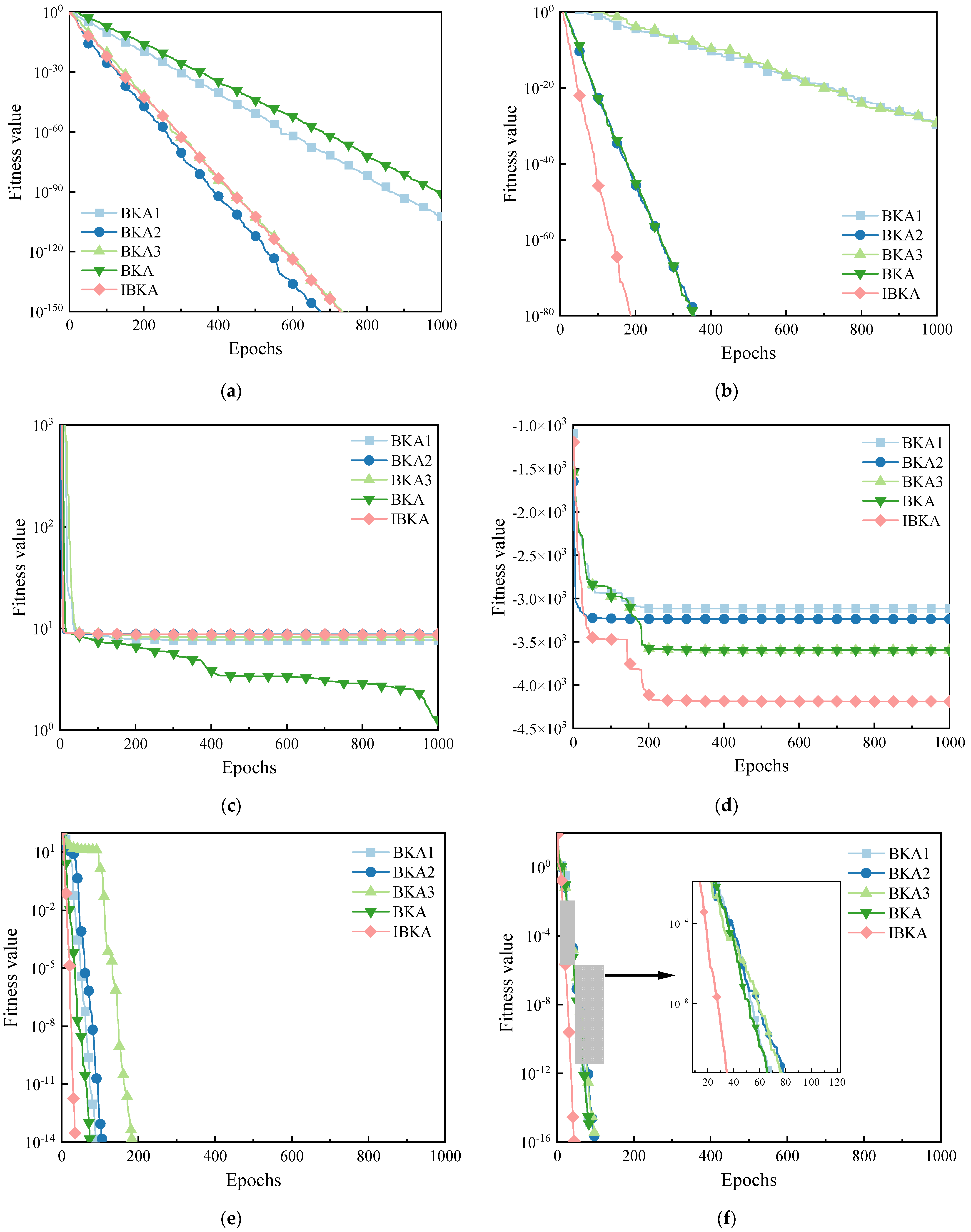
To further analyze the performance of the algorithms, the average convergence curves of the improved algorithms for some test functions are plotted, as shown in Figure 7. Within the limited number of iterations in Figure 7a,b, the corresponding curves of BKA1, BKA2, BKA3, BKA, and IBKA converge in sequence. In Figure 7a, the improved algorithms all outperform the BKA with significantly faster convergence speeds, among which BKA2 is the best, and IBKA and BKA3 are close behind as the second-best algorithms. In Figure 7b, the IBKA demonstrates significantly better convergence speed and accuracy than the other algorithms. In Figure 7c, the algorithms do not converge, and the convergence curves of each algorithm follow a similar trend. In the early stages, when all algorithms are trapped in local optima, BKA2 has the steepest convergence curve, followed by the IBKA. Eventually, all algorithms become trapped in the local optima, but the BKA shows a tendency to escape from the local optima. In Figure 7d, the IBKA shows a tendency to escape from local optima when one-fifth of the iteration process is completed. During the first one-fifth of the iteration process, the IBKA consistently converges with a steep slope and is the closest to the optimal solution among all algorithms. In Figure 7e,f, all algorithms converge. In Figure 7e, BKA1, BKA2, BKA, and IBKA follow similar trends and converge with steep slopes in the early stages. Among them, the IBKA has the steepest slope. When one-tenth of the iteration process is completed, BKA3 shows a tendency to fall into a local optimum, but it quickly escapes after a short period of iteration. In Figure 7f, all algorithms converge with steep slopes and follow similar trends, with the IBKA consistently leading the other algorithms in convergence slope. It can be seen that the incorporation of the Tent chaotic map, the dynamic lens imaging reverse learning strategy, and the Fraunhofer diffraction correction strategy increases the population diversity of individuals and effectively improves performance. These improvements help overcome the algorithm’s deficiencies when dealing with single-peak and multi-peak functions.
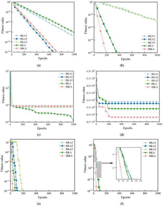
Figure 7.
Average Convergence Curves of different improved algorithms. Average Convergence Curve of (a) F2, (b) F3, (c) F5, (d) F8, (e) F9, (f) F11.
Validation Line for the Superiority of the IBKA
To comprehensively validate the superiority of the IBKA, this study conducted an in-depth comparison with several classic and recent intelligent optimization algorithms. These algorithms include the classic Particle Swarm Optimization (PSO), Sparrow Search Algorithm (SSA), Whale Optimization Algorithm (WOA), Grey Wolf Optimizer (GWO), as well as the recently proposed Sand Cat Swarm Optimization (SCSO) and Sailfish Optimizer (SFO) [65]. The test function results, algorithm parameter selections, and evaluation metrics for this comparison all follow the stipulations outlined in Section 3.1 to ensure fairness and accuracy in the comparison. For PSO, C1 and C2 are set to 1.5, and w linearly decreases from 0.9 to 0.4. For SSA, PNum and SNum are set to 0.2 times the population size N, and R2 is set to 0.8. The specific parameter settings for the other algorithms are based on the relevant literature [66,67,68]. The experimental results are shown in Table 4.
Table 4.
Comparison of optimization results among various algorithms.
Based on the analysis of Table 4, it can be observed that due to the different optimization mechanisms employed by each algorithm, there are variations in their search accuracy and performance. When comparing the algorithms with a search dimension of 10 for all benchmark test functions, the IBKA demonstrates the best overall performance, followed by SFO, SSA, SCSO, GWO, and PSO showing the weakest performance. In cases where the solution accuracy of each algorithm for F1, F2, F4, F6–F9, F11, and F12 is relatively low, the IBKA is able to maintain an average value equal to the theoretical value with a standard deviation of 0. For the remaining test functions, the solution accuracy of the IBKA is more than 10 orders of magnitude higher than that of the SFO algorithm. In summary, the IBKA exhibits high accuracy, good stability, and superior performance in solving test functions, outperforming algorithms such as SFO and the SSA.
Wilcoxon Rank-Sum Test
To validate whether the results of each run of the proposed skill algorithm in this study are statistically significantly different from those of other algorithms, the Wilcoxon Rank-Sum Test was conducted at a significance level of 5% [69,70]. Table 5 presents the p-values obtained through the Wilcoxon Rank-Sum Test when comparing the IBKA with the SSA, SCSO, and SFO during the execution of 12 benchmark test functions. A p-value less than 0.05 is considered a strong indication to reject the null hypothesis. The NA values indicate that significance could not be determined for the corresponding algorithm in the rank-sum test. In Table 5, the p-values for the comparisons between the IBKA and the SSA, SCSO, and SFO are denoted as P1, P2, and P3, respectively.
Table 5.
p-values of Wilcoxon Rank-Sum Test for test functions.
Based on the analysis of Table 5, the majority of the p-values for the IBKA are less than 0.05, indicating that the algorithm’s performance is statistically significant. This demonstrates that the IBKA has better convergence accuracy than the other algorithms, further proving the effectiveness of the improved algorithm proposed in this study.
3.3.2. Hyperparameter Optimization Based on the IBKA
In this study, the IBKA was employed to optimize seven hyperparameters of the Informer model, including the hidden layer dimension (d_model), the number of attention heads (n_heads), the number of encoder and decoder layers (e_layers), as well as the hidden layer units (units), regularization coefficient (L2), and learning rate (learning_rate) of the BiLSTM model. The initial learning rate is crucial for gradient descent, influencing the convergence speed and the ability to reach a local minimum. A learning rate that is too low results in slow convergence, while a rate that is too high may prevent convergence altogether. Increasing the hidden layer dimension of the Informer enhances its expressive capability but also raises the risk of overfitting. A higher number of attention heads facilitates the capture of temporal features from multiple perspectives but increases computational complexity. More encoder layers enrich the feature representation, benefiting complex temporal dependencies, while additional decoder layers improve the quality of sequence generation. A greater number of BiLSTM units enhances learning capacity but also increases the risk of overfitting. The regularization coefficient is used to balance complexity and generalization ability, controlling model complexity and reducing the risk of overfitting.
By inputting the preprocessed data samples into the constructed parallel architecture model and leveraging the excellent optimization and convergence speed of the IBKA, optimized hyperparameters can be obtained. Table 6 presents the random initialization ranges and optimal values for the IBKA parameter optimization.
Table 6.
Random initialization ranges and optimal values of hyperparameters.
4. Model Evaluation and Comparison
4.1. Model Training and Testing
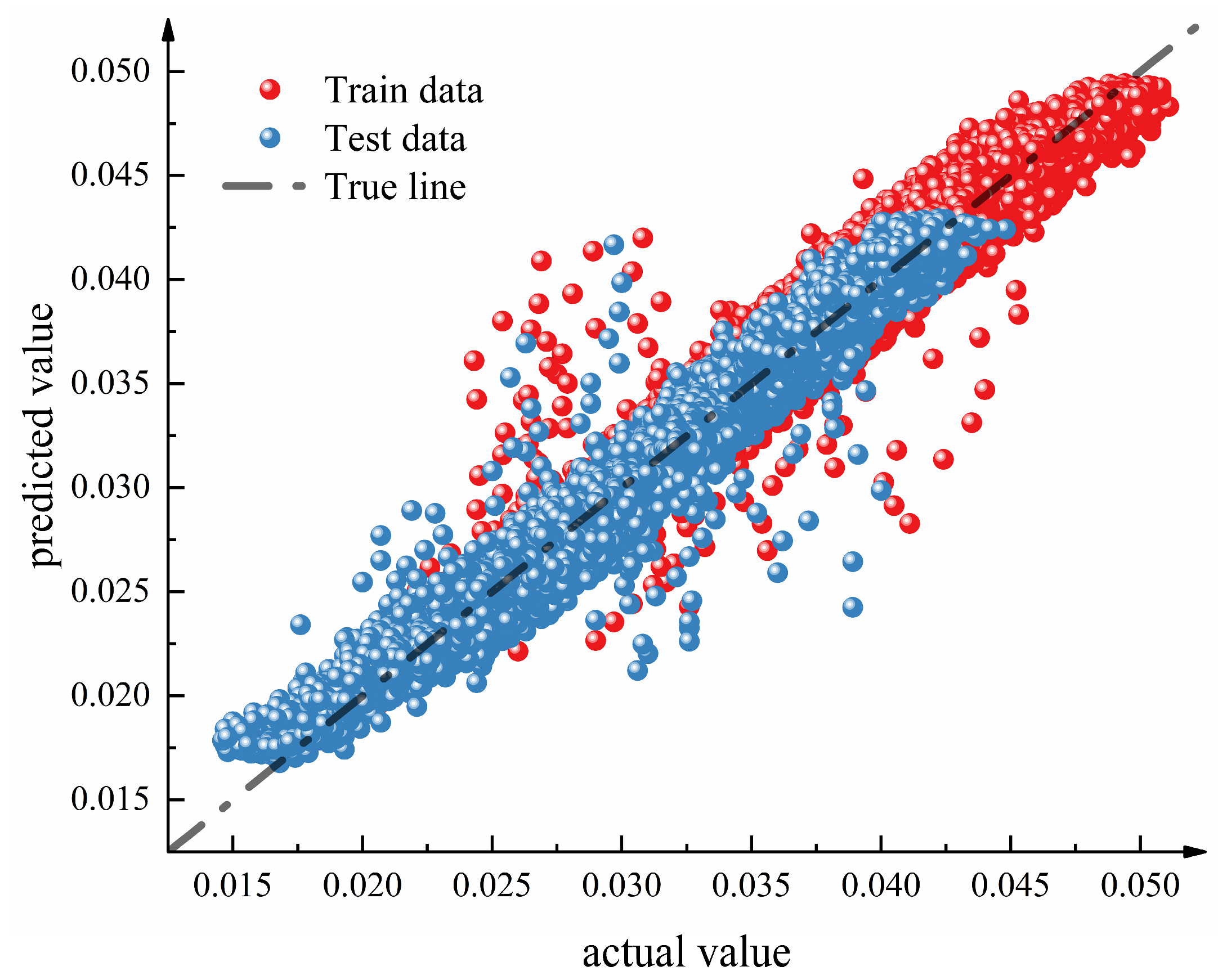
In this study, to evaluate the generalization capability of the model on new data, the gas dataset was randomly split into a training set and a test set in a 7:3 ratio. Figure 8 presents the prediction results of the model on both the training and test sets. The analysis of Figure 8 reveals that the distribution of prediction results for both the training and test sets closely follows a straight line, indicating that the IBKA-Informer-BiLSTM gas prediction model exhibits stable and accurate prediction performance on both sets, which is close to the true values. This demonstrates the good feasibility and applicability of the model in practical applications.
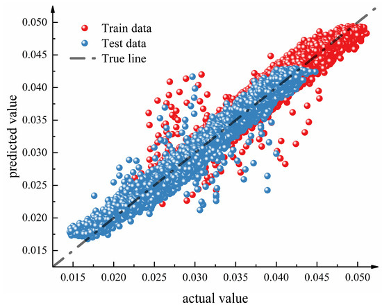
Figure 8.
Prediction results of the model on the training and test sets.
4.2. Model Comparison
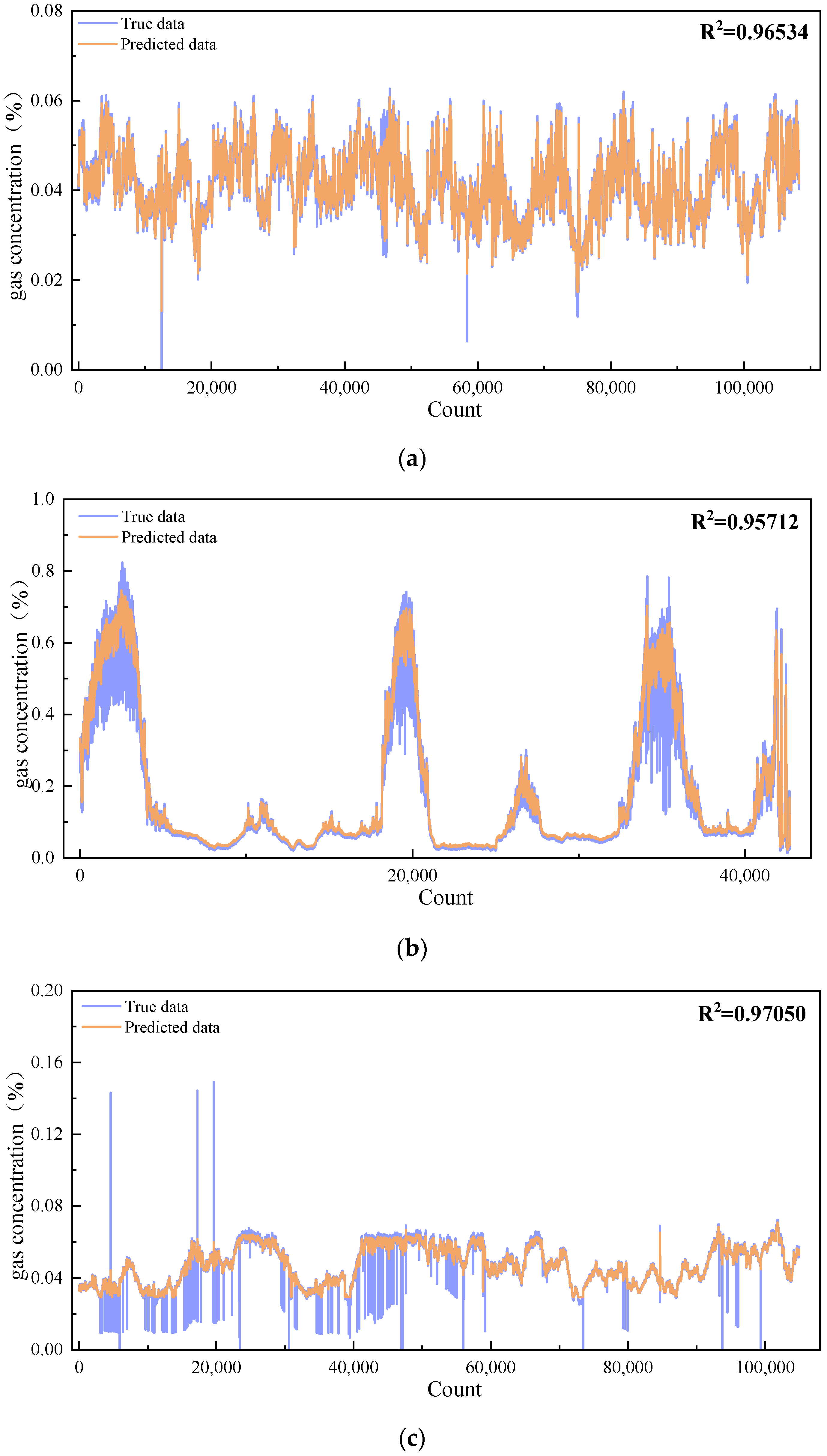
To validate the superiority of the proposed IBKA-Informer-BiLSTM prediction model, this study conducted comparative experiments with seven other models, specifically LSTM-Informer, LSTM, BiLSTM, Informer, Autoformer, XGBoost, and LR. Given the characteristics of the hyperparameters used in these models, the IBKA was again employed to effectively explore the hyperparameter space. The names of the hyperparameters and their corresponding optimal values are shown in Table 7. Additionally, four commonly used statistical metrics were adopted to measure the goodness of fit between the predicted and actual values, including Mean Absolute Error (MAE), Mean Absolute Percentage Error (MAPE), Root Mean Squared Error (RMSE), and the coefficient of determination R2. Their mathematical expressions are shown in Equations (13)–(16). The evaluation results for each model are shown in Table 8.
Table 7.
Hyperparameters for each model.
Table 8.
Evaluation metrics results for each model.
Based on the analysis of Table 8, the IBKA-Informer-LSTM model demonstrates impressive performance in predicting methane concentrations using the dataset collected from a high-precision methane sensor located 1400 m into the return airway of the third panel in the No. 12 coal seam at Buertai Mine. The model achieves MAE values of 0.00067624 and 0.0005971 on the training and test sets, respectively, with RMSE values of 0.00088187 and 0.0008005. Furthermore, the R2 values on the training and test sets are 0.9769 and 0.9589, respectively. Therefore, the IBKA-Informer-LSTM model outperforms the other models in this study.
4.3. Verification of Model Generalization Capability
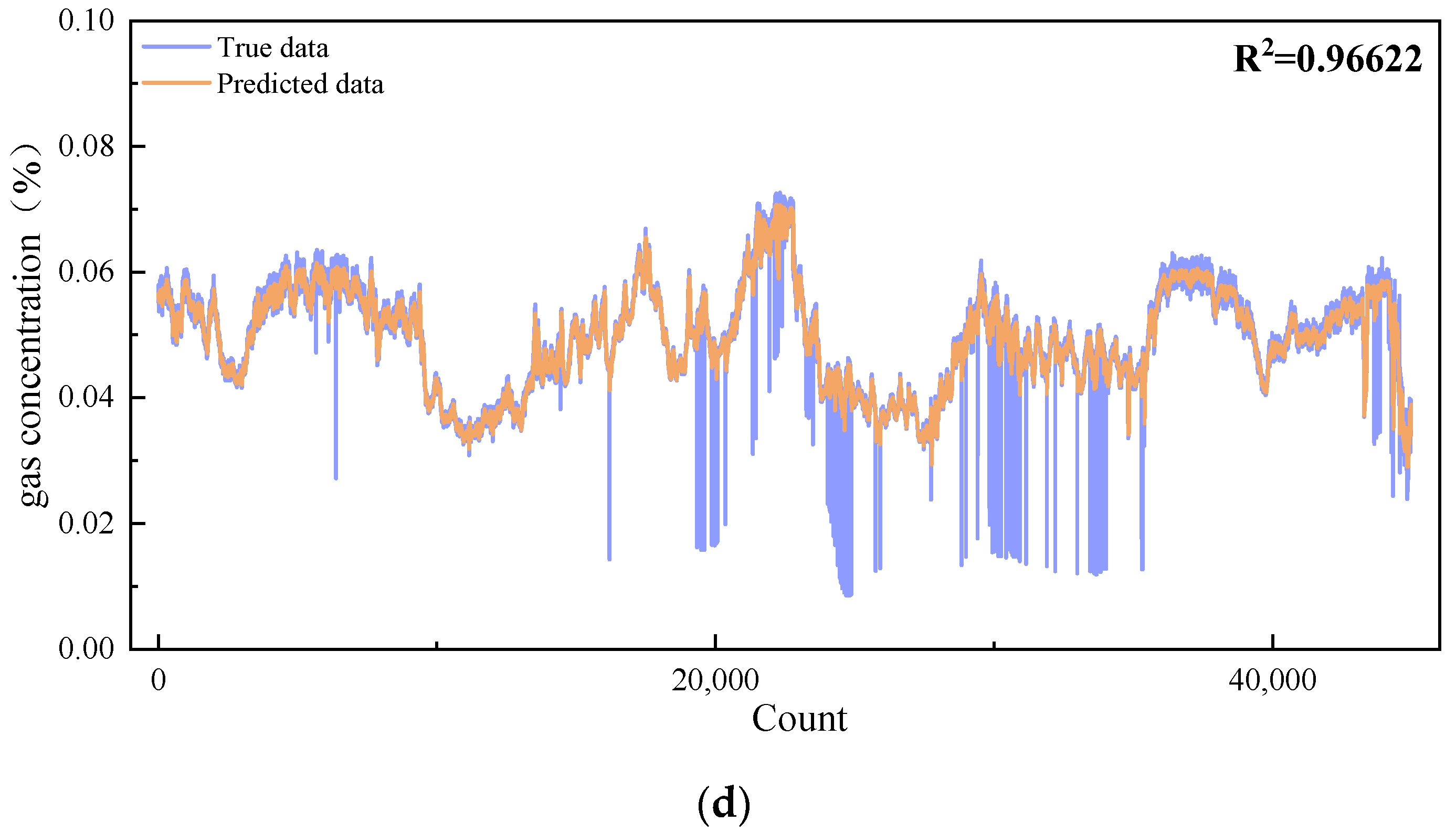
The generalization capability of the model developed in this study was validated using two datasets collected by laser methane concentration monitoring sensors located 1500 m into the main return airway of the No. 12 coal seam and 460 m into the return airway of the second panel in the No. 42 coal seam at Buertai Mine. The model parameters and optimization methods were consistent with those described previously. The fitting results for the training and test sets are shown in Figure 9.
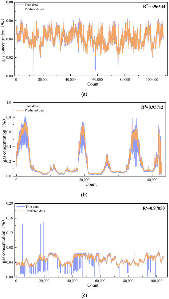
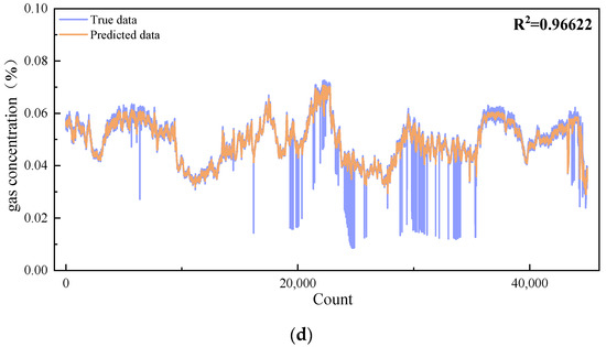
Figure 9.
Fitting results for datasets from other roadways. (a) Fitting effect of the training set for methane concentration at 1500 m into the main return airway of the No. 12 coal seam. (b) Fitting Effect of the test set for methane concentration at 1500 m into the main return airway of the No. 12 coal seam. (c) fitting effect of the training set for methane concentration at 460 m into the return airway of the second panel in the No. 42 coal seam. (d) Fitting results of the test set for methane concentration at 460 m into the return airway of the second panel in the No. 42 coal seam.
As shown in Figure 9, the IBKA-Informer-LSTM model for predicting methane concentrations in coal mine roadways, developed in this study, demonstrates superior performance across different datasets within the same application scenario and model environment. The R2 values on both the training and test sets exceed 0.95, indicating exceptional prediction accuracy. Additionally, the values for MAPE, MAE, and RMSE are notably low, further attesting to the model’s potential for methane prediction in various coal mine roadways. This research enhances the preventive capabilities for coal mine roadway safety. As can be seen in Figure 9, the maximum concentration of gas in the roadway is 0.16%, which is significantly lower than the lower limit of gas explosion concentration (5%). This result verifies the safety of the selected tunnel in terms of gas concentration control from the side, strongly indicates the effectiveness of the current ventilation and gas management measures and provides data support for the safety of production operations. Therefore, the findings of this study not only hold significant theoretical importance but also exhibit substantial practical value, providing new methods and insights for coal mine roadway safety.
5. Discussions
This study introduces a methane concentration prediction model for coal mine roadways based on an Improved Black Kite Algorithm (IBKA) coupled with Informer-BiLSTM, demonstrating superior predictive accuracy and generalization ability. The proposed enhancements to the Black Kite Algorithm, including Tent chaotic mapping and Fraunhofer diffraction search strategies, effectively improve its search efficiency and convergence speed. Coupled with the optimization of Informer-BiLSTM hyperparameters, the model achieves robust performance, as evidenced by R2 values exceeding 0.95 in both training and test datasets. These findings underscore the practical applicability and reliability of the IBKA-Informer-BiLSTM model in real-world methane concentration monitoring.
However, a limitation of the current approach is the lack of cross-validation techniques to assess model stability. While the study clearly outlines the delineation of the training and test datasets and achieved impressive metrics, cross-validation would provide a more comprehensive assessment of model robustness and parameter stability. Incorporating cross-validation would further confirm the consistency of the predictions and ensure the reliability of the model under different conditions. Future work will explore the application of cross-validation in optimizing and validating model performance. In addition, extending the application of the model to other coal mines with different geological conditions could further assess its adaptability and effectiveness in enhancing safety measures in mining operations.
6. Conclusions
In this study, a novel prediction architecture, namely the IBKA-Informer-BiLSTM model, was designed. The IBKA component in this model was optimized through the integration of the Tent chaotic mapping technique, dynamic convex lens imaging learning mechanism, and Fraunhofer diffraction search algorithm. Subsequently, the IBKA was fused with the Informer-BiLSTM model, and a meticulous tuning process was conducted for seven key hyperparameters, including the number of hidden layers, learning rate, and regularization coefficient. In terms of data processing, the methane concentration dataset from Buertai Mine’s roadways was randomly split into a training set (70%) and a test set (30%). Based on this partition, the IBKA-Informer-BiLSTM model for predicting methane concentrations in coal mine roadways was constructed. To comprehensively evaluate its prediction performance, a comparative analysis was conducted with six mainstream models. Furthermore, to further verify its generalization ability, two additional methane concentration datasets from Buertai Mine were used for testing. The research conclusions are as follows:
- (1)
- By improving the traditional Black-winged Kite Algorithm (BKA), including the introduction of Tent chaotic mapping, the integration of dynamic convex lens imaging, and the adoption of Fraunhofer diffraction search strategy, the experimental results demonstrated that the performance of the IBKA was significantly enhanced, exhibiting higher search accuracy, faster convergence speed, and robust practicality.
- (2)
- The combination of the IBKA with the Informer-BiLSTM prediction model, through the optimization of seven hyperparameters within the model, further improved the prediction accuracy. The research results indicated that this coupled model achieved low MAE, MAPE, and RMSE values, along with a high R2 value, on both the training and test sets, showcasing excellent prediction performance.
- (3)
- A comparative analysis was conducted between the prediction results of the IBKA-Informer-BiLSTM model and six reference models. The results revealed that the coupled model achieved an MAE of 0.0005971, an RMSE of 0.0008005, and an R2 of 0.9589 on the test set. This conclusion demonstrates the superiority of the IBKA-Informer-BiLSTM model in predicting methane concentrations in coal mine roadways.
- (4)
- The application of the model to other methane concentration datasets from Buertai Mine’s roadways resulted in R2 values exceeding 0.95 on both the training and test sets, validating the generalization ability of the IBKA-Informer-BiLSTM prediction model.
Author Contributions
H.Q.: Conceptualization, Supervision, Writing—review and editing. X.S.: Writing—original draft, Investigation, Methodology. H.G.: Formal analysis, Investigation, Supervision. Q.C.: Methodology. J.G.: Validation. C.L.: Investigation. All authors have read and agreed to the published version of the manuscript.
Funding
This study is supported by the National Key Research and Development Program of China (Grant No. 2020YFA0711802), the National Natural Science Foundation of China (Grant No. 52074283) the National Key Research and Development Program of China (Grant No. 2023YFC3009100),and the China University of Mining and Technology: Enhancing Independent Innovation Capability through “Double First-class” Construction of Safety Discipline Group (Grant No. 2022ZZCX-AQ06). The authors are very grateful for the above support.
Data Availability Statement
The original contributions presented in this study are included in the article. Further inquiries can be directed to the corresponding author.
Conflicts of Interest
The authors declare no conflict of interest.
References
- Wang, Y.; Fu, G.; Lyu, Q.; Jingru, W.; Yali, W.; Meng, H.; Yuxuan, L.; Xuecai, X. Accident case-driven study on the causal modeling and prevention strategies of coal-mine gas-explosion accidents: A systematic analysis of coal-mine accidents in China. Resour. Policy 2024, 88, 104425. [Google Scholar] [CrossRef]
- Zhang, J.; Xu, K.; Reniers, G.; You, G. Statistical analysis the characteristics of extraordinarily severe coal mine accidents (ESCMAs) in China from 1950 to 2018. Process Saf. Environ. Prot. 2020, 133, 332–340. [Google Scholar] [CrossRef]
- Xie, X.; Shen, S.; Fu, G.; Xueming, S.; Jun, H.; Qingsong, J.; Zhao, S. Accident case data–accident cause model hybrid-driven coal and gas outburst accident analysis: Evidence from 84 accidents in China during 2008–2018. Process Saf. Environ. Prot. 2022, 164, 67–90. [Google Scholar] [CrossRef]
- Ray, S.K.; Khan, A.M.; Mohalik, N.K.; Mishra, D.; Mandal, S.; Pandey, J.K. Review of preventive and constructive measures for coal mine explosions: An Indian perspective. Int. J. Min. Sci. Technol. 2022, 32, 471–485. [Google Scholar] [CrossRef]
- Bondarenko, A.V.; Islamov, S.R.; Ignatyev, K.V.; Mardashov, D.V. Laboratory studies of polymer compositions for well-kill under increased fracturing. Perm J. Pet. Min. Eng. 2020, 20, 37–48. [Google Scholar] [CrossRef] [PubMed]
- Legkokonets, V.A.; Islamov, S.R.; Mardashov, D.V. Multifactor analysis of well killing operations on oil and gas condensate field with a fractured reservoir. In Topical Issues of Rational Use of Mineral Resources, Proceedings of the International Forum-Contest of Young Researchers, Petersburg, Russia, 18–20 April 2018; CRC Press: Boca Raton, FL, USA, 2019; pp. 111–118. [Google Scholar]
- Liu, J.; Wang, S.; Wei, N.; Chen, X.; Xie, H.; Wang, J. Natural gas consumption forecasting: A discussion on forecasting history and future challenges. J. Nat. Gas Sci. Eng. 2021, 90, 103930. [Google Scholar] [CrossRef]
- Zou, Q.; Liu, H.; Jiang, Z.; Wu, X. Gas flow laws in coal subjected to hydraulic slotting and a prediction model for its permeability-enhancing effect. Energy Sources Part A Recovery Util. Environ. Eff. 2021, 1–15. [Google Scholar] [CrossRef]
- Liu, A.; Liu, S.; Wang, G.; Elsworth, D. Predicting fugitive gas emissions from gob-to-face in longwall coal mines: Coupled analytical and numerical modeling. Int. J. Heat Mass. Transf. 2020, 150, 119392. [Google Scholar] [CrossRef]
- Ma, W.; Ji, X.; Ding, L.; Yang, S.X.; Guo, K.; Li, Q. Automatic Monitoring Methods for Greenhouse and Hazardous Gases Emitted from Ruminant Production Systems: A Review. Sensors 2024, 24, 4423. [Google Scholar] [CrossRef] [PubMed]
- Jahan, I.; Mehana, M.; Matheou, G.; Viswanathan, H. Deep Learning-Based quantifications of methane emissions with field applications. Int. J. Appl. Earth Obs. Geoinf. 2024, 132, 104018. [Google Scholar] [CrossRef]
- Iwaszenko, S.; Kalisz, P.; Słota, M.; Rudzki, A. Detection of natural gas leakages using a laser-based methane sensor and UAV. Remote Sens. 2021, 13, 510. [Google Scholar] [CrossRef]
- Zhang, S.; Ma, J.; Zhang, X.; Guo, C. Atmospheric remote sensing for anthropogenic methane emissions: Applications and research opportunities. Sci. Total Environ. 2023, 893, 164701. [Google Scholar] [CrossRef] [PubMed]
- Zhang, G.; Wang, E. Risk identification for coal and gas outburst in underground coal mines: A critical review and future directions. Gas Sci. Eng. 2023, 118, 205106. [Google Scholar] [CrossRef]
- Anani, A.; Adewuyi, S.O.; Risso, N.; Nyaaba, W. Advancements in machine learning techniques for coal and gas outburst prediction in underground mines. Int. J. Coal Geol. 2024, 285, 104471. [Google Scholar] [CrossRef]
- Wen, H.; Yan, L.; Jin, Y.; Wang, Z.; Guo, J.; Deng, J. Coalbed methane concentration prediction and early-warning in fully mechanized mining face based on deep learning. Energy 2023, 264, 126208. [Google Scholar] [CrossRef]
- Nie, Z.; Ma, H.; Zhang, Y. Research on Gaussian Plume Model of Gas Diffusion in Coal Mine Roadway Based on BP Neural Network Optimized by Genetic Algorithm. IOP Conf. Ser. Earth Environ. Sci. 2020, 526, 012158. [Google Scholar] [CrossRef]
- Guo, R.; Xu, G. Research on coal mine gas concentration multi-sensor prediction model based on information fusion and GA-SVM. China Saf. Sci. J. 2013, 23, 34–38. [Google Scholar]
- Luo, Z.; Zhai, H.; Tong, J. Incorporating multi-features and XGBoost algorithm for gas concentration prediction. China Min. Mag. 2024, 33 (Suppl. S1), 359–363, 370. [Google Scholar] [CrossRef]
- Fu, H.; Liu, Y.Z.; Xu, N.; Zhang, J.N. Research on gas concentration prediction based on multi-sensor-deep long short-term memory network fusion. Chin. J. Sens. Actuators 2021, 34, 784–790. [Google Scholar]
- Li, W.; Wang, G.G.; Gandomi, A.H. A survey of learning-based intelligent optimization algorithms. Arch. Comput. Methods Eng. 2021, 28, 3781–3799. [Google Scholar] [CrossRef]
- Tao, F.; Zhang, L.; Laili, Y. Configurable Intelligent Optimization Algorithm; Springer: Berlin/Heidelberg, Germany, 2015. [Google Scholar]
- Su, Z.; Wang, J.; Lu, H.; Zhao, G. A new hybrid model optimized by an intelligent optimization algorithm for wind speed forecasting. Energy Convers. Manag. 2014, 85, 443–452. [Google Scholar] [CrossRef]
- Cheng, S.; Qin, Q.; Chen, J.; Zhao, G. Brain storm optimization algorithm: A review. Artif. Intell. Rev. 2016, 46, 445–458. [Google Scholar] [CrossRef]
- Gad, A.G. Particle swarm optimization algorithm and its applications: A systematic review. Arch. Comput. Methods Eng. 2022, 29, 2531–2561. [Google Scholar] [CrossRef]
- Müller, A.J.; Michell, R.M.; Pérez, R.A.; Lorenzo, A.T. Successive Self-nucleation and Annealing (SSA): Correct design of thermal protocol and applications. Eur. Polym. J. 2015, 65, 132–154. [Google Scholar] [CrossRef]
- Khalid, O.W.; Isa, N.A.M.; Sakim, H.A.M. Emperor penguin optimizer: A comprehensive review based on state-of-the-art meta-heuristic algorithms. Alex. Eng. J. 2023, 63, 487–526. [Google Scholar] [CrossRef]
- Qiao, L.; Liu, K.; Xue, Y.; Tang, W.; Salehnia, T. A multi-level thresholding image segmentation method using hybrid Arithmetic Optimization and Harris Hawks Optimizer algorithms. Expert Syst. Appl. 2024, 241, 122316. [Google Scholar] [CrossRef]
- Zhang, Y.; Mo, Y. Chaotic adaptive sailfish optimizer with genetic characteristics for global optimization. J. Supercomput. 2022, 78, 10950–10996. [Google Scholar] [CrossRef]
- Niu, P.; Niu, S.; Chang, L. The defect of the Grey Wolf optimization algorithm and its verification method. Knowl.-Based Syst. 2019, 171, 37–43. [Google Scholar] [CrossRef]
- Wang, J.; Wang, W.; Hu, X.; Qiu, L.; Zang, H. Black-winged kite algorithm: A nature-inspired meta-heuristic for solving benchmark functions and engineering problems. Artif. Intell. Rev. 2024, 57, 98. [Google Scholar] [CrossRef]
- Pandey, H.M.; Chaudhary, A.; Mehrotra, D. A comparative review of approaches to prevent premature convergence in GA. Appl. Soft Comput. 2014, 24, 1047–1077. [Google Scholar] [CrossRef]
- Evers, G.I. An Automatic Regrouping Mechanism to Deal with Stagnation in Particle Swarm Optimization. Master’s Thesis, The University of Texas-Pan American, Edinburg, TX, USA, 2009. [Google Scholar]
- Song, Z.; Ren, C.; Meng, Z. Differential Evolution with perturbation mechanism and covariance matrix based stagnation indicator for numerical optimization. Swarm Evol. Comput. 2024, 84, 101447. [Google Scholar] [CrossRef]
- Ye, H.; Dong, J. An ensemble algorithm based on adaptive chaotic quantum-behaved particle swarm optimization with weibull distribution and hunger games search and its financial application in parameter identification. Appl. Intell. 2024, 54, 6888–6917. [Google Scholar] [CrossRef]
- Long, W.; Jiao, J.; Xu, M.; Tang, M.; Wu, T.; Cai, S. Lens-imaging learning Harris hawks optimizer for global optimization and its application to feature selection. Expert Syst. Appl. 2022, 202, 117255. [Google Scholar] [CrossRef]
- Zhang, L.; Chen, X.B. Enhanced chimp hierarchy optimization algorithm with adaptive lens imaging for feature selection in data classification. Sci. Rep. 2024, 14, 6910. [Google Scholar] [CrossRef] [PubMed]
- Soukarieh, I.; Bouzebda, S. Weak convergence of the conditional U-statistics for locally stationary functional time series. Stat. Inference Stoch. Process. 2024, 27, 227–304. [Google Scholar] [CrossRef]
- Feng, S.; Miao, C.; Zhang, Z.; Zhao, P. Latent diffusion transformer for probabilistic time series forecasting. In Proceedings of the AAAI Conference on Artificial Intelligence 2024, Vancouver, BC, Cananda, 20–27 February 2024; Volume 38, pp. 11979–11987. [Google Scholar] [CrossRef]
- Liu, Z.; Cheng, M.; Li, Z.; Huang, Z.; Liu, Q.; Xie, Y.; Chen, E. Adaptive normalization for non-stationary time series forecasting: A temporal slice perspective. Adv. Neural Inf. Process. Syst. 2024, 36. [Google Scholar]
- Anggraeni, W.; Yuniarno, E.M.; Rachmadi, R.F.; Sumpeno, S.; Pujiadi, P.; Sugiyanto, S.; Santoso, J.; Purnomo, M.H. A hybrid EMD-GRNN-PSO in intermittent time-series data for dengue fever forecasting. Expert Syst. Appl. 2024, 237, 121438. [Google Scholar] [CrossRef]
- Bas, E.; Egrioglu, E.; Cansu, T. Robust training of median dendritic artificial neural networks for time series forecasting. Expert Syst. Appl. 2024, 238, 122080. [Google Scholar] [CrossRef]
- Macedo, P. A two-stage maximum entropy approach for time series regression. Commun. Stat.-Simul. Comput. 2024, 53, 518–528. [Google Scholar] [CrossRef]
- Tol, R.S.J.; de Vos, A.F. Greenhouse statistics-time series analysis. Theor. Appl. Climatol. 1993, 48, 63–74. [Google Scholar] [CrossRef]
- Fuller, W.A. Introduction to Statistical Time Series; John Wiley & Sons: Hoboken, NJ, USA, 2009. [Google Scholar]
- Soni, K.; Parmar, K.S.; Kapoor, S. Time series model prediction and trend variability of aerosol optical depth over coal mines in India. Environ. Sci. Pollut. Res. 2015, 22, 3652–3671. [Google Scholar] [CrossRef] [PubMed]
- Islamov, S.R.; Bondarenko, A.V.; Korobov, G.Y.; Podoprigora, D.G. Complex algorithm for developing effective kill fluids for oil and gas condensate reservoirs. Int. J. Civ. Eng. Technol 2019, 10, 2697–2713. [Google Scholar]
- Mardashov, D.; Islamov, S.; Nefedov, Y. Specifics of well killing technology during well service operation in complicated conditions. Period. Tche Quim. 2020, 17, 782–792. [Google Scholar] [CrossRef]
- Zhang, B.; Yin, Y.; Li, B.; He, S.; Song, J. A hybrid algorithm for predicting the remaining service life of hybrid bearings based on bidirectional feature extraction. Measurement 2024, 242, 116152. [Google Scholar] [CrossRef]
- Xie, J.; He, J.; Gao, Z.; Wang, S.; Liu, J.; Fan, H. An enhanced snow ablation optimizer for UAV swarm path planning and engineering design problems. Heliyon 2024, 10, e37819. [Google Scholar] [CrossRef]
- Cao, L.C.; Luo, Y.L.; Qiu, S.H.; Liu, J.X. A perturbation method to the tent map based on Lyapunov exponent and its application. Chin. Phys. B 2015, 24, 100501. [Google Scholar] [CrossRef]
- Naanaa, A. Fast chaotic optimization algorithm based on spatiotemporal maps for global optimization. Appl. Math. Comput. 2015, 269, 402–411. [Google Scholar] [CrossRef]
- Wang, C.; Chen, N.; Heidrich, W. do: A differentiable engine for deep lens design of computational imaging systems. IEEE Trans. Comput. Imaging 2022, 8, 905–916. [Google Scholar] [CrossRef]
- Yin, Y.; Liu, Y.; Fan, Y. Research on Vegetable Commodity Price Prediction with Improved Lstm Based on Emd Decomposition and iCHOA Optimization. In Proceedings of the 2023 5th International Conference on Machine Learning, Big Data and Business Intelligence (MLBDBI), Hangzhou, China, 15–17 December 2023; pp. 153–157. [Google Scholar] [CrossRef]
- Cao, S.; Ozbulut, O.E.; Dang, X.; Tan, P. Experimental and numerical investigations on adaptive stiffness double friction pendulum systems for seismic protection of bridges. Soil Dyn. Earthq. Eng. 2024, 176, 108302. [Google Scholar] [CrossRef]
- Akan, A.; Chaparro, L.F. Signals and Systems Using Matlab®; Elsevier: Amsterdam, The Netherlands, 2024. [Google Scholar]
- Xue, Y.; Guan, S.; Jia, W. BGformer: An improved Informer model to enhance blood glucose prediction. J. Biomed. Inform. 2024, 157, 104715. [Google Scholar] [CrossRef] [PubMed]
- Li, Q.; Ren, X.; Zhang, F.; Gao, L.; Hao, B. A novel ultra-short-term wind power forecasting method based on TCN and Informer models. Comput. Electr. Eng. 2024, 120, 109632. [Google Scholar] [CrossRef]
- Tan, Q.; Xue, G.; Xie, W. Short-term heating load forecasting model based on SVMD and improved informer. Energy 2024, 312, 133535. [Google Scholar] [CrossRef]
- Yang, J.; Liu, C.; Wang, J.; Pan, J. Segmented sequence decomposition-Informer model for deformation of arch dams. Struct. Health Monit. 2024, 23, 3007–3025. [Google Scholar] [CrossRef]
- Alizadegan, H.; Rashidi, M.B.; Radmehr, A.; Karimi, H.; Ilani, M.A. Comparative study of long short-term memory (LSTM), bidirectional LSTM, and traditional machine learning approaches for energy consumption prediction. Energy Explor. Exploit. 2024, 146. [Google Scholar] [CrossRef]
- Jamshidzadeh, Z.; Ehteram, M.; Shabanian, H. Bidirectional Long Short-Term Memory (BILSTM)-Support Vector Machine: A new machine learning model for predicting water quality parameters. Ain Shams Eng. J. 2024, 15, 102510. [Google Scholar] [CrossRef]
- Conrad, B.M.; Tyner, D.R.; Johnson, M.R. Robust probabilities of detection and quantification uncertainty for aerial methane detection: Examples for three airborne technologies. Remote Sens. Environ. 2023, 288, 113499. [Google Scholar] [CrossRef]
- Feitz, A.; Schroder, I.; Phillips, F.; Coates, T.; Negandhi, K.; Day, S.; Luhar, A.; Bhatia, S.; Edwards, G.; Hrabar, S. The Ginninderra CH4 and CO2 release experiment: An evaluation of gas detection and quantification techniques. Int. J. Greenh. Gas Control 2018, 70, 202–224. [Google Scholar] [CrossRef]
- Van Thieu, N.; Mirjalili, S. MEALPY: An open-source library for latest meta-heuristic algorithms in Python. J. Syst. Archit. 2023, 139, 102871. [Google Scholar] [CrossRef]
- Chen, Q.; Qu, H.; Liu, C.; Xu, X.; Wang, Y.; Liu, J. Spontaneous coal combustion temperature prediction based on an improved grey wolf optimizer-gated recurrent unit model. Energy 2025, 314, 133980. [Google Scholar] [CrossRef]
- Acampora, G.; Chiatto, A.; Vitiello, A. Genetic algorithms as classical optimizer for the quantum approximate optimization algorithm. Appl. Soft Comput. 2023, 142, 110296. [Google Scholar] [CrossRef]
- Goodarzian, F.; Ghasemi, P.; Gonzalez, E.D.R.S.; Tirkolaee, E.B. A sustainable-circular citrus closed-loop supply chain configuration: Pareto-based algorithms. J. Environ. Manag. 2023, 328, 116892. [Google Scholar] [CrossRef] [PubMed]
- Vierra, A.; Razzaq, A.; Andreadis, A. Continuous variable analyses: T-test, Mann–Whitney U, Wilcoxon sign rank. In Translational Surgery; Academic Press: Cambridge, MA, USA, 2023; pp. 165–170. [Google Scholar]
- Riina, M.D.; Stambaugh, C.; Stambaugh, N.; Huber, K.E. Continuous variable analyses: T-test, Mann–Whitney, Wilcoxin rank. In Translational Radiation Oncology; Academic Press: Cambridge, MA, USA, 2023; pp. 153–163. [Google Scholar] [CrossRef]


Disclaimer/Publisher’s Note: The statements, opinions and data contained in all publications are solely those of the individual author(s) and contributor(s) and not of MDPI and/or the editor(s). MDPI and/or the editor(s) disclaim responsibility for any injury to people or property resulting from any ideas, methods, instructions or products referred to in the content. |
© 2025 by the authors. Licensee MDPI, Basel, Switzerland. This article is an open access article distributed under the terms and conditions of the Creative Commons Attribution (CC BY) license (https://creativecommons.org/licenses/by/4.0/).