Abstract
Chemical absorption carbon capture systems use solutions with complex compositions to further reduce energy consumption and improve performance. Modeling and simulation are essential methods for studying the characteristics of these systems and optimizing them. However, existing methods cannot be used to build models of systems with complex or unknown solutions. This study proposes a hybrid modeling method integrating mechanism modeling and operational data for a chemical absorption carbon capture system. This method interprets the physical and chemical properties of solvents under various operating conditions based on operational data. To validate the effectiveness of this method, it is applied to a real-life post-combustion carbon dioxide capture system in a 1000 MW coal-fired power unit, which has an annual capture capacity of 10,000 tons. The results of the case study indicate that the proposed method can obtain values of key property parameters of solvents, including absorption heat, cyclic carbon capacity, and heat capacity. The average relative error between operational data and simulation data ranges from 0.2% to 8.0%.
1. Introduction
Reducing carbon emissions from coal-fired power plants is a crucial step toward achieving carbon neutrality [1]. Carbon capture and storage (CCS) has been demonstrated to be an effective method [2]. Post-combustion capture does not require large structural modifications to existing power plants, making it a feasible and reliable method [3]. Typical post-combustion carbon capture technologies include adsorption, physical absorption, membrane-based separation, and chemical absorption [4,5].
Chemical absorption offers a higher capture rate, lower costs, and is relatively technologically mature [6,7]. However, the limitations of chemical absorption carbon capture include high energy consumption and costs, primarily due to the performance of the solvents used. Traditionally, the solvents employed are mainly primary and secondary amines (compounds in which one or two hydrogen atoms in a molecule of ammonia are replaced by a hydrocarbon group). Monoethanolamine (MEA), a representative of primary amines, is regarded as the most mature solvent and is widely utilized in demonstration carbon capture projects due to its commercial availability, relatively low cost, fast absorption rate, and extensive use in industrial applications [8]. Nevertheless, primary and secondary amines exhibit high absorption heat, resulting in significant regenerative energy requirements. Consequently, research has shifted towards developing new solutions, which include modifications to the functional groups of amines and the blending of multiple amines, each offering distinct advantages.
As a result, newly developed solutions with characteristics such as low absorption heat, fast absorption rates, and resistance to corrosion are loaded and tested in carbon capture systems worldwide. The energy consumption of these systems can be reduced, and various properties of the solutions correspond to different process optimization schemes. Janati et al. [9] used two aqueous absorbents to compare their performance with MEA solution alone, aiming to evaluate the unit’s performance and CO2 removal efficiency for optimizing CO2 capture. Experiments conducted in microchannels demonstrated that these mixed solutions can achieve lower reaction heat, higher absorption capacity, and minimal equipment corrosion. Mitsubishi Heavy Industries (MHI) constructed a post-combustion carbon capture (PCC) plant capable of processing 10 metric tons of CO2 per day at the 2 × 500 MW Matsushima power station in Southern Japan. The KS-1 it used is a type of sterically hindered amine, which exhibits lower corrosivity and greater resistance to oxidative degradation compared to MEA [10]. The Shell Cansolv capture plant uses a DC-103 solvent composed of 50% amine and 50% water by mass fraction. The CO2 capture rate of this PCC device is approximately 90%, with an average CO2 purity exceeding 99.0% and a low renewable energy consumption of 2.33 GJ/ton CO2, offering significant energy-saving advantages [11]. It is evident that new solutions tested in pilot systems tend to be complex. Additionally, during the cycles of absorption and desorption, thermal decomposition effects and the presence of impurities can cause the properties of the solution to change continuously. Modeling and simulating these actual systems are necessary to comprehend the characteristics of these systems, assess performance, and further reduce energy consumption and capture costs. The aforementioned studies focus on the solutions themselves and the overall energy consumption of the systems but have not successfully modeled these systems loaded with the new solutions.
In general, modeling approaches for carbon capture systems can be divided into two categories: mechanics-based approaches and data-driven approaches. The mechanism-based models usually use solutions with a single simple solute, such as MEA, DEA (Diethanolamine), and MDEA (N-Methyl diethanolamine), while considering the detailed properties of the solution. Jin et al. [12] proposed a hybrid post-combustion CO2 capture process configuration using Aspen modeling. The process improvement included a pre-concentrating membrane, an intercooler, a rich solvent split configuration, and an air stripper, all aimed at reducing energy consumption during desorption. Baburao et al. [13] studied the process optimization scheme of the system through a steady-state modeling method. This study demonstrated that applying a rich solvent cycle unit can enhance the absorption capacity of the solution. Kvamsdal et al. [14] built a dynamic model using a rate-based method. This study focused on the dynamic characteristics of the system during the start-up process. Zhu et al. [15] built a model for both a power plant and a carbon capture system. The study focused on the dynamic interactions between these two systems and evaluated the reliability, economics, and flexibility of the hybrid system. Lawal [16] built a system using Aspen Plus Dynamics and investigated the dynamic response of the capture rate under variations in reboiler thermal load. These studies aimed to analyze the stable and dynamic characteristics of the system as well as the modeling methods employed. However, if complex or even unknown solutions are used in the system, these methods may not effectively model the system. The accuracy of these models was validated by actual operating data.
Data-driven models are efficient in calculations but are limited by the availability of high-quality dynamic data. Li [17] pointed out that the establishment of first-principle models is time-consuming and requires extensive knowledge of the underlying physics of the process. The authors used a guided focusing algorithm to develop a neural network model for an absorption tower to predict the CO2 capture rate under both static and dynamic conditions. Steady-state and dynamic operational data were generated using simulators built in gPROMS®. Other studies have attempted to model the entire system. Manaf [18] developed a simplified four-input, three-output system model using operational data. This study examined the dynamic response of the system, aiming to reduce capture costs through flexible and well-controlled operations in response to power plant part load, disturbances, and market conditions. It used experimental data from a pilot plant. Akinola [19] applied the FROLS algorithm to identify a model with the fewest parameters to represent the relationship between input variables (flue gas flow rate, lean MEA flow rate, and reboiler temperature) and output variables (CO2 concentration in wt% and CO2 lean loading). This study also used operational data from an amine-based PCC plant dynamically modeled by gPROMS®. These studies are modeled as mathematical black boxes with the goal of predicting outputs under varying operating conditions. They focus more on the overall output of the system under different flue gas conditions than on the internal parameters of the system. Consequently, the modeling parameters cannot reflect physical meanings, making it challenging to ensure accuracy and applicability.
In summary, future carbon capture systems will employ more complex and even unknown solutions. However, the modeling methods employed in existing studies cannot meet the modeling and simulation requirements of such systems. The mechanism model can only address a well-studied, single, simple solute, and many idealized assumptions can lead to deviations in the model when operating conditions change. The data-driven model treats the system as a mathematical black box. While it can predict the overall output of the system based on historical data, it is not conducive to understanding the underlying principles governing the system. To address these challenges, this study utilizes system operation data to characterize the properties of the solution, and based on this information, the carbon capture system is modeled.
Therefore, this paper aims to develop a method for an actual chemical absorption carbon capture system. By utilizing operating data from critical positions of the components, the characteristics of the unknown solution are described. These characteristics are employed in equilibrium-based modeling processes.
The structure of this paper is as follows: Section 2 gives a brief introduction to the problem that will be addressed. Section 3 presents the assumptions and methods used in system modeling. Section 4 validates the model by using the Aspen model as an actual power plant system, thereby providing comprehensive and accurate operational data. To demonstrate the methodology, a case study is presented in Section 5. Finally, the conclusions and future outlooks are discussed.
2. Problem Statement
To further reduce energy consumption and enhance system performance, contemporary chemical absorption systems frequently employ more complex solutions rather than basic amines, such as primary and secondary amines. These systems generate extensive operational data. Modeling and simulation play a crucial role in understanding the characteristics of carbon capture systems. Currently, the mechanism modeling method relies solely on operational data to verify the model’s accuracy and is not applicable for modeling systems loaded with these complex solutions. In contrast, the data-driven method can directly model the system and predict outputs based on operational data; however, it is less effective for studying the underlying principles governing the system.
The aim of this study is to develop a modeling method that integrates mechanism and operational data to model carbon capture systems without requiring detailed properties of the solutions used. Figure 1 illustrates key positions within the system, where fluid temperature, pressure, and flow rate can be measured. These operational data are used to calculate the heat capacity and the equilibrium partial pressure of CO2 of the solution within the carbon capture system. Solution properties obtained are then integrated into an equilibrium-based framework to build models for the absorber and stripper. Subsequently, a comprehensive model of the carbon capture system is obtained after modeling the remaining auxiliary components. The method developed in this study can be applied to the modeling process of the rapidly evolving chemical absorption carbon capture systems, which feature increasingly complex solution compositions. Additionally, it is beneficial for analyzing property changes in the solution during the system’s operation.
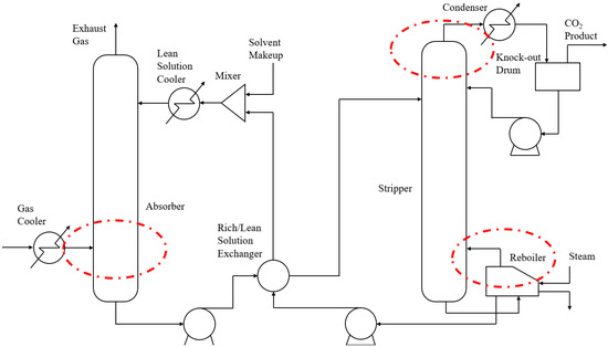
Figure 1.
Process scheme of a chemical absorption PCC system and its key positions.
3. Model Description
This section presents a hybrid model of an amine-based carbon capture system, the process scheme of which is shown in Figure 1. The absorber and the stripper within the system are the focus of modeling, and the properties of the solution are essential for the modeling process.
Firstly, how to use the results of key component inlets and outlets to calculate the solution properties within the framework of the three-parameter method is explained. Then, an equilibrium-based model is built based on the solution properties for both the absorber and the stripper. Additionally, the condensers, coolers, pumps, and heat exchangers are also essential components and are briefly modeled. All of these unit models have been integrated to form a comprehensive model.
3.1. Mass Transfer Model
The plug flow reactor (PFR) model is used to represent packed columns [20], assuming that the distributions of radial temperature, concentration, and velocity are consistent. For the mechanism model, the component mass balances for the vapor and liquid phases are, respectively, as follows:
where and are the vapor and liquid holdup, is the concentration of component , and are vapor and liquid velocities, is the flux of component between vapor and liquid phase, and is the vapor–liquid interfacial area, which is decided by the packing properties.
To calculate the component fluxes between different phases, the equilibrium pressure and the partial pressure are needed:
is the total mass transfer coefficient, is the equilibrium pressure in the liquid phase, and is the partial pressure of each component in vapor phase.
As the phase change of the solvent can be ignored in the process, the component fluxes are mainly about CO2 and H2O. The partial pressure in the vapor phase is as follows:
is the mole concentration of component in vapor phase. When using an ideal gas model, it equals the volume fraction. is the total pressure of the gas. The equilibrium pressure in the liquid phase is as follows:
is the saturated vapor pressure of water. It is a function only related to temperature. is the free H2O mole fraction in the liquid phase, and is the activity coefficient. They can be regarded as constant in the process.
To describe the equilibrium pressure of CO2, we can use the following:
is the Henry’s law constant. is the free CO2 mole fraction. is the activity coefficient. However, when facing complex or even unknown solutions, these parameters remain elusive. Therefore, the goal is to select a suitable model to characterize the properties of the solution and calculate the corresponding parameters using actual operating data for subsequent modeling processes. Vapor–liquid equilibrium is crucial for presenting solvent properties that influence the performance of a CO2 capture process. The general form of the vapor–liquid equilibrium formula assumes that the equilibrium CO2 partial pressure is a function of carbon loading and temperature, [21]. Carbon loading, α, is defined as the ratio of the total mole quantity of apparent CO2 to the total mole quantity of apparent absorbent solute in the solvent. A three-parameter formula was proposed by Oyenekan et al. [22,23]. It was first proposed as a six-parameter formula. In order to improve the accuracy of the calculations, a polynomial is used to describe the effect of temperature, leading to the development of the three-parameter form of this formula for generic solvent modeling. Plesu et al. [24] demonstrated that the three-parameter vapor–liquid equilibrium model is sufficient to accurately reproduce the behavior of a specific solvent. However, the application of this method is still limited to solutions with known properties. Jin et al. [25] provided mechanistic evidence that this model is universal and applicable to all solutions.
reflects the solvent properties. The term can serve as a criterion to denote absorption performance. Under the conditions of the same temperature, carbon loading, and absorption heat, a bigger means a bigger equilibrium CO2 partial pressure. Thus, an increasing stands for a decreasing absorption performance. The term characterizes the degree of carbon load transformation under a different temperature. All else being equal, a bigger means a smaller change in carbon load during the absorption–desorption process. It can be used as an index to measure the circulating capacity of the absorbent. represents the absorption heat of the reaction. It determines the temperature rise when the absorber absorbs CO2 and the amount of energy required to desorb the same mass of CO2 in the stripper. The gas–liquid equilibrium data with surrogate amine solutions have been returned to Equation (7), and the results have been compared with the experimental data. It is found that the feasibility of the three-parameter VLE model has been verified.
Therefore, the objective of this method is to obtain the CO2 partial pressure expression in the form of a three-parameter VLE model of the circulating solution through the actual operating data of the system. This CO2 partial pressure is then used to model the PCC system. In the process of solving the pressure expression, additional assumptions are necessary.
To calculate the component fluxes between different phases, the mass transfer coefficient is also required. This coefficient is influenced by the size parameters of packings and the properties of the solvents. However, when the mass transfer rate is sufficiently high, it primarily affects the temperature distribution and vapor–liquid phase composition within the column, without impacting the vapor–liquid phase equilibrium at the inlet and outlet. In most real systems, the mass transfer rate is adequate, and the design dimensions of the tower allows for sufficient mass transfer in the gas–liquid phase. Therefore, it will be assumed in the following analysis that vapor–liquid phase equilibrium is achieved at the inlet and outlet of the column.
3.2. Solvent Properties Calculation
As mentioned before, it can be assumed to reach vapor–liquid equilibrium at three positions, as shown in Figure 2: (1) solution outlet with a rich load in the absorber; (2) the gas outlet of the stripper; (3) the solution outlet with a lean load in the reboiler, which means the following:
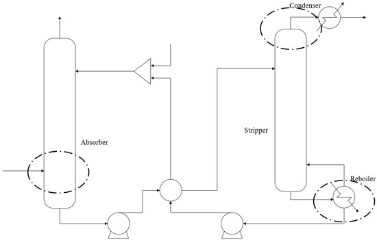
Figure 2.
Three positions with vapor–liquid equilibrium.
For the gas outlet of the stripper, when the system is under steady-state operating conditions, it only contains H2O and CO2, which are absorbed and desorbed throughout the entire process. The pressure in the different phase can be calculated from the following:
is the mass flow rate and represents the total capture amount of CO2. is the total pressure at the top of the stripper. As it reaches vapor–liquid equilibrium,
This result would be used in the whole process.
For the solution outlet with a lean load in the reboiler, the vapor phase composition only includes H2O and CO2. A three-parameter formula can be built to describe the equilibrium pressure of CO2:
For the solution outlet with a rich load in the absorber, there are CO2, H2O, and other insoluble gases, normally N2 and O2, in the vapor phase. As insoluble gas accounts for around 60–70% of the vapor volume, it can be assumed that the total mass flow rate of gas remains constant at the solution outlet of the absorber. The CO2 pressure can be calculated as follows:
From (13)–(16), parameter is eliminated:
Notice that is the load change of the system during the absorption and desorption process. It can be calculated by the total capture amount of CO2.
is the solute mass in the solution, which can be estimated from the system circulation flow rate and the solution mass fraction during initial solution configuration; is the relative molecular weight of the solute, which remains unchanged during system operation. The calculation of can be moved into To define a new load, we can use the following:
This equation contains two unknowns. Multiple sets of steady-state operating conditions can be obtained from the actual operating data of the system. After organizing and regressing the data of multiple sets of steady-state operating conditions, two unknowns can be calculated.
In the three-parameter formula for CO2 equilibrium pressure, the selection of only serves as an intercept, so a data point can be selected as the reference working condition. Since the pressure estimation of the reboiler is more accurate, the vapor liquid phase equilibrium at the outlet of the reboiler shall prevail, and it may be assumed that the lean liquid load is a certain number, . The parameter can be calculated through the selection of the reference working condition. In the previous mechanism model, the absolute value of the solution load needs to be accurately calculated, because this will affect the calculation of the rate of CO2 absorption. However, in this method, it is assumed that the gas–liquid phase equilibrium is always satisfied, so there is no need to calculate the absorption rate. At this time, the absolute value of the solution load is no longer important. What is really important is the difference between the rich and lean solvent load during the cycle, which determines the total absorption amount. It is feasible to use this reference load to calculate the parameter .
Based on this, three parameters of the vapor–liquid equilibrium formula are obtained, which can preliminarily estimate the physical properties of the solution.
It should be noted that the three-parameter formula has also been developed in the process. The definition of load changed from the ratio of molar quantity to the ratio of molar quantity to mass. Since the relative molecular mass of CO2 is determined, this is also actually the ratio of the mass of CO2 to the amine. With this new definition, the parameter includes the effect of the relative molecular mass of the solvent. This solves problems that may arise when faced with unknown solvents.
3.3. Energy Balance
After obtaining the parameters related to the equilibrium pressure of the solution, it is also essential to calculate the heat capacity of the solution by establishing an energy balance. The material and energy flows of the absorber and stripper are illustrated in Figure 3.
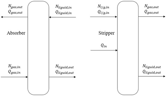
Figure 3.
Energy balance for absorber and stripper.
For the absorber, there is no energy input, and the heating comes entirely from the heat generated by CO2 absorption. At the same time, there is also an energy change in the phase transition of H2O. Taking the entire tower as a whole, the energy balance relationship is obtained.
is the heat capacity of the solution and is influenced by the solute type and concentration. is the heat capacity of the gas mixture. In terms of composition, the temperature and pressure of the gas can be determined, so the heat capacity can be calculated. is the latent heat of water and can be seen as constant (48,000 kJ/kmol) in the process.
For the stripper, its energy input is the heat duty of the reboiler, which is converted into the reaction heat of CO2 desorption, the latent heat of vaporization of H2O, and the sensible heat of the solution temperature increase. In terms of the feed to the stripper, the rich liquid at the outlet of the absorption tower will receive heat from the high-temperature lean liquid at the outlet of the reboiler after passing through the heat exchanger. Pre-desorption will occur after heating, resulting in a rich liquid flow containing both liquid and vapor phases entering the stripper. The estimation of the pre-desorption situation has a significant impact on the overall energy balance calculation of the stripper. The vapor–liquid equilibrium formula obtained from the aforementioned process is used to estimate the pre-desorption gas volume at the inlet of the stripper.
At the inlet of the stripper, the following is true:
The pre-desorption amount of CO2 can be calculated from . And the relationship between the mass flow rates of H2O and CO2 at the inlet is as follows:
The energy balance relationship is obtained:
According to the above, the energy balance equations for the absorber and stripper are formulated separately. is considered to be a constant value. And is calculated by the mass balance of the inlet and the outlet of the column. Therefore, it is a set containing two unknowns, . It can be solved using data from only one operating point, but in order to improve the accuracy of the calculation and maximize the utilization of operating data, a regression calculation method using multiple sets of operating conditions is used to solve.
3.4. Iterative Calculation
The important parameter of reaction heat is obtained in the calculation of vapor–liquid phase equilibrium and energy balance. It is noted that the CO2 partial pressure formula obtained from the equilibrium is used in the energy balance to calculate the pre-desorption at the inlet of the stripper. The relationship of the inlet of the stripper and outlet of the stripper can be described as follows:
From (29) and (30), parameter is eliminated; then, we can use (21) to replace :
This expression is similar to the equation . When if the estimation of reaction heat () in the equilibrium formula is too small, it will result in the calculated being too big and a higher reaction heat being obtained in the calculation of energy balance. The theoretical proof of this equation has not been completed, but it can be inferred from the actual data substitution that this relationship is satisfied. After the energy balance calculation, it is necessary to iterate the calculated reaction heat term into the formula, adjust the three-parameter model after regression, and improve the estimation accuracy of the model.
3.5. Equilibrium-Based Model Building
After characterizing the properties of the solution using data, the entire system can be constructed. As the physical properties required for modeling are obtained from the assumption of equilibrium, the model is an equilibrium-based model.
The plug flow reactor (PFR) is used, which assumes that the distribution of radial temperature, concentration, and velocity are consistent. The pressure drop in the packed column is ignored, meaning the entire tower operates at the same pressure. Since the pressure is relatively low in the absorber and stripper, the gas is treated as being in an ideal phase.
Mass and heat transfer are described by the two-film theory. The fluxes of CO2 and H2O between the two phases are considered in both directions. It is assumed that the mass transfer rate is infinitely large, allowing the gas–liquid phase in each stage to reach equilibrium. The mass transfer is determined by the amount that can achieve this equilibrium.
3.6. Modelling of Other Components
In addition to the tower components, the entire system also requires auxiliary components such as condensers, heat exchangers, and pumps. During the modeling process, these components were simplified. The condenser is designed to maintain the outlet solution at a specific temperature, while the pump ensures that the outlet solution is maintained at a designated pressure. The temperature difference between the cold and hot ends of the heat exchanger is a predetermined value, calculated from actual temperature data. Energy conservation is upheld throughout the heat exchange process. For the pre-desorption scenario at the outlet of the hot rich liquid, calculations are based on the previously determined CO2 equilibrium pressure and the saturated vapor pressure of water. Various components are interconnected to create a comprehensive carbon capture system model. The input parameters for this model include flue gas characteristics, absorption liquid properties, pressures in the absorber and stripper, and the heat load at the reboiler.
3.7. Applications of the Model
The most critical assumption made in the model is that it achieves vapor–liquid phase equilibrium at both the inlet and outlet of the column. Therefore, the model necessitates that the absorbent exhibits a sufficient reaction rate, or that the system is equipped with a device of adequate size, which is typically achieved in practical applications. While the traditional process system is employed to elucidate the method in this study, the balance of component positions consistently exists across systems with varying processes, thereby expanding the model’s applicability. However, it also necessitates accurate data regarding the locations of these essential components.
It should be noted that in the process of calculation and regression, the reciprocal difference between the outlet temperature of the absorber and the temperature of the reboiler is implemented. The temperature increase of the solution after the absorption of CO2 in the absorber is limited and is influenced by the gas–liquid ratio and the heat of the absorption reaction. The temperature of the reboiler is affected by the pressure of the stripper. This indicates that the method should be applied with data points at different stripper pressures, or with the results of different absorption states of the system, to make the reboiler temperature vary greatly at different data points.
4. Model Validation
For unknown solvents, even if the characteristic parameters are obtained by this method, the accuracy of the method still cannot be verified. A traditional chemical absorption process was established in Aspen PLUS V11 to verify this method. The solution used in the system is DEA, which was fully studied in previous studies. The characteristic parameters of the solution were extracted from the model data and compared with the actual values. At the same time, the availability and accuracy of the data were ensured. The model is shown in Figure 4. The system consists of components including an absorption tower, heat exchanger, stripper, pump, etc. Although specific size parameters will not be used in the application of this method, as it is an equilibrium-based model, they are still presented in Table 1.
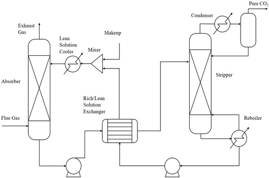
Figure 4.
Traditional chemical absorption process model in Aspen.

Table 1.
Device parameters and packing material.
We let the system run in the cases shown in Table 2. The four cases were under the same absorber pressure and stripper pressure. For the lean solvent flow rate, the low value was 30,000 kg/h and the high value was 50,000 kg/h. For the inlet flue gas flow rate, the low value was 6300 kg/h and the high value was 8000 kg/h. The input reboiler power was therefore different. With these import parameters, the outlet results were also obtained and are shown in the table below.
Table 2.
Import parameters and results in different cases.
After undergoing the calculation using the above method, the three-parameter formula and the heat capacity for the solution was obtained. The iteration relationship was also verified:
To obtain the properties of a 30% DEA solution using the three-parameter formula framework, the actual CO2 equilibrium pressure under different conditions was obtained through Aspen. The temperature, load, and equilibrium pressure values were then regressed to determine the three parameters, as shown in Figure 5. These parameters were considered as the actual values of the properties of the 30% DEA solution.
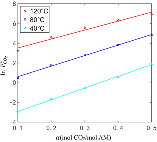
Figure 5.
Equilibrium pressure for DEA.
The calculated result is compared with the actual value obtained through regression analysis in Table 3. The accuracy of , , and demonstrates the effectiveness of this method. As previously mentioned, a deviation exists between the calculated and actual values of parameter due to the selection of the solution load under basic operating conditions. This example demonstrates the effectiveness and accuracy of the method in determining the properties of unknown solutions while maintaining a clear and logical structure.
Table 3.
Comparison of calculated and actual values.
Figure 6 shows the change in reboiler temperature of the 30 wt% DEA solution under different stripper pressure. The difference between the upper and lower limits is about 20 °C. This may lead to the difference in the reciprocal being too small, affecting the accuracy of the calculation.
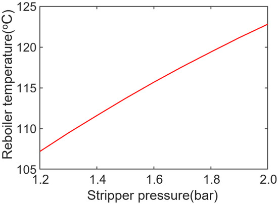
Figure 6.
The 30 wt% DEA boiling temperature varies with stripper pressure.
Then, we used the properties obtained to build the CO2 capture system. To demonstrate the accuracy of the model, the inlet conditions were selected to match the gas and liquid flow rates, as shown in Table 4. For the operating pressure of the stripper, 1.4 bar was chosen, which is lower than the dataset pressure. For the heat load of the reboiler, 500 kW was chosen, which means inadequate desorption. In addition to the overall capture rate of the system, which is of most concern, the temperature of the hot rich liquid at the outlet of the reboiler and the temperature of the flue gas at the top outlet of the stripper were also verified. The verification results are shown in Figure 7. The average relative error of the capture rate was 5.6%. This method can accurately calculate the temperature at the inlet and outlet of each component and the total CO2 capture rate of the system when the inlet flow rate and reboiler heat load are known.
Table 4.
Input parameters of verification point.
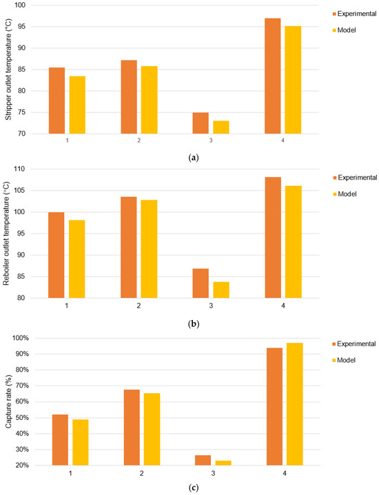
Figure 7.
Comparison of model results: (a) the temperature of the hot rich liquid at the outlet of the reboiler; (b) the temperature of the flue gas at the top outlet of the stripper; (c) the total carbon capture rate.
5. Case Study
The actual system usually uses a more complex solution to improve the system’s capture rate and reduce the system’s operating cost. If using existing methods, it is impossible to model the system. The proposed method can be applied to this scenario. Here, this method was used in the modeling process of a pilot plant in Jiangsu Province. The capacity of this system is 10,000 tons of CO2 per year. It uses the traditional process and uses a new type of solvent. As this solution was developed by a research unit and has patent protection, for the plant, this solvent remains unknown. However, there is still a need for power plants to establish models for carbon capture systems.
Figure 8 shows the absorption liquid flow rate and the CO2 flow rate curve of the power plant during a shutdown phase on a certain day. A steady-state data point is selected when the operating data are stable near a certain value. After acquiring multiple steady-state data points, this method can be applied to analyze the actual system. The operational data selected are presented in Table 5.
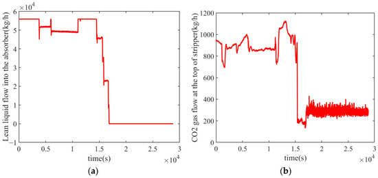
Figure 8.
Operation data of the system shutdown phase on a certain day: (a) lean liquid flow into the absorber; (b) CO2 gas flow at the top of the stripper.
Table 5.
Operational data of the pilot plant.
As the solvent still remains unknown to us, it was impossible to compare the model result with the result calculated using the equilibrium data of the solvent. It was compared with the traditional solvent, and we evaluated the properties of the solution. In this method, the results of parameter are related to the selection of the benchmark load, which was not compared.
As shown in Figure 9, this new type of absorbent has lower absorption heat and lower cycle capacity compared to traditional ones. This result demonstrates the advantages and disadvantages of this new solution. And this indicates that for a new type of solution, lower absorption heat (smaller ) and higher cyclic carbon capacity (smaller ) are better characteristics.
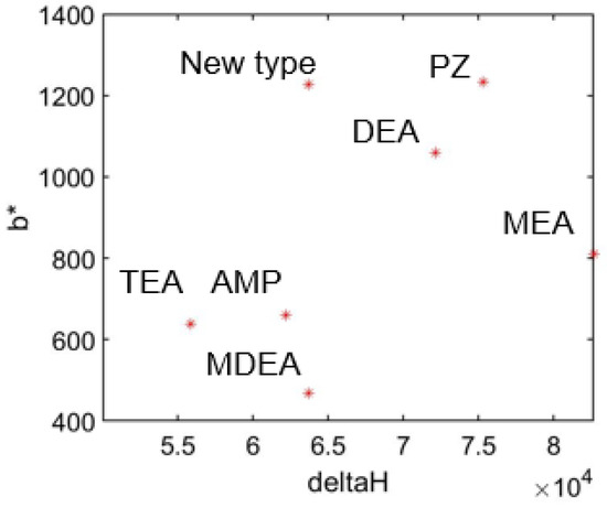
Figure 9.
Comparison of solution properties.
Next, the overall model accuracy was verified in Figure 10, still considering the system’s carbon capture rate. The average relative error of the built model’s capture rate was 3.0%, and the accuracy was able meet the simulation requirements. This method can be used for actual system modeling and simulation of unknown solutions.
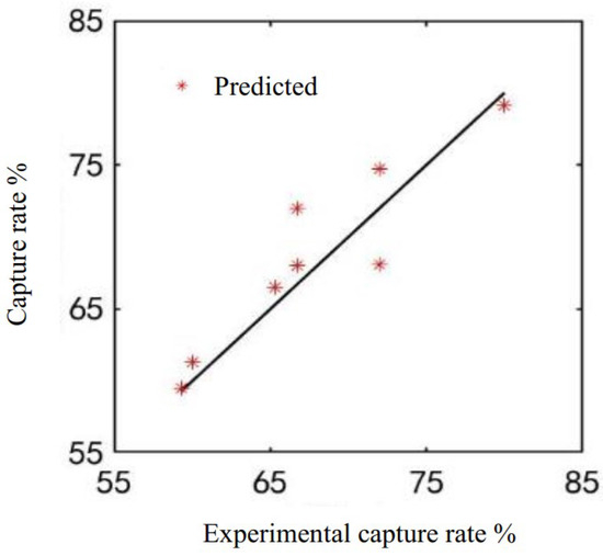
Figure 10.
Model accuracy verification.
6. Conclusions
This paper proposes a hybrid modeling method that combines data and a mechanism. Within the framework of the three-parameter method, the unknown solution properties can be characterized using operating data. On this basis, modeling based on an equilibrium can solve the modeling problem of an actual carbon capture system. The comparison results between modeling and the simulator built in Aspen, which serves as an actual system, show that the estimated solvent properties are in good agreement with the actual value. Meanwhile, the results indicate that the model has good accuracy and can be used for simulation research. The case study of modeling for the carbon capture system in Jiangsu Province shows that this method can also be used to evaluate the properties of new solutions. The new type of absorbent has lower absorption heat and lower cycle capacity compared to traditional ones. It should be noted that this method is applicable to the condition that the mass transfer rate is sufficient. In order to improve the accuracy of the calculation, it is necessary to select data points with large changes in the temperature of the reboiler.
In future research, the dynamic characteristics of the system will be the focus of research. How to calculate the CO2 reaction rate of the solution and the temperature and flow during the flow process, using dynamic data from the actual system, may represent a promising direction for future studies. Since this method assumes gas–liquid phase equilibrium, mass transfer rates can be considered to establish dynamic models in the future. This also puts forward higher requirements for data quality.
Author Contributions
Conceptualization, Z.L.; Methodology, S.J.; Software, S.J.; Writing—original draft, S.J.; Writing—review & editing, P.L.; Supervision, Z.L. All authors have read and agreed to the published version of the manuscript.
Funding
This research was funded by the National Key Research and Development Program of China (2023YFC3807201) and the Phase IV Collaboration between BP and Tsinghua University.
Data Availability Statement
The original contributions presented in this study are included in the article. Further inquiries can be directed to the corresponding author.
Conflicts of Interest
The authors declare no conflict of interest.
References
- United Nations. Paris Agreement. 2015. Available online: https://www.un.org/en/node/84376 (accessed on 4 July 2024).
- Wu, C.; Huang, Q.; Xu, Z.; Sipra, A.T.; Gao, N.; Vandenberghe, L.P.d.S.; Vieira, S.; Soccol, C.R.; Zhao, R.; Deng, S.; et al. A Comprehensive Review of Carbon Capture Science and Technologies. Carbon Capture Sci. Technol. 2024, 11, 100178. [Google Scholar] [CrossRef]
- Xu, Y.; Luo, C.; Sang, H.; Lu, B.; Wu, F.; Li, X.; Zhang, L. Structure and Surface Insight into a Temperature-Sensitive CaO-Based CO2 Sorbent. Chem. Eng. J. 2022, 435, 134960. [Google Scholar] [CrossRef]
- Dunstan, M.T.; Donat, F.; Bork, A.H.; Grey, C.P.; Müller, C.R. CO2 Capture at Medium to High Temperature Using Solid Oxide-Based Sorbents: Fundamental Aspects, Mechanistic Insights, and Recent Advances. Chem. Rev. 2021, 121, 12681–12745. [Google Scholar] [CrossRef] [PubMed]
- Sofia, D.; Giuliano, A.; Poletto, M.; Barletta, D. Techno-Economic Analysis of Power and Hydrogen Co-Production by an IGCC Plant with CO2 Capture Based on Membrane Technology. In Computer Aided Chemical Engineering; Elsevier: Amsterdam, The Netherlands, 2015; Volume 37, pp. 1373–1378. [Google Scholar] [CrossRef]
- Xu, Y.; Donat, F.; Luo, C.; Chen, J.; Kierzkowska, A.; Awais Naeem, M.; Zhang, L.; Müller, C.R. Investigation of K2CO3-Modified CaO Sorbents for CO2 Capture Using in-Situ X-ray Diffraction. Chem. Eng. J. 2023, 453, 139913. [Google Scholar] [CrossRef]
- Wu, X.; Wang, M.; Liao, P.; Shen, J.; Li, Y. Solvent-Based Post-Combustion CO2 Capture for Power Plants: A Critical Review and Perspective on Dynamic Modelling, System Identification, Process Control and Flexible Operation. Appl. Energy 2020, 257, 113941. [Google Scholar] [CrossRef]
- Aghel, B.; Janati, S.; Wongwises, S.; Shadloo, M.S. Review on CO2 Capture by Blended Amine Solutions. Int. J. Greenh. Gas Control. 2022, 119, 103715. [Google Scholar] [CrossRef]
- Janati, S.; Aghel, B.; Shadloo, M.S. The Effect of Alkanolamine Mixtures on CO2 Absorption Efficiency in T-Shaped Microchannel. Environ. Technol. Innov. 2021, 24, 102006. [Google Scholar] [CrossRef]
- Endo, T.; Kajiya, Y.; Nagayasu, H.; Iijima, M.; Ohishi, T.; Tanaka, H.; Mitchell, R. Current Status of MHI CO2 Capture Plant Technology, Large Scale Demonstration Project and Road Map to Commercialization for Coal Fired Flue Gas Application. Energy Procedia 2011, 4, 1513–1519. [Google Scholar] [CrossRef]
- Singh, A.; Stéphenne, K. Shell Cansolv CO2 Capture Technology: Achievement from First Commercial Plant. Energy Procedia 2014, 63, 1678–1685. [Google Scholar] [CrossRef]
- Jin, H.; Liu, P.; Li, Z. Energy-Efficient Process Intensification for Post-Combustion CO2 Capture: A Modeling Approach. Energy 2018, 158, 471–483. [Google Scholar] [CrossRef]
- Baburao, B.; Craig, S. Advanced Intercooling and Recycling in CO2 Absorption. U.S. Patent 8,460,436 B2, 11 June 2013. [Google Scholar]
- Kvamsdal, H.M.; Jakobsen, J.P.; Hoff, K.A. Dynamic Modeling and Simulation of a CO2 Absorber Column for Post-Combustion CO2 Capture. Chem. Eng. Process. Process Intensif. 2009, 48, 135–144. [Google Scholar] [CrossRef]
- Zhu, M.; Wu, X.; Shen, J.; Lee, K. Dynamic Modeling, Validation and Analysis of Direct Air-Cooling Condenser with Integration to the Coal-Fired Power Plant for Flexible Operation. Energy Convers. Manag. 2021, 245, 114601. [Google Scholar] [CrossRef]
- Lawal, A.; Wang, M.; Stephenson, P.; Koumpouras, G.; Yeung, H. Dynamic Modelling and Analysis of Post-Combustion CO2 Chemical Absorption Process for Coal-Fired Power Plants. Fuel 2010, 89, 2791–2801. [Google Scholar] [CrossRef]
- Li, F.; Zhang, J.; Oko, E.; Wang, M. Modelling of a Post-Combustion CO2 Capture Process Using Neural Networks. Fuel 2015, 151, 156–163. [Google Scholar] [CrossRef]
- Abdul Manaf, N.; Cousins, A.; Feron, P.; Abbas, A. Dynamic Modelling, Identification and Preliminary Control Analysis of an Amine-Based Post-Combustion CO2 Capture Pilot Plant. J. Clean. Prod. 2016, 113, 635–653. [Google Scholar] [CrossRef]
- Akinola, T.E.; Oko, E.; Gu, Y.; Wei, H.-L.; Wang, M. Non-Linear System Identification of Solvent-Based Post-Combustion CO2 Capture Process. Fuel 2019, 239, 1213–1223. [Google Scholar] [CrossRef]
- Gaspar, J.; Jørgensen, J.B.; Fosbøl, P.L. A Dynamic Mathematical Model for Packed Columns in Carbon Capture Plants. In Proceedings of the 2015 European Control Conference (ECC), Linz, Austria, 15–17 July 2015; pp. 2738–2743. [Google Scholar] [CrossRef]
- Chen, X.; Closmann, F.; Rochelle, G.T. Accurate Screening of Amines by the Wetted Wall Column. Energy Procedia 2011, 4, 101–108. [Google Scholar] [CrossRef]
- Oyenekan, B.A.; Rochelle, G.T. Energy Performance of Stripper Configurations for CO2 Capture by Aqueous Amines. Ind. Eng. Chem. Res. 2006, 45, 2457–2464. [Google Scholar] [CrossRef]
- Oyenekan, B.A.; Rochelle, G.T. Alternative Stripper Configurations for CO2 Capture by Aqueous Amines. AIChE J. 2007, 53, 3144–3154. [Google Scholar] [CrossRef]
- Plesu, V.; Bonet i Ruiz, J.; Bonet Ruiz, A.; Chavarria, A.; Iancu, P.; Llorens Llacuna, J. Surrogate Model for Carbon Dioxide Equilibrium Absorption Using Aqueous Monoethanolamine. Chem. Eng. Trans. 2018, 70, 919–924. [Google Scholar] [CrossRef]
- Jin, H.; Liu, P.; Li, Z. Impact of Solvent Properties on Post-Combustion Carbon Capture Processes: A Vapor–Liquid Equilibrium Modelling Approach. Chem. Eng. Sci. X 2021, 10, 100095. [Google Scholar] [CrossRef]
Disclaimer/Publisher’s Note: The statements, opinions and data contained in all publications are solely those of the individual author(s) and contributor(s) and not of MDPI and/or the editor(s). MDPI and/or the editor(s) disclaim responsibility for any injury to people or property resulting from any ideas, methods, instructions or products referred to in the content. |
© 2025 by the authors. Licensee MDPI, Basel, Switzerland. This article is an open access article distributed under the terms and conditions of the Creative Commons Attribution (CC BY) license (https://creativecommons.org/licenses/by/4.0/).