Tool Wear State Monitoring in Titanium Alloy Milling Based on Wavelet Packet and TTAO-CNN-BiLSTM-AM

Abstract

To effectively monitor the nonlinear wear variation of tools during the processing of titanium alloys, this study proposes a hybrid deep neural network fault diagnosis model that integrates the triangulation topology aggregation optimizer (TTAO), convolutional neural network (CNN), bidirectional long short-term memory network (BiLSTM), and attention mechanism (AM). Firstly, vibration signals from the machine tool spindle are acquired and subjected to the wavelet packet transform (WPT) to extract multi-frequency band energy features as model inputs. Then, the CNN and BiLSTM modules capture the features and temporal relationships of the input signals. Finally, introduction of the AM, combined with the TTAO algorithm, automatically extracts deep features, overcoming issues such as local optima and slow convergence in traditional neural networks, thereby enhancing the accuracy and efficiency of tool wear state recognition. The experimental results demonstrate that the proposed model achieves an average accuracy rate of 98.649% in predicting tool wear states, outperforming traditional backpropagation (BP) networks and standard CNN models.

1. Introduction

Titanium alloys are widely used in aerospace, military equipment, medical devices, and other industries due to their high specific strength and stiffness, excellent high-temperature strength and low-temperature performance, good corrosion resistance, and strong heat resistance [1,2,3]. However, the poor thermal conductivity of titanium alloys makes cutting heat difficult to dissipate, resulting in extremely high cutting temperatures during milling. Moreover, their high chemical reactivity leads to biochemical reactions with cutting tools at high temperatures, causing severe work hardening phenomena. This leads to rapid tool wear and reduced tool life, with tool maintenance costs accounting for 15% of total production costs [4]. Therefore, accurately identifying tool wear states, selecting the optimal time for tool replacement, and regrinding tools are of significant practical importance for reducing titanium alloy processing costs and achieving efficient, low-carbon processing.

Tool wear monitoring methods in milling can be categorized into direct and indirect methods. Direct methods measure the surface morphology of milling tools using mediums such as light and ultrasonic waves, providing reliable results but involving cumbersome processes. For instance, Guo et al. [5] proposed a 3D imaging technique based on stroboscopic stereophotography, enabling direct geometric measurements of cutting tools through industrial cameras. Fong et al. [6] utilized industrial cameras to capture tool wear images and constructed a novel quantitative image tool wear measurement system based on cross-correlation analysis. Bergs et al. [7] researched tool wear image processing methods based on deep learning, using CNNs to classify tool types and accurately categorize wear states of ball-end mills, end mills, and drills. However, direct methods can only perform offline monitoring after machine shutdown, making real-time dynamic monitoring of tool wear challenging, which adversely affects production efficiency in actual processing.

Indirect methods involve collecting signals such as force, heat, vibration, sound, and power generated during the titanium alloy milling process, analyzing and processing these signals to extract feature information related to tool wear states, and establishing their corresponding relationships with tool wear states. These methods have lower monitoring costs and less impact on processing efficiency. Currently, the combination of indirect measurement of collected signal features with neural networks for online identification of milling tool wear has gained extensive research attention [8].

To effectively extract milling tool wear features from collected signals, researchers have proposed numerous tool wear recognition techniques in recent years. Rimpault et al. [9] analyzed cutting force signals of carbon fiber-reinforced plastics (CFRPs) and proposed an adaptive method based on fractal analysis to estimate tool wear and evaluate workpiece surface quality. Kunal et al. [10] collected milling force signals and milling surface textures, and by combining histogram variance of milling surface texture parameters with synthetic cutting force data using the Kalman filter method to establish a model predicting flank wear, they achieved good accuracy. Klocke et al. [11] proposed a tool wear state recognition method based on acoustic emission signals, using k-means clustering to classify tool wear conditions within selected frequency ranges. Through step drilling experiments, the model could detect the spectral features and wear conditions of each engaged cutting edge. Niaki et al. [12] extracted spindle power signals and used Kalman filters to track tool flank wear area transformations during cutting under variable conditions, modeling tool wear area evolution using third-order polynomial empirical functions to study tool wear laws under higher wear conditions. However, signals like force, sound, and power are susceptible to noise interference during acquisition and are challenging to collect, leading to lower recognition accuracy. Therefore, more researchers are choosing vibration signals during tool milling as the primary signal source for monitoring tool wear states.

Cao et al. [13] collected spindle vibration signals as tool wear signals, stacked reconstructed signal sequences of different scales and their Hilbert envelope demodulation spectra, constructed 2D signal matrices for training and testing CNN models, and achieved tool wear state recognition in end milling experiments with different processing parameters. Upase et al. [14] collected vibration signals during hard steel turning and achieved accurate prediction of tool wear using an artificial neural network model. Zhou et al. [15] studied three-directional cutting vibration signals of spindles, evaluated their dynamic performance through pulse tests and modal analysis, quantified slight waveform deformations of signals using ambiguity analysis, associated them with different tool wear conditions, and established a tool condition monitoring system based on support vector machine (SVM), demonstrating that the obtained features could serve as tool wear characteristics. However, these research methods mostly use small sample data, making it difficult to apply to modal recognition problems requiring large sample inputs for deep learning models.

Many researchers have studied data-driven tool wear prediction models based on deep learning (DL), which can process complex sensor signals and have high feature representation capabilities [16,17]. Among them, recurrent neural networks (RNNs), CNNs, and their variants are widely used for online prediction of tool wear, capable of taking multivariate time series data as input. Gouarir et al. [18] converted force signals into two-dimensional images based on Gramian angular fields (GAF), smoothed and dimensionally reduced the images using piecewise aggregate approximation, and used CNNs to predict tool wear states. To ensure the accuracy of tool wear prediction and improve manufacturing sustainability, Wang et al. [19] proposed a probability method based on particle filtering, effectively combining uncertainty and online measurements to predict tool wear states. Wang et al. [20] proposed a deep heterogeneous GRU model combining local feature extraction for predictive analytics of tool wear in intelligent manufacturing. Sun et al. [21] proposed a deep learning-based method for predicting tool wear states during processing using LSTM networks and residual CNNs (ResNet) for real-time tool wear prediction to support data-driven tool replacement decisions in intelligent manufacturing. Shi et al. [22] proposed a tool wear prediction method based on deep learning using multiple stacked sparse autoencoders to capture vibration signals for deep feature learning and multi-feature fusion. Sick et al. [23] and Zhu et al. [24] emphasized the superiority of artificial neural networks and the Wavelet Transform in tool condition monitoring (TCM).

Recent studies have made notable progress in the field of tool wear monitoring by introducing advanced methods and frameworks. For instance, Liu et al. [25] proposed domain-adversarial neural networks with multiple loss collaborative optimization to address the challenges of adapting models to different machining conditions. This method utilizes ResNet18 for feature extraction and optimizes model loss convergence to achieve high recognition accuracy with reduced training time. Another approach by Mishra et al. [26] employed Gaussian mixture models based on signal indicators derived from the physics of machining, such as energy and magnitude, to classify tool wear states. This method achieved high classification accuracy (96.5%) and was validated across multiple datasets. Additionally, Liu et al. [27] conducted systematic reviews that highlighted the limitations of feature extraction and decision-making methods in industrial environments, emphasizing the need for robust anti-interference capabilities and improved real-time performance in tool wear monitoring. Advanced hybrid models, such as SBiLSTM with multi-head self-attention, demonstrated by Hao et al. [28], have shown the ability to adapt to different cutting conditions and improve accuracy by 23.84% compared to conventional methods. In predictive maintenance, Qiang et al. [29] proposed multi-source transfer learning frameworks that transfer knowledge between domains, enabling high prediction accuracy (over 93%) for tool life under varying operating conditions. Lastly, studies by Low et al. [30] on real-time tool wear monitoring in micro-milling emphasized the importance of integrating deep learning with high-fidelity digital twins to enhance real-time predictive capabilities.

However, the above methods still have some shortcomings in practical applications, such as low prediction accuracy, especially in complex working conditions where stable accuracy is hard to ensure. Additionally, these methods perform poorly in real time, making it difficult to adapt to dynamic changes during the cutting process and unable to achieve real-time dynamic monitoring of tool wear states. These limitations hinder their application in high-precision, high-efficiency manufacturing environments that demand real-time feedback and rapid adjustment.

To address these challenges, this study proposes a novel hybrid approach that combines the wavelet packet transform, convolutional and bidirectional long short-term memory networks, and the triangulation topology aggregation optimizer with an attention mechanism. Unlike previous studies, which often rely on domain-specific data or small datasets, our method integrates multi-scale feature extraction with advanced deep learning models to significantly enhance tool wear recognition. The wavelet packet transform provides comprehensive signal decomposition, capturing both high- and low-frequency components critical for analyzing non-stationary signals. The convolutional and bidirectional long short-term memory networks jointly learn spatial dependencies and bidirectional temporal relationships, effectively modeling the progressive nature of tool wear. Furthermore, the attention mechanism focuses on critical features in the signal, while the triangulation topology aggregation optimizer ensures efficient parameter tuning, avoiding issues such as slow convergence and local optima. The experimental results demonstrate that the proposed method achieved an average accuracy of 98.649%, surpassing existing techniques in both recognition accuracy and real-time adaptability. This innovation provides a reliable solution for intelligent manufacturing systems, meeting the demands of real-time monitoring, adaptive control, and robust performance under complex machining conditions.

Based on the above background, this paper proposes a hybrid model integrating the WPT and TTAO-CNN-BiLSTM-AM [31], aiming to improve the accuracy and real-time performance of tool wear state recognition by combining advanced optimization algorithms with deep learning models. The main contributions are as follows:

In this study, WPT is employed to perform multi-scale decomposition of vibration signals during the tool wear process, effectively extracting energy features across different frequency bands. Unlike the traditional wavelet transform, the WPT decomposes not only the low-frequency components of the signal but also the high-frequency components, enabling a more comprehensive capture of frequency characteristics. This is particularly suitable for analyzing complex and non-stationary vibration signals in titanium alloy milling. By applying a three-level WPT decomposition, the model effectively captures the frequency spectrum features at various stages of tool wear, laying a solid foundation for subsequent classification and recognition.

The proposed TTAO-CNN-BiLSTM-AM hybrid model utilizes CNN to extract spatial features from vibration signals, while BiLSTM captures temporal dependencies, and the AM further highlights key features to enhance recognition accuracy. The TTAO algorithm, by simulating a triangulation topology structure, improves the model’s global search capability, avoiding the local optima problem often encountered in traditional neural networks, and accelerates convergence. The experimental results show that this model achieved a tool wear state recognition accuracy of 98.649%.

The structure of this paper is as follows: Section 2 introduces the proposed methods, including the WPT, TTAO algorithm, and data acquisition experiments. Section 3 presents experimental validations for tool life prediction, demonstrating the effectiveness of the WPT and TTAO-CNN-BiLSTM-AM methods. Section 4 summarizes the paper.

2. Materials and Methods

The proposed tool wear state identification method based on the wavelet packet and TTAO-CNN-BiLSTM-AM includes data acquisition and preprocessing, feature extraction using the WPT, and model training and classification prediction. The diagnostic process is shown in Figure 1.

(1)

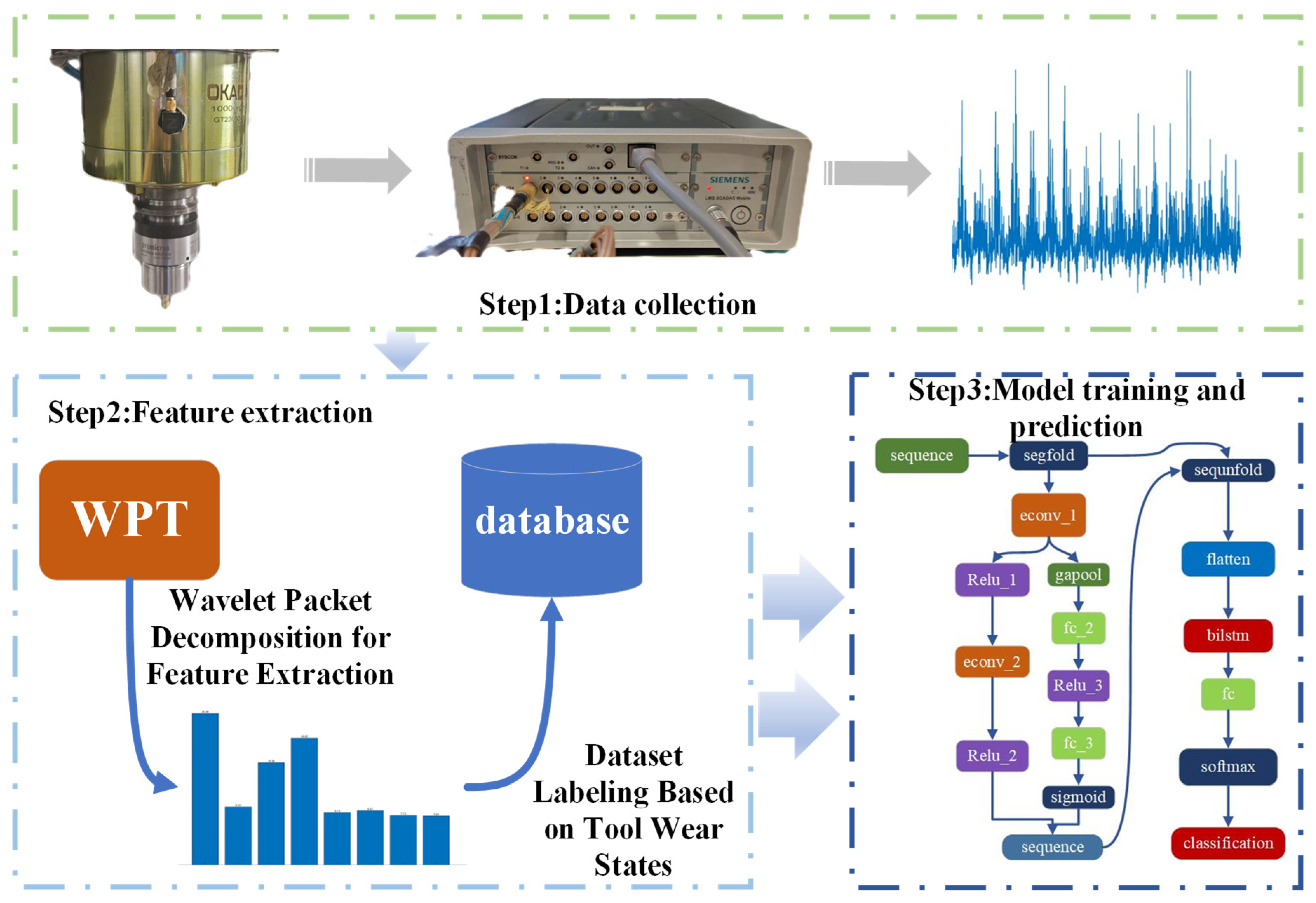
Data acquisition and preprocessing: Collect vibration signals during the tool cutting process using signal acquisition devices and perform noise reduction and segmentation to ensure data quality.

(2)

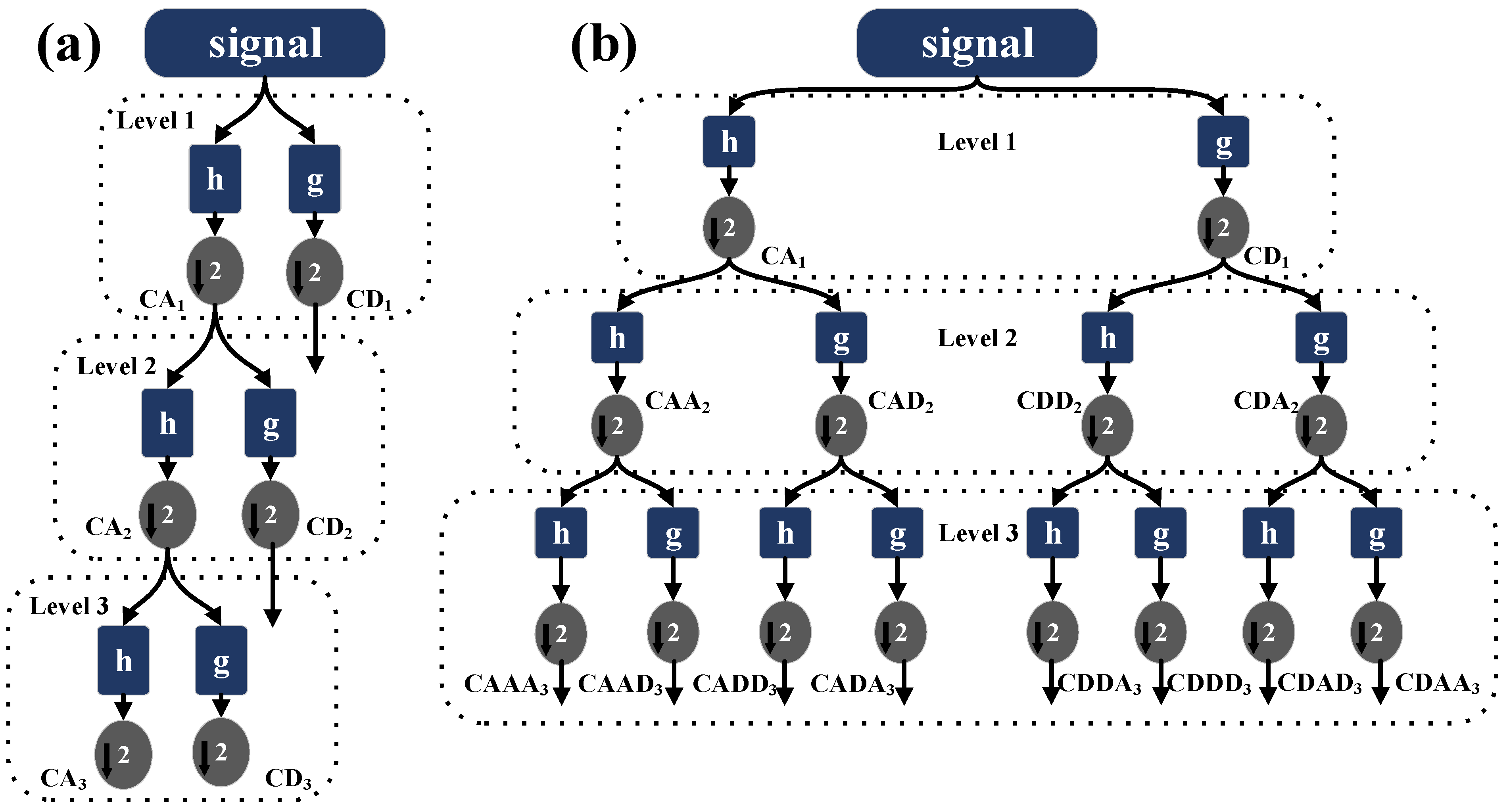
Feature extraction using WPT: Perform a three-layer WPT on the processed signals to extract energy distribution features.

(3)

Model training and classification prediction: Based on the eight extracted features from each signal group, divide the dataset into training and testing sets. Use the TTAO-CNN-BiLSTM-AM model to perform classification prediction and achieve fault type recognition.

2.1. Data Acquisition

In the tool milling process, the flank wear land width (VB) is closely related to processing quality and is commonly used as a judgment basis. According to ISO-8688-1/1994 [32], the tool wear limit is defined as uniform flank wear reaching 0.3 mm or non-uniform flank wear reaching 0.6 mm. Based on the changes in milling time and tool flank wear, the wear degree is divided into initial, normal, and rapid wear stages. At each wear stage during the entire milling process, a 10 s vibration signal is uniformly selected as the initial sample.

This study uses a V-850 CNC machine tool manufactured by Shenyang His Co., Ltd. (Shenyang, China) as the cutting experiment equipment. A tool milling vibration acquisition platform is constructed using the LMS Test. The Xpress Vibration and Noise Testing Analysis System from Siemens (Tokyo, Japan) is the main detection equipment, as shown in Figure 2.

The workpiece material is TC4 titanium alloy measuring 100 × 100 × 25 mm. The milling tool is an uncoated tungsten steel four-flute end mill with a diameter of 6 mm. The cutting parameters are as follows: cutting speed is 2000 r/min, feed rate is 200 mm/min, cutting depth is 0.5 mm, and cutting width is 1 mm. To accelerate tool wear, cutting is performed without cutting fluid. A three-axis acceleration sensor is installed on the outer wall of the CNC machine spindle to collect the machine’s vibration signals at a sampling frequency of 12.8 kHz and a sampling time of 10 s. The collected signals undergo the following preprocessing steps: signal formatting, segmentation, and noise filtering.

In this study, vibration spectrum analyzers are used to capture the vibration signals during tool milling. A total of 16,640 vibration data points are collected, with 11,648 randomly selected as training samples and 4992 selected as testing samples, maintaining a training-to-testing ratio of 7:3. The processed data are imported into the neural network model for tool wear state identification. Details are shown in

Table 1. Dataset distribution for training and test sets.

Dataset	Training Set	Test Set
1	3780	1620
2	2996	1284
3	4872	2088
Total	11,648	4992

.

2.2. Data Processing

Firstly, the raw signals collected by the sensors are converted into a suitable format for subsequent analysis and processing. Then, to eliminate transient effects at the start and end of cutting on the tool vibration signals, a 5 s signal segment in the middle is selected from the 10 s signal and divided into 100 segments of 0.05 s each for analysis. Since the actual collected signals inevitably contain noise and the noise is not continuous in the time domain, a threshold denoising method based on the WPT is used for preprocessing. Specifically, the modulus values of the wavelet packet coefficients correspond to noise if they are low, while the effective signal coefficients have relatively large modulus values. By setting an appropriate threshold, effective signal coefficients are retained while coefficients corresponding to noise are set to zero, achieving effective signal denoising. This data preprocessing method effectively improves the signal quality, providing a reliable data foundation for subsequent vibration analysis and fault diagnosis. Figure 3 shows the vibration signals under three different milling states.

2.3. The Proposed Improved Method

2.3.1. Multi-Scale Feature Extraction of Vibration Signals Based on Wavelet Packet Transform

During the titanium alloy milling process, the signals generated by the tool are complex and non-stationary. To capture and analyze these signal features more effectively, this paper introduces the WPT. Unlike the traditional wavelet transform (WT), the WPT decomposes both the low-frequency and high-frequency parts of the signal, allowing for a more comprehensive extraction of feature information across different frequency bands, making it especially suitable for analyzing the complex and non-stationary vibration signals in titanium alloy milling. As shown in Figure 4a, this represents the traditional multilevel decomposition process of a signal using the DWT (discrete wavelet transform). At Level 1, the signal is decomposed into a low-frequency coefficient (CA₁) and high-frequency coefficient (CD₁) by passing it through a low-pass filter (h) and a high-pass filter (g). At the second level, only the low-frequency part, CA₁, is further decomposed into lower frequency CA₂ and high-frequency CD₂, while the high-frequency part is not decomposed further. This approach limits the capture of high-frequency details to a certain extent. However, as shown in Figure 4b, the WPT presents a different approach. Unlike the DWT, the WPT decomposes both the low-frequency and high-frequency components in detail. At Level 1, the signal is similarly decomposed into low-frequency coefficient CA₁ and high-frequency coefficient CD₁. But at Level 2, both CA₁ and CD₁ are further decomposed into CAA₂, CAD₂, CDA₂, and CDD₂. Each of these decomposed coefficients continues to be decomposed at Level 3. This method provides a more comprehensive set of multiband features, allowing for the capture of complex frequency variations during the titanium alloy milling process.

In implementing the WPT, the selection of the wavelet basis is a critical step that directly affects the precision and compactness of the decomposition results. Considering the complex frequency components of vibration signals in titanium alloy milling, the selected wavelet basis needs to have compact support, orthogonality, and high vanishing moments. After analyzing common wavelet basis functions, the Daubechies 10 (db10) wavelet was chosen for this study. Its orthogonality and compact support ensure precise capture of complex changes in vibration signals, making it suitable for multi-level decomposition of such signals.

Since there is no fixed standard for determining the number of decomposition levels, this paper estimates the appropriate number of decomposition levels based on the frequency characteristics of the vibration signals using an empirical formula. The main frequency distribution of the vibration signals is within 800 Hz. The empirical formula is expressed as follows:

$$n={\log }_2{\displaystyle \frac{f_{\mathrm{s}}}{2f_{\min }}}$$

(1)

where n is the number of decomposition levels, $f_s$ is the sampling frequency, and $f_{\min }$ is the minimum analysis frequency. The number of decomposition levels is ultimately estimated to be three, which not only captures the main features of the signal but also avoids the noise impact caused by excessive decomposition. In the multi-scale decomposition of signals, the WPT decomposes the signal into sub-signals across multiple frequency bands, following the formula:

$$\mathrm{x}\left[n\right]={\displaystyle \sum _k{\mathrm{a}}_{j,k}}{\mathrm{\varphi }}_{\mathrm{j},\mathrm{k}}\left(\mathrm{n}\right)+{\displaystyle \sum _{j^{\prime }\ge j}{\displaystyle \sum _{\mathrm{k}}{\mathrm{d}}_{j^{\prime },k}}}{\mathrm{\psi }}_{j^{\prime },k}\left(\mathrm{n}\right)$$

(2)

where ${\mathrm{a}}_{j,k}$ and ${\mathrm{d}}_{j^{\prime },k}$ represent the approximation and detail coefficients, respectively; and ${\mathrm{\varphi }}_{\mathrm{j},\mathrm{k}}$ and ${\mathrm{\psi }}_{j^{\prime },k}$ are the scaling function (low-frequency component) and the wavelet function (high-frequency component), respectively. In this paper, the Mallat algorithm was used to discretize the signal, enabling layer-by-layer decomposition and constructing a three-level WPT tree, as shown in the following equations. This decomposition tree illustrates the frequency division and signal characteristics at each level, allowing for in-depth exploration of details within different frequency bands and effectively extracting multi-band features under different tool wear conditions.

$$\begin{gathered} {\mathrm{cA}}_{j+1}\left[k\right]={\displaystyle \sum _{n}h}\left[n-2k\right]\cdot {\mathrm{cA}}_j\left[n\right] \\ {\mathrm{cD}}_{j+1}\left[k\right]={\displaystyle \sum _{n}g}\left[n-2k\right]\cdot {\mathrm{cA}}_j\left[n\right] \end{gathered}$$

(3)

In these equations, $c{A}_{\left(j+1\right)}$ represents the approximation (low-frequency) coefficients at the next level j + 1, and $c{D}_{\left(j+1\right)}$ represents the detail (high-frequency) coefficients at the next level j + 1. The filter coefficients h and g are the low-pass and high-pass filters, respectively. k represents the down-sampling factor, which is set to 2 due to the subsampling operation. These coefficients allow the signal to be decomposed into its low-frequency (approximation) and high-frequency (detail) components at each level, enabling a detailed analysis of the signal in different frequency bands.

Moreover, these sub-signals correspond to distinct frequency ranges and can effectively capture signal variations across multiple scales, thereby enhancing the granularity of the analysis. As a result, this multiscale approach offers deeper insights into the signal characteristics under various conditions. For instance, Figure 5 below illustrates the signal spectrum distribution at the third level of decomposition under different tool wear conditions, demonstrating how the frequency content evolves as the wear progresses.

By analyzing Figure 5, distinct changes in frequency characteristics can be observed across different wear stages:

(1)

Initial wear (a): In the first set of subfigures, the amplitude–frequency plots exhibit relatively lower amplitude peaks across all nodes. The frequency components seem to be distributed within a narrow range between 0 to 600 Hz, suggesting moderate vibration signals typical of early wear conditions.

(2)

Normal wear (b): As wear progresses to normal levels, the amplitude peaks increase in certain nodes, notably in Node 0 and Node 3. There is a broader distribution of frequency components, indicating that the mechanical system experiences higher vibrations and potentially a wider range of resonance frequencies.

(3)

Rapid wear (c): In the rapid wear stage, there is a significant rise in amplitude, especially in Node 0, where the amplitude exceeds 1.0. The broadening of frequency components across all nodes reflects a substantial increase in vibration intensity, suggesting that the system is undergoing critical wear or failure conditions.

Overall, as tool wear progresses from initial to rapid wear, the frequency response shows increasing signal amplitude and more complex frequency distributions, especially in the high-frequency range. This suggests that the milling tool’s vibration characteristics change significantly as it wears down, making the tool condition monitorable through frequency analysis. To further quantify the characteristic information of each node, the energy of each node after WPT is calculated using the following formula:

$${\mathrm{E}}_{j,k}={\displaystyle \sum _n|}{\mathrm{c}}_{j,k}\left[n\right]{|}^2$$

(4)

where ${\mathrm{E}}_{j,k}$ represents the energy of node. By comparing the energies of the nodes, characteristic differences in signals corresponding to different wear stages can be observed. The analysis of energy proportions across various wear stages (initial wear, normal wear, rapid wear) reveals notable differences, particularly in the high-frequency components, where variations in tool wear information are most pronounced.

Figure 6 illustrates the energy ratio across the first eight nodes under different wear conditions. The energy proportion for each node is calculated based on frequency domain analysis after the WPT of the tool wear signal. These energy ratios reflect the contribution of each node to the overall energy distribution, serving as crucial features for identifying different tool wear states. The figure highlights how the energy shifts between nodes as the wear condition evolves, providing key insights for tool wear monitoring.

2.3.2. Key Feature Extraction of Tool Wear States

In this study, the convolutional layers of the CNN are used to effectively extract key features in tool wear state monitoring. Through convolution operations, convolutional kernels progressively capture local patterns in the vibration signals, generating feature maps representing different wear states. Compared to traditional methods, CNNs can automatically learn important features from signals in multi-layer networks, enhancing the accuracy and robustness of tool wear recognition. The convolution operation formula is expressed as follows:

$${\mathrm{x}}_i\left(k\right)=\mathrm{f}\left({\displaystyle \sum _j{\mathrm{w}}_{ij}\left(k\right)}\ast {\mathrm{x}}_j\left(k-1\right)+{\mathrm{b}}_i\left(k\right)\right)$$

(5)

where $x_i\left(k\right)$ represents the output at layer at time step k, $w_{ij}$ is the weight connecting the j-th neuron from the previous layer to the i-th neuron in the current layer, $x_j\left(k-1\right)$ is the output from the j-th neuron in the previous layer at time step k − 1, $b_i\left(k\right)$ represents the bias term of the i-th neuron at time step k, and f is the activation function applied to the weighted sum, typically a nonlinear function. The convolutional layer not only captures local patterns in the input data, such as edges and textures, but also extracts more complex features through multi-layer networks. To further enhance the network’s expressive ability, activation layers introduce nonlinear mapping, with commonly used activation functions including ReLU, Sigmoid, and Tanh. These nonlinear functions enable CNNs to better handle complex patterns in vibration signals. Additionally, pooling layers reduce the feature dimensions and computational load through down sampling operations, such as max pooling or average pooling, while retaining important signal features. Finally, fully connected layers flatten the features obtained after convolution and pooling and perform classification or regression tasks. Each node is connected to all nodes in the previous layer, allowing the network to accurately predict tool wear states. To ensure efficient model training, the input signal features are standardized before entering the network, which not only helps to improve the model’s convergence speed but also enhances the optimization effect of the gradient descent algorithm.

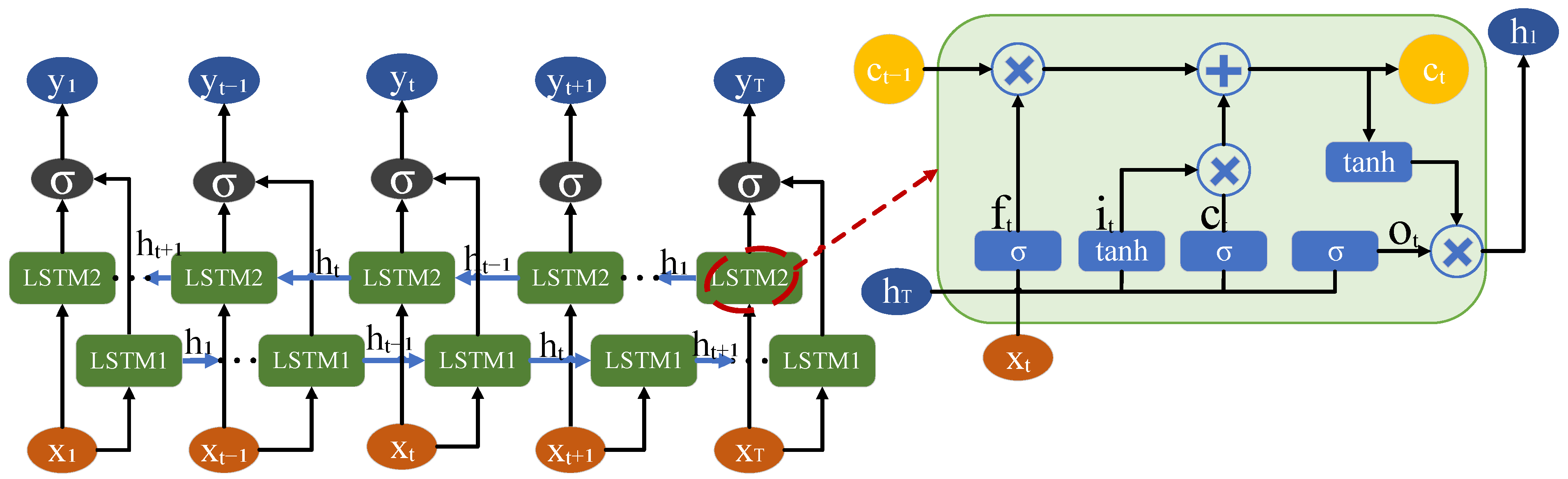
2.3.3. Temporal Feature Extraction in Tool Wear Monitoring

In tool wear state monitoring, the bidirectional LSTM network serves as a powerful model for processing sequential data, effectively capturing bidirectional temporal information of the tool during processing. Since tool wear is a cumulative process, vibration signals and other sensor data often exhibit strong temporal dependencies. Unidirectional temporal sequence models (e.g., standard LSTM) can only capture signal features from one direction and cannot fully reflect the global dynamic characteristics of tool wear. BiLSTM utilizes both forward and backward information flows, further enhancing the modeling capability for long sequential signals, demonstrating stronger adaptability in complex industrial applications.

As shown in Figure 7, the input at each time step t, $x_t$ is fed into two LSTM networks, including a forward LSTM (from left to right) and a backward LSTM (from right to left). The forward LSTM processes information before time step t while the backward LSTM processes information after time step t. At each time step, the forward LSTM and backward LSTM generate their respective hidden states ${\overrightarrow{h}}_t$ and ${\overrightarrow{h}}_t$. The detailed structure of the LSTM unit is shown on the right side of the figure, where it can be observed that the LSTM controls the flow and update of information through the introduction of the forget gate, input gate, candidate memory cell, and output gate. The specific calculations are as follows:

The forget gate $f_t$ controls which information from the memory cell $c_{t-1}$ needs to be retained at the current time step.

$$f_t=\sigma \left(W_f\cdot \left[h_{t-1},x_t\right]+b_f\right)$$

(6)

The input gate $i_t$ controls how the input $x_t$ at the current time step affects the memory cell.

$$i_t=\sigma \left(W_i\cdot \left[h_{t-1},x_t\right]+b_i\right)$$

(7)

The candidate memory cell ${\tilde{c}}_t$ generates the candidate content for the memory cell at the current time step.

$${\tilde{C}}_t=\tan \mathrm{h}\left(W_c\cdot \left[h_{t-1},x_t\right]+b_c\right)$$

(8)

The memory cell update $c_t$ is determined by the combined effect of the forget gate and input gate, deciding the update of the memory content.

$$C_t=f_t\cdot C_{t-1}+i_t\cdot {\tilde{C}}_t$$

(9)

The output gate $o_t$ controls the output from the hidden state $h_t$.

$$o_t=\sigma \left(W_o\cdot \left[h_{t-1},x_t\right]+b_o\right)$$

(10)

The hidden state update uses the memory cell $c_t$ to update the hidden state at time step t.

$$h_t=o_t\cdot \tan \mathrm{h}\left(C_t\right)$$

(11)

In the BiLSTM model depicted in the figure, the forward and backward hidden states at each time step are concatenated, resulting in a unified output that encapsulates information from both temporal directions.

$$H_t=\left[\overrightarrow{h_t},\overleftarrow{h_t}\right]$$

(12)

In summary, the bidirectional LSTM simultaneously considers the information before and after the input sequence, allowing the model to better capture the global features of the signal during the tool wear process. This approach is more suitable for complex tasks requiring sequential relationship modeling. Through this method, the prediction of the tool wear state can be made more accurate and robust, which in turn extends the lifespan of the tool, improving processing efficiency. In practical applications, the BiLSTM model not only captures the current wear state of the tool but also predicts future wear trends, providing reliable data for decision making.

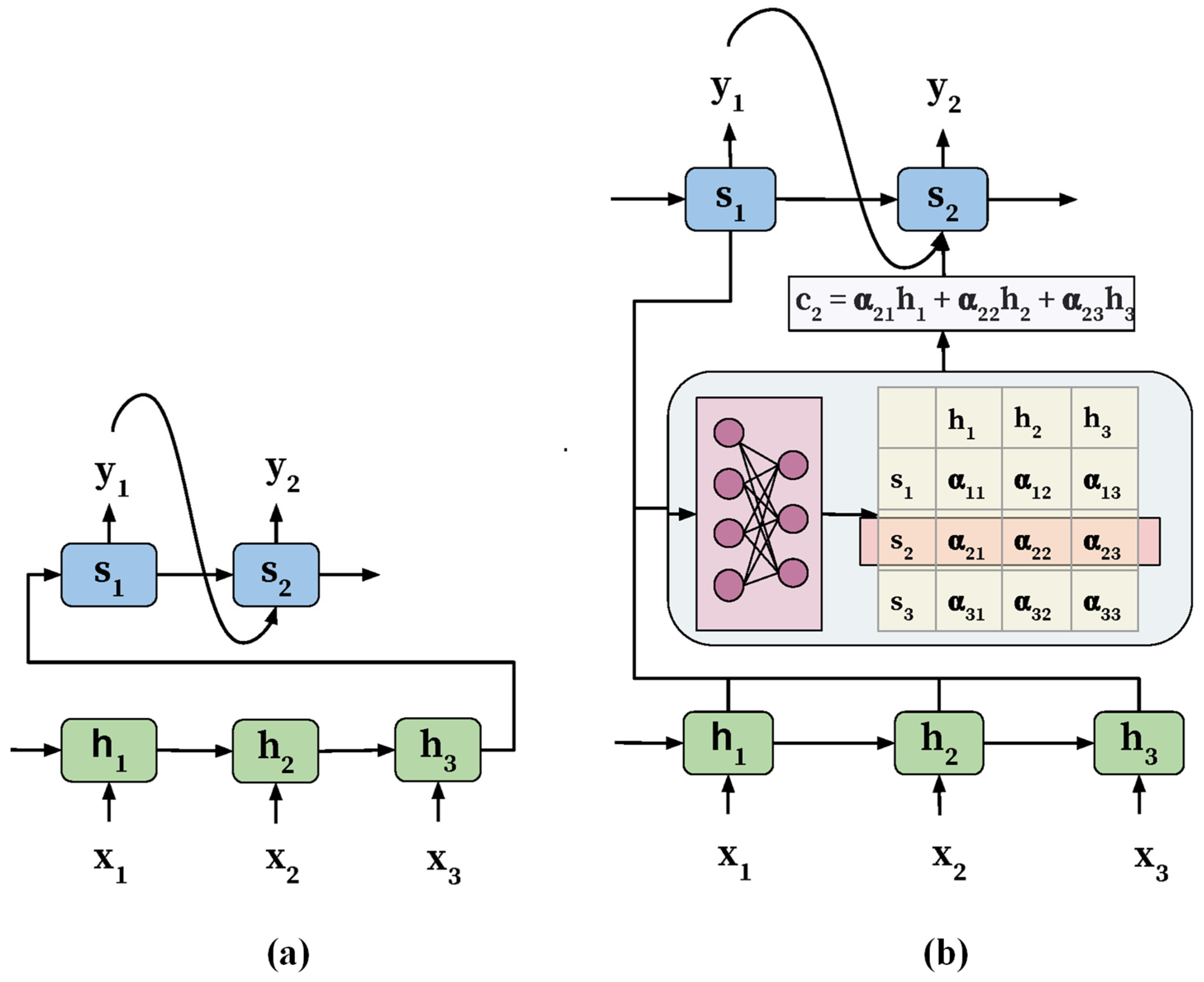
2.3.4. Introduction of AM

Combining the AM with the BiLSTM network in tool life prediction tasks can significantly enhance model performance. Specifically, the AM calculates the relative importance of each time step in the input sequence, effectively capturing long-term dependencies and optimizing tool wear state predictions. The combination of self-attention mechanisms with BiLSTM networks can simultaneously capture forward and backward temporal features and focus on important time steps through weight allocation.

Figure 8a shows the structure of a standard sequence model, where each hidden state $h_t$ depends on the input sequence $x_t$ and is sequentially passed to subsequent time steps. However, solely relying on the LSTM network may overlook critical information from certain time steps due to distant inputs or noise interference. Part (b) incorporates the AM, demonstrating how different weights are assigned to different time steps to enhance the model’s predictive ability. In the AM, the hidden state $h_t$ is compared with the hidden states of previous time steps, and attention weights ${\alpha }_{ti}$ are calculated based on this comparison. These weights are used to compute a weighted sum of the hidden states, resulting in the final context vector $c_t$. The calculation is as follows:

$$c_t={\displaystyle \sum _{i=1}^T{\alpha }_{ti}}{h}_i$$

(13)

where ${\alpha }_{ti}$ is the attention weight between time step t and time step i, computed as follows:

$${\alpha }_{ti}={\displaystyle \frac{\exp \left(e_{ti}\right)}{{\displaystyle \sum _{k=1}^T\exp }\left(e_{tk}\right)}}$$

(14)

where $e_{ti}$ represents the alignment score (or relevance) between time step t and time step i, which is usually computed through a neural network that takes previous hidden states as input. In Figure 8b, the AM allows the model to compute output $s_t$, which not only relies on the corresponding hidden state $h_t$ at the current time step but also integrates information from all hidden states of the entire sequence, effectively capturing global dependencies between different time steps. This global dependency is crucial for accurately predicting tool wear states, as vibration signals and other data often exhibit long-term dependencies and nonlinearities. The model needs to handle information from distant time steps to improve prediction accuracy. Through the use of the AM, the model can better capture both short-term and long-term dependencies in the sequence, leading to improved prediction precision. This framework, combined with BiLSTM, makes the model more accurate and reliable, especially in complex industrial environments, where the ability to predict tool wear and remaining tool life is critical.

2.3.5. TTAO Optimization Algorithm for Multi-Scale Temporal Feature Extraction and Monitoring of Tool Wear

The WPT, through multi-scale decomposition of vibration signals, can effectively capture features across different frequency bands during the tool wear process. On the other hand, BiLSTM demonstrates clear advantages in handling sequential data. By combining forward and backward information, the bidirectional LSTM enables the model to simultaneously consider both past and future time steps, thereby improving the recognition of wear state changes. However, relying solely on the WPT and BiLSTM is insufficient to fully address the complexity and non-stationarity present in vibration signals. To extract key features and construct a robust and efficient recognition model, this paper introduces the TTAO algorithm. An innovative method for tool wear state monitoring is proposed through the integration of BiLSTM and WPT. TTAO optimizes the model training process by simulating a triangular topology structure. In the early stages, it performs extensive exploration by randomly generating several vertices as candidate solutions. As iterations progress, these candidate solutions are incrementally optimized, helping the algorithm avoid local optima. The alternating phases of exploration and exploitation allow TTAO not only to swiftly identify feasible solutions but also to progressively adjust the step size, converging towards a global optimum. This hybrid approach ensures the development of a more accurate and reliable model for monitoring tool wear.

In the initial stage of the experiment, the TTAO algorithm first generates an initial population for the initial configuration of model hyperparameters. Each individual in the population represents a different parameter combination, including parameters such as learning rate and number of hidden nodes in the BiLSTM, generated using the following formula:

$$X_{1i}=LB+\left(UB-LB\right)\times rand\left(0,1\right)$$

(15)

where UB and LB are the upper and lower bounds of the search space, respectively. In this step, an initial set of solutions is generated, representing multiple possible parameter settings for the model in the search space. Then, individuals from the initial population are further used to generate the second and third groups of individuals, which are calculated according to Equations (16) and (17):

$$X_{2i}=X_{1i}+l\times f\left(\theta \right)$$

(16)

$$X_{3i}=X_{1i}+l\times f\left(\theta +{\displaystyle \frac{\pi }{3}}\right)$$

(17)

In the above equations, l represents the size of the triangular topology unit. Its value gradually decreases with the increase in iteration number, indicating that as the iteration progresses, the search region narrows from broad exploration to localized exploitation. The updated formula is expressed as follows:

$$l=9\times e^{{\displaystyle \frac{-t}{T}}}\mathrm{tag}18$$

(18)

In this equation, t is the current iteration number and T is the total number of iterations. This formula shows that l decreases as the number of iterations increases. Functions $f\left(\theta \right)$ and $f\left(\theta +{\displaystyle \frac{\pi }{3}}\right)$ are two directional vectors, which are computed as follows:

$$f\left(\theta \right)=\left(\cos \left({\theta }_1\right),\cos \left({\theta }_2\right),\mathrm{dots},\cos \left({\theta }_D\right)\right)$$

(19)

$$f\left(\theta +{\displaystyle \frac{\pi }{3}}\right)=\left(\cos \left({\theta }_1+{\displaystyle \frac{\pi }{3}}\right),\cos \left({\theta }_2+{\displaystyle \frac{\pi }{3}}\right),\mathrm{dots},\cos \left({\theta }_D+{\displaystyle \frac{\pi }{3}}\right)\right)$$

(20)

Here, ${\theta }_j$ j = 1,2,…,D is a random number between [0, π]. After generating the initial population, TTAO computes the directional vectors dir1 and dir2 to guide the population towards better solutions. The corresponding formulas (22) and (23) are expressed as follows:

$$dir1=X_{best}-X^{\left(1\right)}$$

(21)

$$dir2=X_{best}-X^{\left(2\right)}$$

(22)

where $X_{best}$ represents the best-performing individual in the current iteration, and $X_{rand}$ is a randomly selected population individual. Through the calculation of these directional vectors, the individuals in the population can more effectively approach the global optimal solution. In the aggregation phase, the three groups of individuals generated in the previous steps are aggregated into new candidate solutions, which are calculated as follows:

$$X_{4i}=r_1\times X_{1i}+r_2\times X_{2i}+r_3\times X_{3i}$$

(23)

where $r_1$, $r_2$, and $r_3$ are random numbers in the range [0, 1], and ${\displaystyle \sum _{i=1}^3{r}_i}=1$. Through this aggregation operation, the TTAO algorithm generates new candidate solutions, further enhancing the diversity and robustness of the solution set. Next, TTAO simulates the crossover operation of genetic algorithms, generating new individuals through the linear combination of the best and randomly selected individuals, as follows:

$$X_{ni}=r_4\times X_b+r_5\times X_r$$

(24)

where $X_r$ is a randomly selected individual from the population, $X_b$ is the current best individual, and $r_4$ and $r_5$ are random numbers. At this stage, the newly generated individuals enhance the diversity of the population through linear combination. The fitness values of the new individuals are then updated by comparing their performance with the current best and second-best individuals. Equations (25) and (26) are used to update the fitness values. TTAO adjusts the population based on these fitness values and retains the best-performing individuals:

$$X_{bi}=\left\{\begin{array}{l}{X}_{ni}\hspace{1em}\mathrm{if}{f}_{ni}<f_{bi}\hfill \\ X_{bi}\hspace{1em}\mathrm{otherwise}\hfill \end{array}\right.$$

(25)

$$X_{sbi}=\left\{\begin{array}{l}{X}_{ni}\hspace{1em}\hspace{0.17em}\mathrm{if}{f}_{sni}<f_{sbi}\hfill \\ X_{sbi}\hspace{1em}\mathrm{otherwise}\hfill \end{array}\right.$$

(26)

During the development phase, TTAO performs a local search based on the current best and second-best solutions to generate new solutions. This phase is computed using the following formula:

$$X_{n2i}=X_{bi}+\alpha \left(X_{bi}-X_{sbi}\right)$$

(27)

where α is the size of the aggregation range, updated as follows:

$$\alpha =\ln \left({\displaystyle \frac{e^{\frac{3}{T}\left(1-\frac{t}{T}+e^3\right)}}{e^{\frac{3}{T}}}}\right)$$

(28)

Finally, the newly generated solutions are compared with the current best solution, and the individual with a higher fitness value replaces the current best solution, ensuring that the result of each iteration gradually approaches the global optimal solution:

$$X_{bi}=\left\{\begin{array}{l}{X}_{n2i}\hspace{1em}\mathrm{if}{f}_{n2i}<f_{\mathrm{bi}}\hfill \\ X_{bi}\hspace{1em}\hspace{0.17em}\hspace{0.17em}\mathrm{otherwise}\hfill \end{array}\right.$$

(29)

Through these steps, the TTAO algorithm effectively utilizes the triangular topology structure for optimization, progressively approaching the global optimal solution.

The introduction of the triangular topology adaptive optimization (TTAO) algorithm significantly enhances the performance of the titanium alloy tool wear monitoring system. First, the TTAO algorithm optimizes the selection of model hyperparameters, enabling the neural network model to learn more efficiently and preventing the overfitting issues commonly encountered in traditional methods. Through its unique triangular topology structure, TTAO enhances the global search capability of the model, effectively avoiding the risk of getting trapped in local optima. Additionally, by iteratively updating the population individuals, TTAO gradually narrows the search space, significantly improving the model’s convergence speed and accelerating the training process.

By optimizing the key parameters of the BiLSTM and WPT models, TTAO ensures that the model can accurately extract deep-level features from complex, non-stationary signals. Furthermore, the optimization process of TTAO improves the model’s ability to handle the extraction of multi-scale features from vibration signals. In tool wear state prediction, the multi-band characteristics of vibration signals are crucial for accurately identifying the wear state. By incorporating the WPT for multi-scale decomposition of vibration signals, TTAO ensures more precise feature extraction across different frequency bands, thereby enhancing the ability to recognize wear states. The introduction of the BiLSTM model strengthens the handling of sequential data, allowing the model to fully leverage both the forward and backward temporal features of the signal, further improving the accuracy of wear prediction.

The incorporation of the TTAO optimization algorithm makes the tool wear monitoring system more efficient and accurate when dealing with complex operating conditions. By optimizing model parameters, TTAO improves the overall robustness of the system, not only enhancing the accuracy of wear state predictions but also accelerating the model’s training speed. This greatly optimizes parameter selection and learning performance in vibration signal processing.

Figure 9 illustrates the complete process of the tool wear monitoring method based on the combination of the TTAO optimization algorithm and the AM-BiLSTM network. The entire process can be divided into two main stages: the training phase and the testing phase.

In the training phase, the first step is dataset preparation, starting with the collection of the dataset, which includes vibration signals and other relevant information. The data are split into two parts: the training set and the testing set. Before training begins, it is necessary to set the parameters for the TTAO algorithm, such as population size and the number of iterations, which provide the necessary initial conditions for the optimization process. Then, TTAO generates a set of random initial solutions, referred to as random population generation, representing the initial configurations of the neural network. After the random population is generated, the AM-BiLSTM model is trained using the training set. The model incorporates an AM within the BiLSTM structure. Through bidirectional LSTM, the model captures both forward and backward temporal features in the vibration signals, while the AM highlights important time steps. Once the model training is completed, the fitness of each network configuration is computed. The fitness calculation evaluates the performance of the model under the given configuration, where the fitness score directly reflects the accuracy of the model in predicting tool wear states.

Next, the core part of the TTAO algorithm begins—iterative optimization. By updating population X, the TTAO algorithm adjusts the population configuration using adaptive step sizes and triangular topology structures to continuously search for better solutions. After each iteration, TTAO selects the best solution based on fitness and checks whether the stop condition has been met, such as reaching the maximum number of iterations or achieving the desired model performance. If the condition is not met, the process loops, continuing to optimize the population and retrain the model. If the condition is satisfied, the loop terminates, and the best network configuration is saved.

In the testing phase, after the training phase has concluded, the TTAO algorithm determines the best configuration, which represents the optimal network parameters found through iterative optimization. Based on this configuration, the testing set is used to predict the tool wear state with the optimized model. Finally, in the performance evaluation step, the model’s performance on the testing set is assessed, mainly through metrics such as accuracy and F1 score, to measure the model’s ability to recognize tool wear states. If the evaluation results meet the expected targets, the entire process ends successfully. Through the combination of this optimization algorithm and the neural network model, the tool wear monitoring system not only improves recognition accuracy but also accelerates both the training and testing phases, ensuring the efficiency and reliability of the monitoring system.

3. Results and Discussion

3.1. Model Training

To ensure a thorough evaluation of the model’s performance, various metrics are employed to capture both qualitative and quantitative aspects of its predictive capabilities. These metrics provide a detailed understanding of how well the model generalizes to new data and how effectively it predicts tool wear. The following sections elaborate on the experimental results and the model’s evaluation based on these metrics.

3.1.1. Experimental Setup

To ensure the accuracy and consistency of the model training process, all experiments were conducted under the experimental environment configurations shown in

Table 2. Experimental Environment Configuration.

CPU	GPU	Deep Learning Framework	Operating System	Batch Size
12th Gen Intel(R) Core(TM) i5-12600KF 3.70 GHz	Nvidia GeForce RTX 4060	MATLAB R 2024a	Windows 11	64

. The model was built using MATLAB R2024a (MathWorks, Natick, MA, USA). The testing environment included a 12th Gen Intel Core i5-12600KF 3.70 GHz processor (Intel Corporation, Santa Clara, CA, USA), Nvidia GeForce RTX 4060 GPU (Nvidia Corporation, Santa Clara, CA, USA), and Windows 11 64-bit operating system (Microsoft Corporation, Redmond, WA, USA).

3.1.2. Evaluation Metrics

To validate the performance of the proposed TTAO-CNN-BiLSTM-AM model in tool wear prediction, this paper conducted a comprehensive analysis and verification using various evaluation metrics. The specific evaluation metrics included test set prediction comparison graphs, confusion matrices, ROC curves, and model convergence curves. These evaluation methods showcase the model’s performance from different perspectives.

The test set prediction comparison graph is used to show the difference between the model’s predicted values and the true values. Through this graph, one can visually observe the model’s fitting performance on the test set. If the model’s prediction results are basically consistent with the true values, it indicates that the model has high prediction accuracy. To quantitatively measure the model’s prediction accuracy, this paper uses the mean squared error (MSE). The MSE calculates the error between the model’s predicted values and the true values, with lower MSE values indicating higher prediction accuracy. The MSE calculates the error between the model’s predicted values and the true values, and its formula is as follows:

$$MSE={\displaystyle \frac{1}{n}}{\displaystyle \sum _{i=1}^n{\left({\widehat{y}}_i-y_i\right)}^2}$$

(30)

where ${\widehat{y}}_i$ represents the model’s predicted value, $y_i$ represents the true value, and $n$ is the number of test samples. The lower the MSE value, the smaller the error between the model’s predicted values and the true values, and the higher the model’s prediction accuracy. The confusion matrix is used to display the relationship between the model’s prediction results and the actual results, which can reflect the model’s classification performance in detail. Based on the confusion matrix, the following common evaluation metrics can be defined:

Accuracy: Represents the proportion of correctly predicted samples to the total number of samples, calculated as follows:

$$Accuracy={\displaystyle \frac{TP+TN}{TP+TN+FP+FN}}$$

(31)

where $TP$ is true positive, $TN$ is true negative, $FP$ is false positive, and $FN$ is false negative. Through the confusion matrix, one can effectively evaluate the model’s classification performance across different categories and quantify the types of classification errors, such as false positives ($FP$) and false negatives ($FN$). The ROC curve is used to measure the model’s classification performance under different thresholds. By plotting the relationship between the true positive rate (TPR) and the false positive rate (FPR), the ROC curve demonstrates the model’s classification ability. The calculation formulas are as follows:

TPR, also known as sensitivity:

$$TPR={\displaystyle \frac{TP}{TP+FN}}$$

(32)

FPR:

$$FPR={\displaystyle \frac{FP}{FP+TN}}$$

(33)

AUC (area under the curve): The area under the ROC curve measures the overall classification performance of the model; the closer the AUC value is to 1, the better the model’s performance. The model convergence curve shows the changes in the loss function during the training process. This paper uses the mean squared error as the loss function to measure the training effect of the model. By plotting the curve of the loss function against the number of iterations, one can observe whether the model converges. When the curve gradually tends to be stable and the loss value is low, it indicates that the model has converged and achieved a good training effect.

3.2. Experimental Results and Analysis

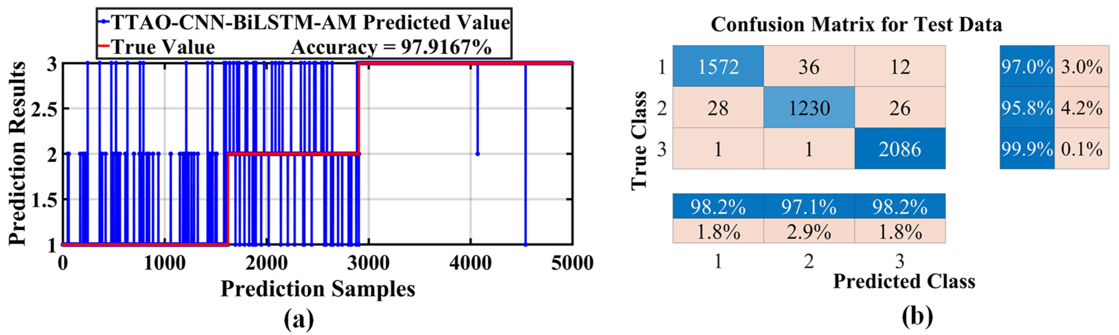
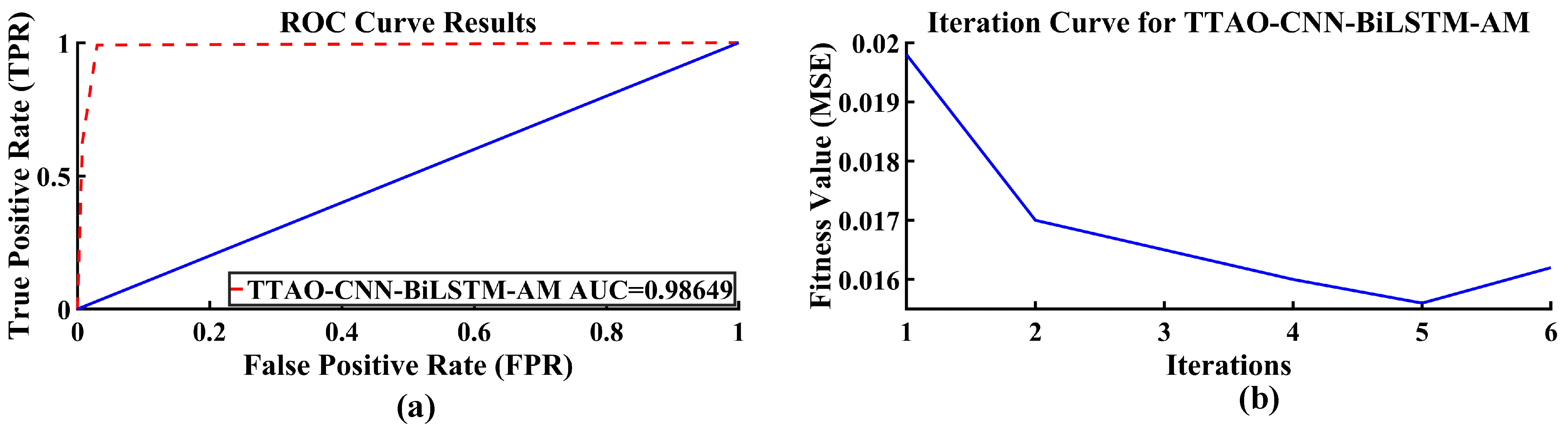
3.2.1. Model Experimental Results

Figure 10a displays the test set prediction comparison graph, comparing the match between the model’s predicted values and the true values in the test set. From the figure, it can be seen that the model’s predicted values are basically consistent with the true values. Especially on most sample points, the model can accurately predict the wear state. The average accuracy of the test set is 97.9167%, further verifying the model’s robustness and accuracy. Although there are a few samples where the prediction results have some deviation from the true values, overall, the model still exhibits excellent prediction performance. The TTAO-CNN-BiLSTM-AM model successfully achieves high-precision prediction by effectively classifying samples with different wear states.

Figure 10b displays the confusion matrix of the TTAO-CNN-BiLSTM-AM model on the test set. The confusion matrix intuitively shows the model’s classification accuracy across different categories. For Category 1, 1572 samples were correctly classified, with a misclassification rate of 3.8%; for Category 2, the number of correctly classified samples was 1230, with a misclassification rate of 2.9%; for Category 3, 2086 samples were correctly classified, and almost all samples of Category 3 were correctly classified, with a classification accuracy of 99.9%. Overall, the model exhibits high accuracy in predicting the three wear states, with minimal errors, especially with almost no errors in recognizing Category 3. This further demonstrates the strong classification ability of the TTAO-CNN-BiLSTM-AM model in wear state prediction.

Figure 11a illustrates the ROC (receiver operating characteristic) curve of the TTAO-CNN-BiLSTM-AM model. This curve reflects the model’s classification performance under different thresholds. Observing the ROC curve reveals that the model’s TPR remains at a high level in most cases, while the FPR stays at a low level. The model’s AUC value reaches 0.98649, indicating that the model has extremely high classification ability. An AUC close to 1 means that the model’s predictive ability is very strong and can accurately distinguish between wear state and non-wear state data.

Figure 11b illustrates the convergence curve of the TTAO-CNN-BiLSTM-AM model during the optimization process. In this study, the proposed model achieves an MSE value of 0.0155, which is significantly lower than traditional models such as BP. This low MSE demonstrates the model’s ability to effectively minimize prediction errors and highlights its accuracy in predicting tool wear states. The observed curve shows that after the first iteration, the MSE value decreases rapidly, stabilizes gradually, and eventually converges around 0.0155. This reduction in the MSE reflects the model’s robustness in handling complex nonlinear data and emphasizes its potential to improve the sustainability of machining processes by reducing tool waste and increasing machining efficiency. Moreover, the introduction of the TTAO algorithm significantly accelerates the convergence speed. After only six iterations, the model reaches an optimal minimum fitness value, indicating that the TTAO algorithm efficiently optimizes the hyperparameters of the CNN and BiLSTM components. This ensures that the model identifies the optimal solution in a short time, enhancing both the efficiency and accuracy of the optimization process.

From the analysis of the above four figures, it can be concluded that the TTAO-CNN-BiLSTM-AM model proposed in this paper performs excellently in tool wear prediction. Whether from the ROC curve, confusion matrix, test set prediction comparison, or model convergence curve, the TTAO-CNN-BiLSTM-AM model exhibits strong classification and prediction abilities when dealing with complex nonlinear wear data. In addition, the TTAO algorithm significantly enhances the model’s optimization speed and convergence effect, making the entire training process more efficient and ensuring prediction accuracy. This model provides strong support for monitoring tool wear states.

3.2.2. Comparison of Detection Results from Different Models

The tool wear recognition model based on wavelet packet and TTAO-CNN-BiLSTM-AM proposed in this paper showed excellent performance in multiple experiments, verifying its superiority in handling complex nonlinear data. From

Table 3. Comparison of Detection Results from Different Models.

Model	Number of Feature Sets	Learning Rate	Average Accuracy (%)
BP	16,640	0.001	91.428
1D CNN	16,640	0.001	97.262
CNN-BiLSTM-AM	16,640	0.001	96.498
TTAO-CNN-BiLSTM-AM	16,640	0.001	98.649

, it can be seen that the TTAO-CNN-BiLSTM-AM model had the highest average accuracy, reaching 98.649%, far exceeding the traditional BP model (91.428%) and 1D CNN (97.262%). This result indicates that the TTAO optimization algorithm plays an important role in tool wear state recognition, significantly enhancing the model’s performance. Compared with ordinary deep learning models, TTAO further improves the model’s accuracy through optimized parameter selection and model learning processes. Although the CNN-BiLSTM-AM model performed well, achieving an accuracy of 96.498%, after combining with the TTAO algorithm, the model’s performance was significantly improved, indicating that TTAO has excellent optimization effects when dealing with complex nonlinear wear problems.

3.3. Discussion

The proposed tool wear state recognition model based on the WPT and TTAO-CNN-BiLSTM-AM demonstrates exceptional performance, which can be attributed to several key innovations, cost advantages, and optimization strategies. Compared to existing methods, this study achieves significant advancements in robustness, real-time performance, and cost-effectiveness.

The wavelet packet transform provides an effective means for extracting multi-scale features from vibration signals. Unlike traditional wavelet transforms, the WPT decomposes not only the low-frequency components but also further refines the high-frequency components, enabling more comprehensive capture of signal characteristics across various frequency bands. By utilizing three-level WPT decomposition, the model effectively extracts spectral characteristics associated with different tool wear states, laying a robust foundation for accurate feature classification. By contrast, the method proposed by Zhang et al. [33], which combines time-series signals with adaptive gradients in meta-learning, faces challenges in handling small sample datasets and struggles with feature discrimination in multi-condition scenarios. Our approach, through the WPT, enhances the extraction of time-frequency features, demonstrating better generalization capability under limited data conditions.

Additionally, the integration of TTAO significantly enhances the model’s global optimization capability. TTAO, by simulating a triangular topology, effectively avoids the local optima issues often encountered in traditional optimization algorithms and accelerates the convergence process. The experimental results show that the TTAO-CNN-BiLSTM-AM model achieved an average accuracy of 98.649%, far surpassing traditional models such as BP and 1D CNN. The combination of global search and local exploitation in the TTAO strategy enables the model to achieve optimal performance in handling nonlinear, multidimensional tool wear problems, especially under complex working conditions. Compared to the dynamic milling force-based approach proposed by Ma et al. [34], our method not only improves prediction accuracy but also reduces computational costs, thus providing a more practical solution for real-world applications.

The integration of the BiLSTM network and the attention mechanism further enhances the model’s ability to capture temporal features from vibration signals. BiLSTM leverages both forward and backward information in the input sequence, effectively capturing the global dynamic characteristics of tool wear. The attention mechanism allows the model to adaptively focus on the most critical features for tool wear state recognition, improving both accuracy and generalization. The experimental results indicate that the BiLSTM combined with the attention mechanism not only enhances the model’s capability to capture long-term dependencies in the signal but also effectively prevents overfitting during training. Compared to digital twin-based methods proposed by Liu et al. [35], which rely on extensive resources for real-time anomaly detection, our model achieves similar predictive accuracy with significantly lower implementation costs.

Another advantage of the proposed method lies in its cost effectiveness. Unlike methods that rely on multi-sensor signal fusion, such as that by Wang et al. [36], our approach uses single-sensor vibration data, avoiding the complexity of signal fusion and ensuring efficient implementation. This not only reduces equipment and computational requirements but also provides a streamlined workflow for tool wear monitoring. Furthermore, our method achieves superior real-time performance by leveraging the fast convergence capabilities of TTAO and BiLSTM, outperforming ensemble-learning strategies like those of Abadia et al. [37], which may require significant computational resources and time.

Robustness is another key strength of the proposed method. By integrating the WPT, BiLSTM, and attention mechanism, the model effectively captures critical features from vibration signals, maintaining high accuracy under noisy and complex conditions. This robustness is particularly beneficial in dynamic operating environments where real-time predictions are crucial. Compared to the multi-source transfer learning approach proposed by Gao et al. [38], which requires extensive domain adaptation, our model achieves consistent performance across varying tool wear scenarios with a simpler, more efficient framework.

In summary, the WPT and TTAO-CNN-BiLSTM-AM model provides a robust, cost-effective, and real-time solution for tool wear monitoring. Its superior performance in accuracy, cost efficiency, and adaptability makes it a promising candidate for intelligent manufacturing applications, especially under diverse operating conditions.

4. Conclusions

This paper proposes a hybrid model based on the WPT and TTAO-CNN-BiLSTM-AM for tool wear state recognition in titanium alloy milling processes. By collecting vibration signals from the machine tool spindle and performing the WPT, multi-frequency band energy features are extracted as model inputs, effectively capturing the multi-scale features of tool wear. The combination of CNN and BiLSTM allows the model to learn complex spatial features and temporal relationships from vibration signals. The introduction of the AM further enhances the model’s ability to extract key features. The innovative application of the TTAO algorithm significantly optimizes the model’s training process, overcoming issues such as local optima and slow convergence in traditional neural networks, thereby improving the accuracy and efficiency of tool wear state recognition.

The experimental results show that the model achieved an average accuracy of 98.649% in tool wear state prediction, outperforming traditional BP networks and models using CNN or BiLSTM alone. Evaluation metrics such as confusion matrices and ROC curves indicate that the model exhibits excellent classification ability and robustness under complex working conditions, fully validating the effectiveness and superiority of the proposed method.

The TTAO-CNN-BiLSTM-AM model not only demonstrates high application value in tool wear monitoring but also provides new ideas and methods for solving other nonlinear, multidimensional fault diagnosis problems. With this model, real-time monitoring and dynamic adjustment of tool states can be realized during manufacturing processes, thereby extending tool life, improving processing quality and efficiency, and providing strong support for tool management in intelligent manufacturing. While this study has achieved significant advancements in tool wear monitoring, the experiments were conducted under fixed machining parameters and materials. Future research will aim to expand the applicability and robustness of the proposed method by focusing on several key areas. First, experiments will be conducted with diverse machining parameters, such as varying cutting speeds, feed rates, and cutting depths, as well as using different materials, such as aluminum alloys and composites, to validate the model’s adaptability under different conditions. Second, simulation studies will be integrated with real industrial scenarios to optimize the model’s real-time deployment and ensure its performance in practical industrial environments. Lastly, the potential application of this method will be extended to other areas of intelligent manufacturing, such as fault diagnosis and predictive maintenance, to further enhance production efficiency and improve equipment reliability.

References

1. Wang, Q.; Chen, X.; An, Q.; Chen, M.; Guo, H.; He, Y. Research on cutting performance and tool life improvement methods of titanium alloy ultra-high speed milling tools. J. Manuf. Process. 2024, 131, 38–51. [Google Scholar] [CrossRef]
2. Liu, G.; Zhang, D.; Yao, C. Investigation of the grain refinement mechanism in machining Ti-6Al-4V: Experiments and simulations. J. Manuf. Process. 2023, 94, 479–496. [Google Scholar] [CrossRef]
3. Cardoso, G.C.; Grandini, C.R.; Rau, J.V. Comprehensive review of PEO coatings on titanium alloys for biomedical implants. J. Mater. Res. Technol. 2024, 31, 311–328. [Google Scholar] [CrossRef]
4. Nasir, V.; Sassani, F. A review on deep learning in machining and tool monitoring: Methods, opportunities, and challenges. Int. J. Adv. Manuf. Technol. 2021, 115, 2683–2709. [Google Scholar] [CrossRef]
5. Guo, X.; Lee, C. Preliminary study of phase-shifting strobo-stereoscopy for cutting tool monitoring. J. Manuf. Process. 2021, 64, 1214–1222. [Google Scholar] [CrossRef]
6. Fong, K.M.; Wang, X.; Kamaruddin, S.; Ismadi, M.-Z. Investigation on universal tool wear measurement technique using image-based cross-correlation analysis. Measurement 2021, 169, 108489. [Google Scholar] [CrossRef]
7. Bergs, T.; Holst, C.; Gupta, P.; Augspurger, T. Digital image processing with deep learning for automated cutting tool wear detection. Procedia Manuf. 2020, 48, 947–958. [Google Scholar] [CrossRef]
8. Du, M.; Wang, P.; Wang, J.; Cheng, Z.; Wang, S. Intelligent Turning Tool Monitoring with Neural Network Adaptive Learning. Complexity 2019, 2019, 8431784. [Google Scholar] [CrossRef]
9. Rimpault, X.; Chatelain, J.-F.; Klemberg-Sapieha, J.; Balazinski, M. Tool wear and surface quality assessment of CFRP trimming using fractal analyses of the cutting force signals. CIRP J. Manuf. Sci. Technol. 2017, 16, 72–80. [Google Scholar] [CrossRef]
10. Tiwari, K.; Shaik, A.; Arunachalam, N. Tool wear prediction in end milling of Ti-6Al-4V through Kalman filter based fusion of texture features and cutting forces. Procedia Manuf. 2018, 26, 1459–1470. [Google Scholar] [CrossRef]
11. Klocke, F.; Döbbeler, B.; Pullen, T.; Bergs, T. Acoustic emission signal source separation for a flank wear estimation of drilling tools. Procedia CIRP 2019, 79, 57–62. [Google Scholar] [CrossRef]
12. Niaki, F.A.; Michel, M.; Mears, L. State of health monitoring in machining: Extended Kalman filter for tool wear assessment in turning of IN718 hard-to-machine alloy. J. Manuf. Process. 2016, 24, 361–369. [Google Scholar] [CrossRef]
13. Cao, X.-C.; Chen, B.-Q.; Yao, B.; He, W.-P. Combining translation-invariant wavelet frames and convolutional neural network for intelligent tool wear state identification. Comput. Ind. 2019, 106, 71–84. [Google Scholar] [CrossRef]
14. Upase, R.; Ambhore, N. Experimental investigation of tool wear using vibration signals: An ANN approach. Mater. Today Proc. 2020, 24 Pt 2, 1365–1375. [Google Scholar] [CrossRef]
15. Zhou, C.; Guo, K.; Sun, J. An integrated wireless vibration sensing tool holder for milling tool condition monitoring with singularity analysis. Measurement 2021, 174, 109038. [Google Scholar] [CrossRef]
16. Yangue, E.; Ye, Z.; Kan, C.; Liu, C. Integrated deep learning-based online layer-wise surface prediction of additive manufacturing. Manuf. Lett. 2023, 35, 760–769. [Google Scholar] [CrossRef]
17. Liu, C.; Wang, R.R.; Ho, I.; Kong, Z.J.; Williams, C.; Babu, S.; Joslin, C. Toward online layer-wise surface morphology measurement in additive manufacturing using a deep learning-based approach. J. Intell. Manuf. 2023, 34, 2673–2689. [Google Scholar] [CrossRef]
18. Gouarir, A.; Martínez-Arellano, G.; Terrazas, G.; Benardos, P.; Ratchev, S. In-process Tool Wear Prediction System Based on Machine Learning Techniques and Force Analysis. Procedia CIRP 2018, 77, 501–504. [Google Scholar] [CrossRef]
19. Wang, J.; Wang, P.; Gao, R.X. Enhanced particle filter for tool wear prediction. J. Manuf. Syst. 2015, 36, 35–45. [Google Scholar] [CrossRef]
20. Wang, J.; Yan, J.; Li, C.; Gao, R.X.; Zhao, R. Deep heterogeneous GRU model for predictive analytics in smart manufacturing: Application to tool wear prediction. Comput. Ind. 2019, 111, 1–14. [Google Scholar] [CrossRef]
21. Sun, H.; Zhang, J.; Mo, R.; Zhang, X. In-process tool condition forecasting based on a deep learning method. Robot. Comput.—Integr. Manuf. 2020, 64, 101924. [Google Scholar] [CrossRef]
22. Shi, C.; Luo, B.; He, S.; Li, K.; Liu, H.; Li, B. Tool Wear Prediction via Multidimensional Stacked Sparse Autoencoders with Feature Fusion. IEEE Trans. Ind. Inform. 2019, 16, 5150–5159. [Google Scholar] [CrossRef]
23. Sick, B. On-line and indirect tool wear monitoring in turning with artificial neural networks: A review of more than a decade of research. Mech. Syst. Signal Process. 2002, 16, 487–546. [Google Scholar] [CrossRef]
24. Zhu, K.; Wong, Y.S.; Hong, G.S. Wavelet analysis of sensor signals for tool condition monitoring: A review and some new results. Int. J. Mach. Tools Manuf. 2009, 49, 537–553. [Google Scholar] [CrossRef]
25. Liu, Q.; Liu, J.; Liu, X.; Ma, J.; Zhang, B. Based on domain adversarial neural network with multiple loss collaborative optimization for milling tool wear state monitoring under different machining conditions. Precis. Eng. 2024, 91, 692–706. [Google Scholar] [CrossRef]
26. Mishra, D.; Pattipati, K.R.; Bollas, G.M. Gaussian mixture model for tool condition monitoring. J. Manuf. Process. 2024, 131, 1001–1013. [Google Scholar] [CrossRef]
27. Liu, D.; Liu, Z.; Wang, B.; Song, Q.; Wang, H.; Zhang, L. Leveraging artificial intelligence for real-time indirect tool condition monitoring: From theoretical and technological progress to industrial applications. Int. J. Mach. Tools Manuf. 2024, 202, 104209. [Google Scholar] [CrossRef]
28. Hao, Y.; Zhu, L.; Wang, J.; Shu, X.; Yong, J.; Xie, Z.; Qin, S.; Pei, X.; Yan, T.; Qin, Q.; et al. Ball-end tool wear monitoring and multi-step forecasting with multi-modal information under variable cutting conditions. J. Manuf. Syst. 2024, 76, 234–258. [Google Scholar] [CrossRef]
29. Qiang, B.; Shi, K.; Ren, J.; Shi, Y. Multi-source online transfer learning based on hybrid physics-data model for cross-condition tool health monitoring. J. Manuf. Syst. 2024, 77, 1–17. [Google Scholar] [CrossRef]
30. Wen, D.L.W.; Soon, H.G.; Kumar, A.S. Micro-milling digital twin for real-time tool condition monitoring. Manuf. Lett. 2024, 41, 1231–1236. [Google Scholar] [CrossRef]
31. Zhao, S.; Zhang, T.; Cai, L.; Yang, R. Triangulation topology aggregation optimizer: A novel mathematics-based meta-heuristic algorithm for continuous optimization and engineering applications. Expert Syst. Appl. 2023, 238 Pt B, 121744. [Google Scholar] [CrossRef]
32. ISO-8688-1/1994; Cranes—Design Principles for Loads and Load Combinations—Part 1: General principles. ISO: Geneva, Switzerland, 2014.
33. Zhang, B.; Liu, X.; Yue, C.; Liang, S.Y.; Wang, L. Meta-learning-based approach for tool condition monitoring in multi-condition small sample scenarios. Mech. Syst. Signal Process. 2024, 216, 111444. [Google Scholar] [CrossRef]
34. Ma, J.; Zhang, Y.; Jiao, F.; Cui, X.; Zhang, D.; Ren, L.; Zhao, B.; Pang, X. Dynamic milling force model considering vibration and tool flank wear width for monitoring tool states in machining of Ti-6AI-4V. J. Manuf. Process. 2024, 124, 1519–1540. [Google Scholar] [CrossRef]
35. Liu, Z.; Lang, Z.-Q.; Gui, Y.; Zhu, Y.-P.; Laalej, H. Digital twin-based anomaly detection for real-time tool condition monitoring in machining. J. Manuf. Syst. 2024, 75, 163–173. [Google Scholar] [CrossRef]
36. Wang, H.; Wang, S.; Sun, W.; Xiang, J. Multi-sensor signal fusion for tool wear condition monitoring using denoising transformer auto-encoder Resnet. J. Manuf. Process. 2024, 124, 1054–1064. [Google Scholar] [CrossRef]
37. Abadia, J.J.P.; Zabaljauregui, M.C.; Barrenechea, F.L. A meta-learning strategy based on deep ensemble learning for tool condition monitoring of machining processes. Procedia CIRP 2024, 126, 429–434. [Google Scholar] [CrossRef]
38. Gao, Z.; Chen, N.; Yang, Y.; Li, L. An innovative multisource multibranch metric ensemble deep transfer learning algorithm for tool wear monitoring. Adv. Eng. Inform. 2024, 62, 102659. [Google Scholar] [CrossRef]
Figure 1. Tool wear monitoring and prediction workflow.
Processes 13 00013 g001
Figure 2. Tool milling vibration acquisition platform.
Processes 13 00013 g002
Figure 3. Time domain image of input signal. (a) Initial wear. (b) Normal wear. (c) Rapid wear.
Processes 13 00013 g003
Figure 4. Comparison between DWT and WPT for multilevel signal decomposition. (a) Multilevel decomposition structure of DWT. (b) Multilevel decomposition structure of WPT.
Processes 13 00013 g004
Figure 5. The wavelet packet 3rd layer signal spectrum. (a) Initial wear. (b) Normal wear. (c) Rapid wear.
Processes 13 00013 g005aProcesses 13 00013 g005b
Figure 6. The energy ratio of each band. (a) Initial wear. (b) Normal wear. (c) Rapid wear.
Processes 13 00013 g006
Figure 7. The BiLSTM structure.
Processes 13 00013 g007
Figure 8. Encoder–decoder architecture. (a) Traditional structure. (b) Attention mechanism-enhanced model structure.
Processes 13 00013 g008
Figure 9. Flowchart of the developed model.
Processes 13 00013 g009
Figure 10. Test results. (a) Prediction comparison graph. (b) Confusion matrix.
Processes 13 00013 g010
Figure 11. Test results. (a) The ROC curve. (b) The convergence curve.
Processes 13 00013 g011