
Machine Learning Algorithms That Emulate Controllers Based on Particle Swarm Optimization—An Application to a Photobioreactor for Algal Growth


Abstract
1. Introduction
- The PSO predictor predicts an optimal control value, but first, it searches for the optimal control sequence following its optimization mechanism using a swarm of particles and the PM. That is why it takes a relatively long time to find this value after a convergence process.
- The ML predictor (LR or RNN) predicts using an already-known regression function. Being an ML model, it reproduces what it has learned, the PSO predictor’s behavior. It does not search for anything. Moreover, it does not make numerical integrations of the PM. That is why it takes a much shorter time to calculate the predicted value.
- The ML predictor replaces the PSO predictor only in execution when the controller achieves the control action. Intrinsically, the solution is given by the PSO algorithm. The solutions are “learned” by the ML predictor; that is, the ML model emulates the PSO algorithm.
- What data are needed to capture the optimal (quasi-optimal) behavior of the couple (PSO and PM)?
- How are the data sets for the ML algorithms generated?
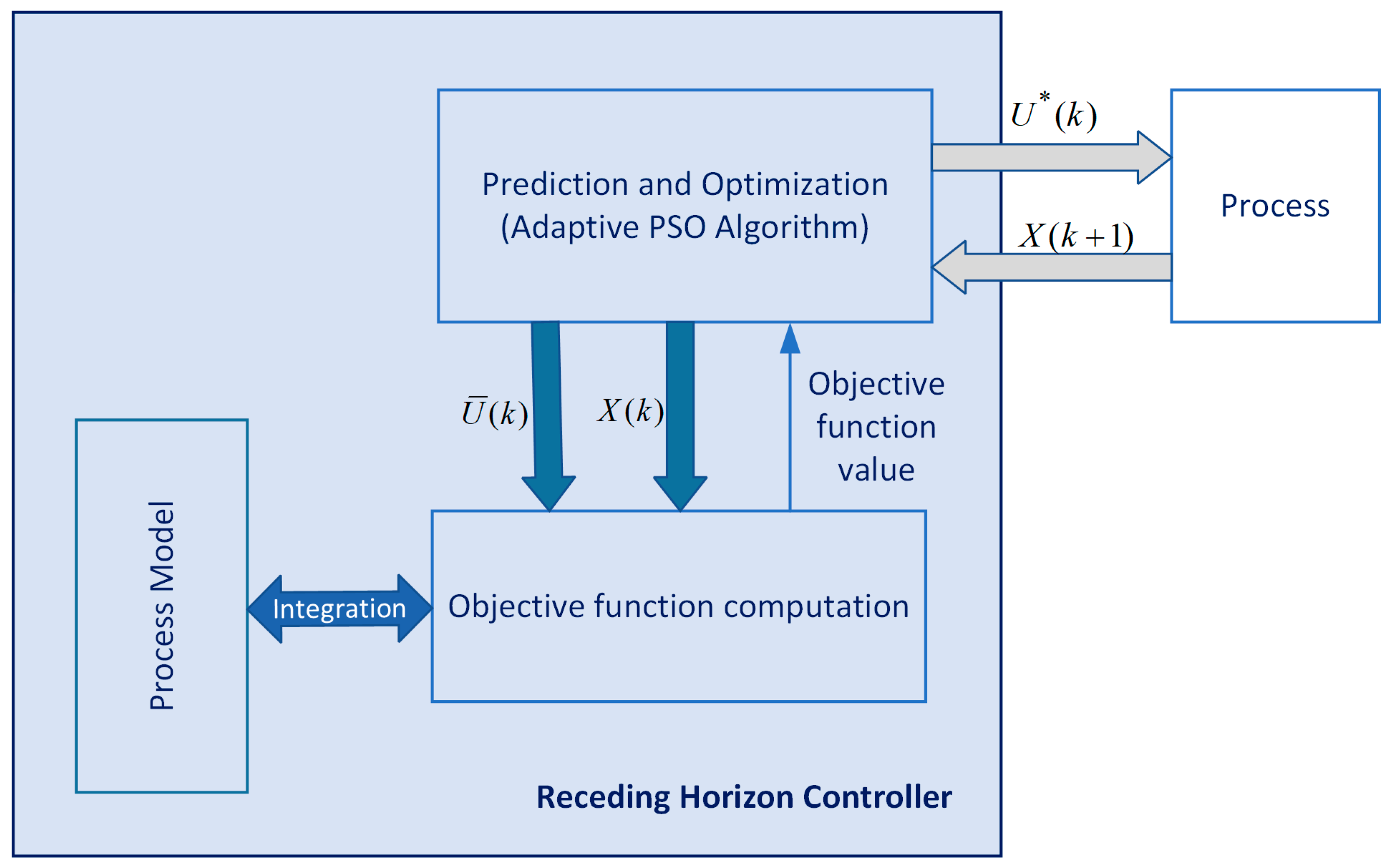
2. Controllers with Predictions Based on PSO: Connection with Machine Learning Algorithms
- The process model can include nonlinearities, imprecise, incomplete, and uncertain knowledge, correspond to a distributed-parameter system, etc.
- There are constraints, such as initial conditions, bound constraints, final constraints, etc.
- The cost function, which should be optimized, leads to a performance index.
- What does it mean that the ML algorithm must emulate the predictor?
- What data sets are used in training the ML, and how are they obtained?
- What kind of ML model can be used to achieve an appropriate controller?
3. Data Generation Using Closed-Loop Simulation over Control Horizon
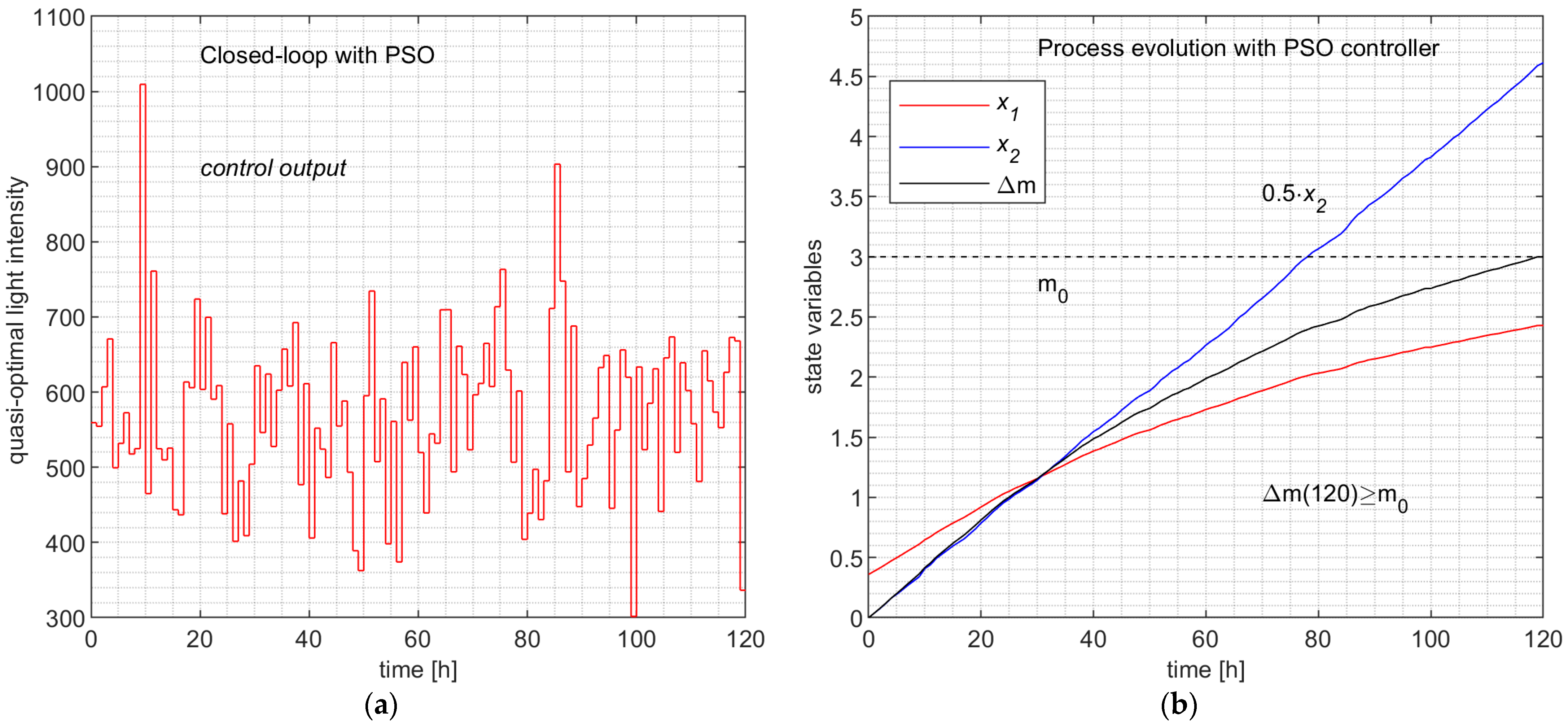
- The PSO has a stochastic character, and the convergence process is imperfect. So, the optimal control values are different (and so are the state vector’s values), even if the initial state is strictly the same.
- The initial state values are not the same. A standard initial state (of the standard batch) could be perturbed to simulate different initial conditions (the standard ones are imprecisely achieved).
4. The ML Controller: The Design Procedure and the General Algorithm
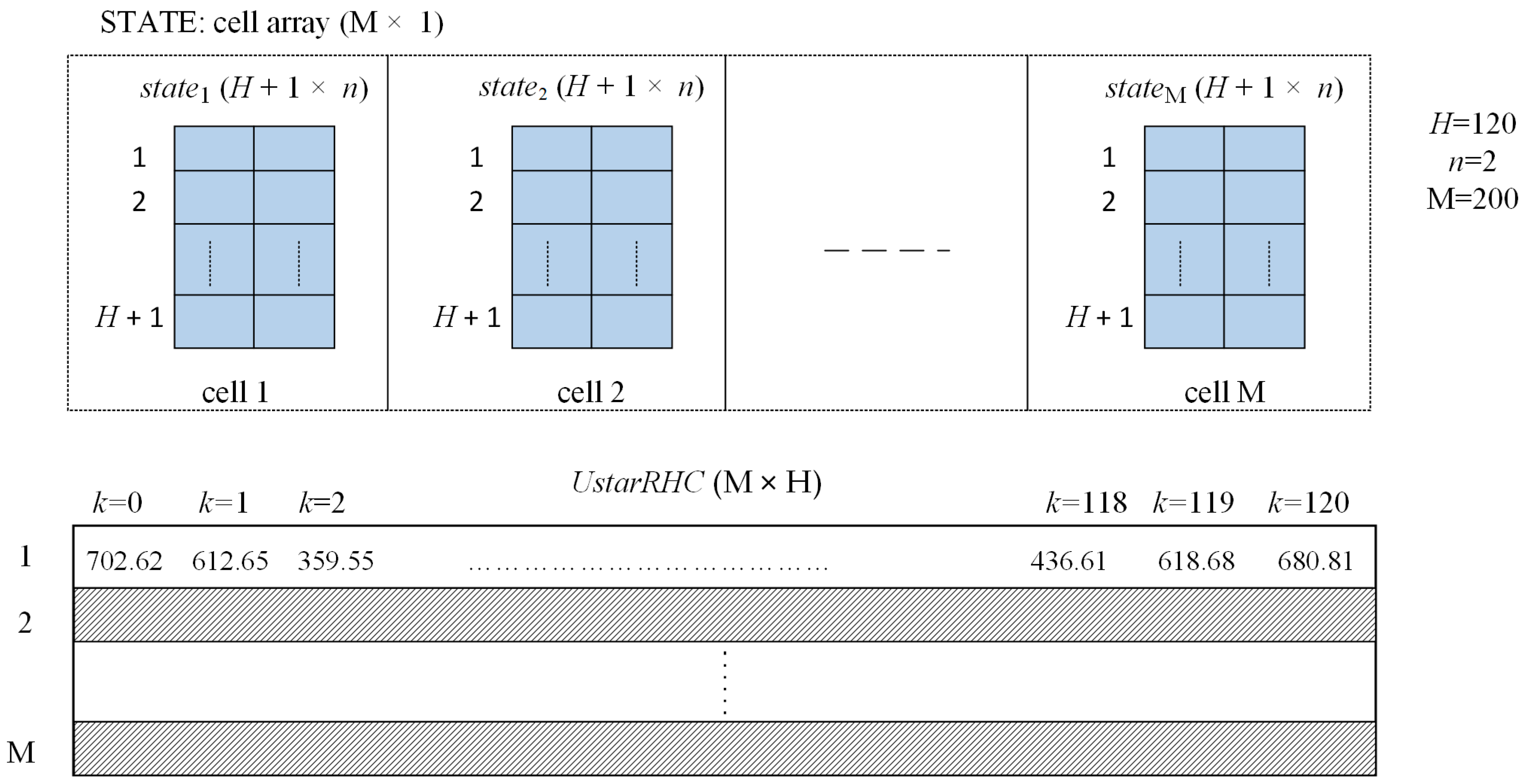
- The same PSO algorithm generates the M state inside a group.
- The M simulations work with the same PM.
- Each state , is transferred as the initial state to the predictor.
- The prediction horizon has sampling periods.
Design Procedure
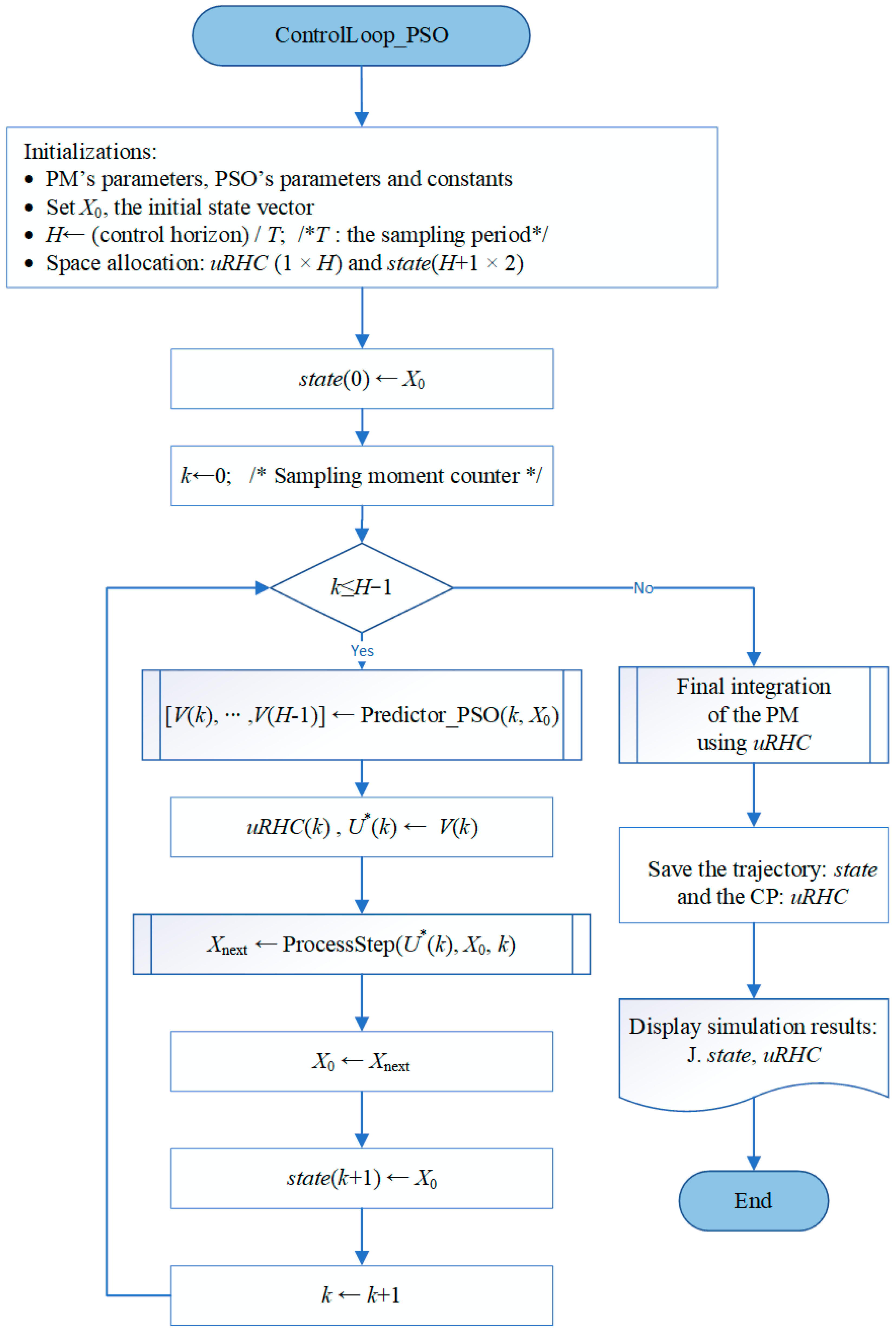
- Write the “ControlLoop_PSO” program simulating the closed-loop functioning of the controller based on the PSO algorithm over the control horizon. The output data are the quasi-optimal trajectory and its associated control profile ( and ).
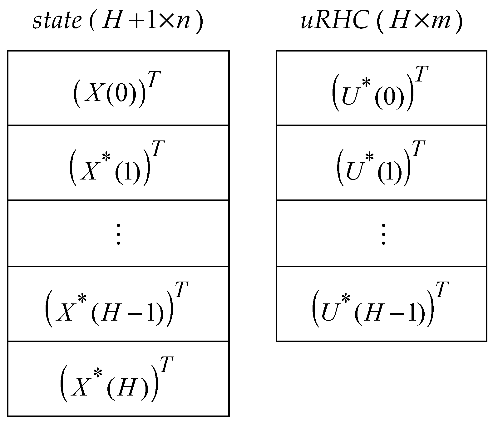
- Repeat M times the “ControlLoop_PSO” program’s execution to produce the sequences ( and ) and save them in data structures similar to those in Figure A1 (Appendix B).
- For each sampling period k, derive data sets similar to those in Table 1 from the data saved in step 2.
- Determine the set of functions using the data sets derived in step 3 and an ML model; a function is associated with each sampling period k.
- Implement the new controller based on the ML model, i.e., the set of functions determined in step 4.
- Write the “CONTROL_loop” program to simulate the closed-loop functioning equipped with the ML controller. The proposed method’s feasibility, performance index, solution quality, and execution time will be evaluated.
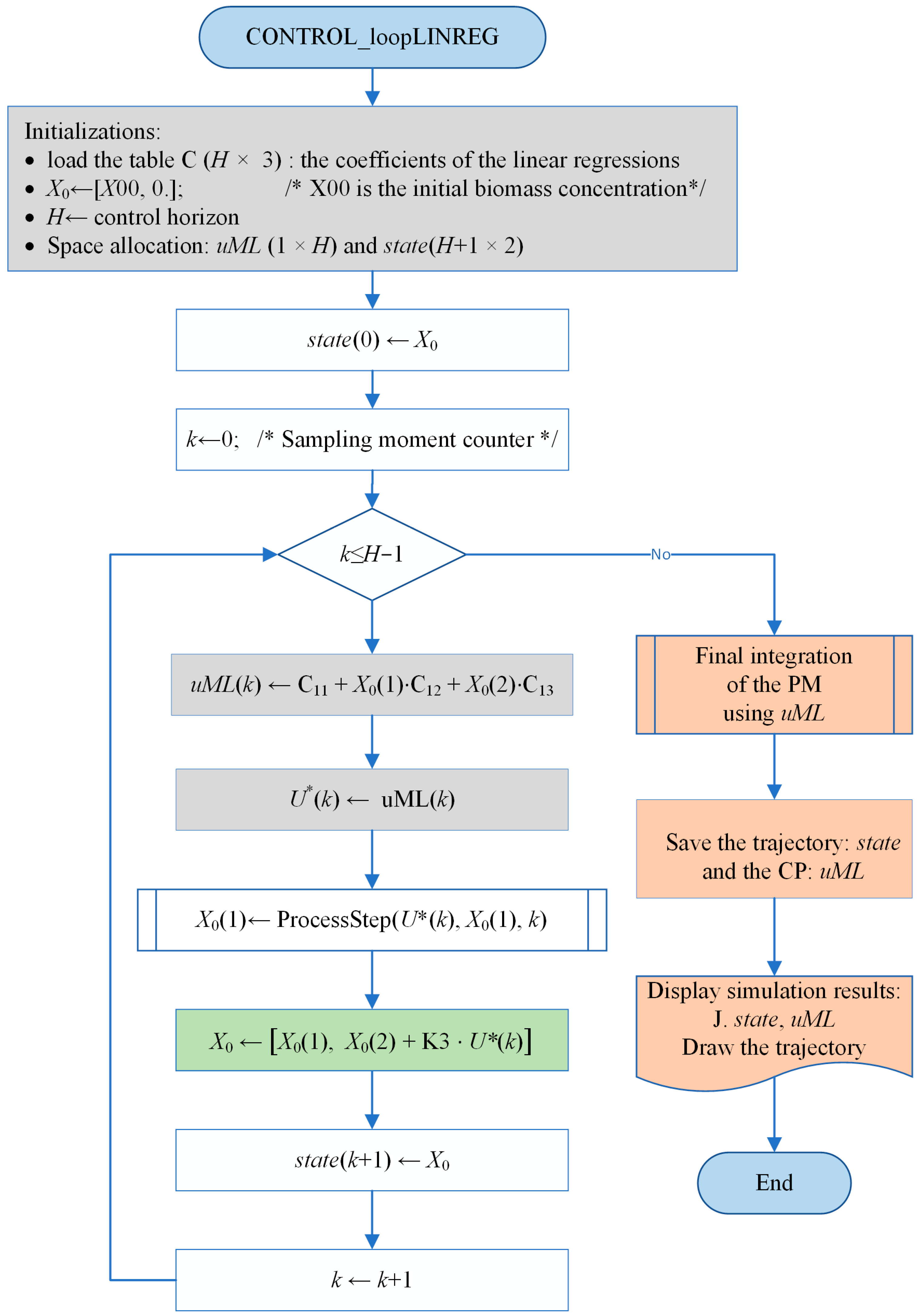
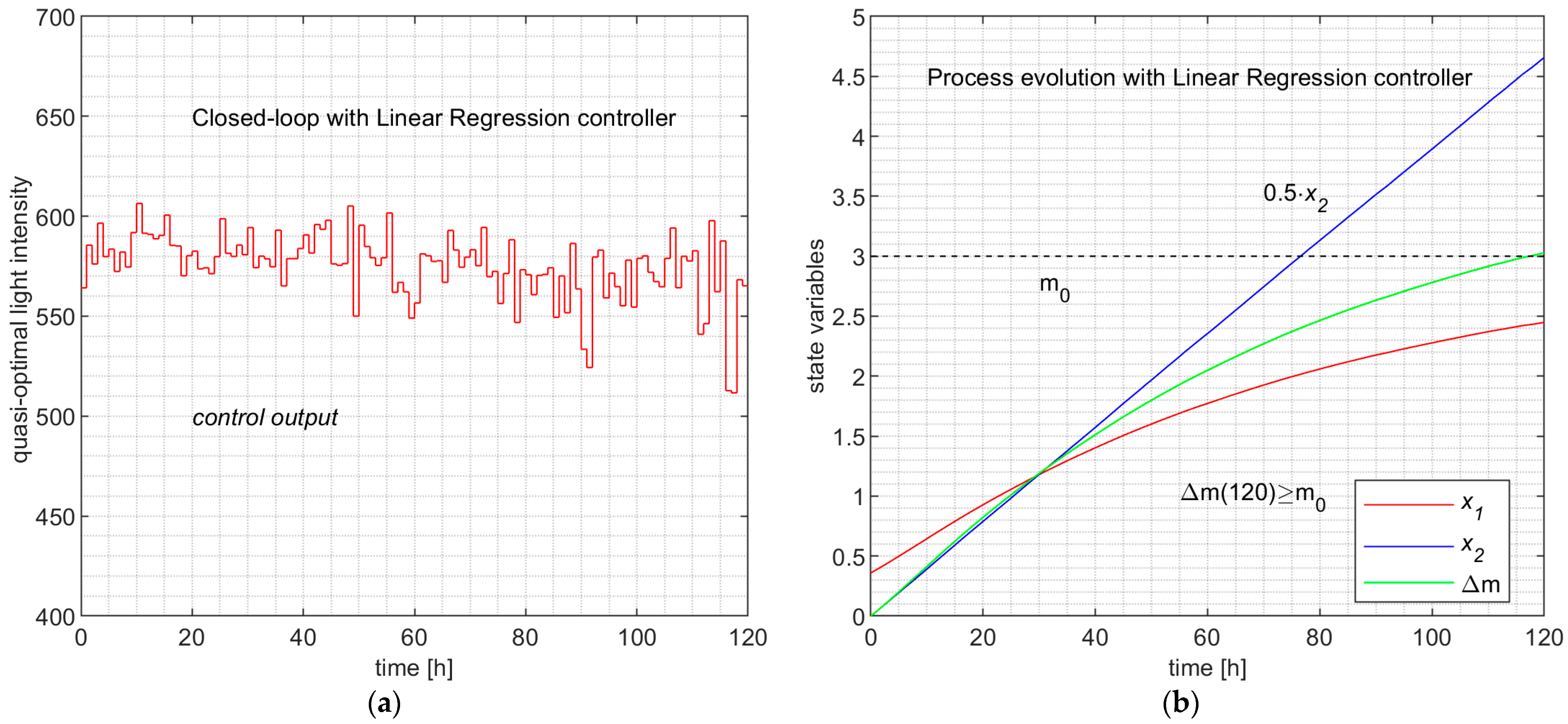
5. Linear Regression Controller
5.1. General Algorithm
5.2. Simulation Results
- The state variable has two elements.
- The coefficients’ matrix must be loaded from an existing file.
- The gray instructions make the predictions, avoiding any numerical integration.
- The green instruction updates the next state, which has two components. The amount of light irradiated in the current sampling period is added to x2(k).
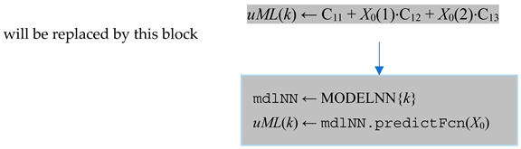
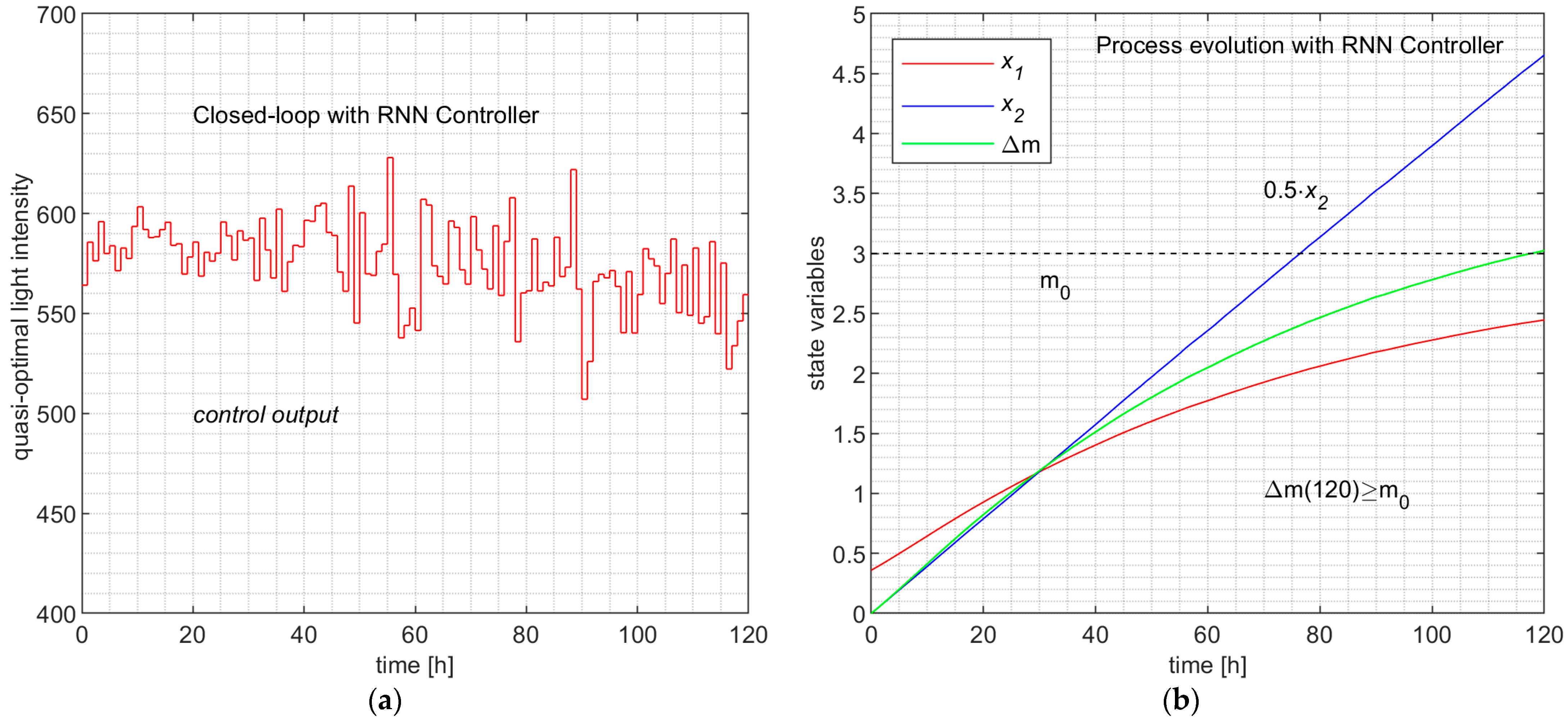
6. Controller Based on Regression Neural Networks
6.1. General Approach
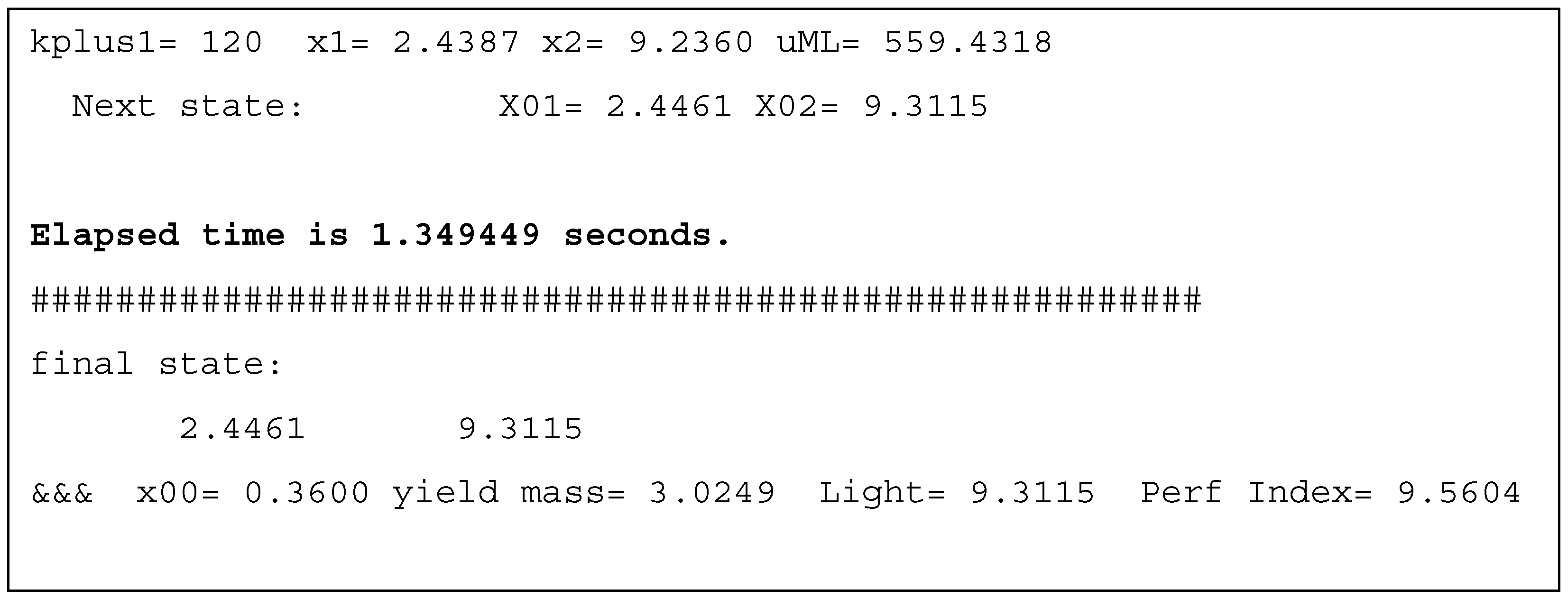
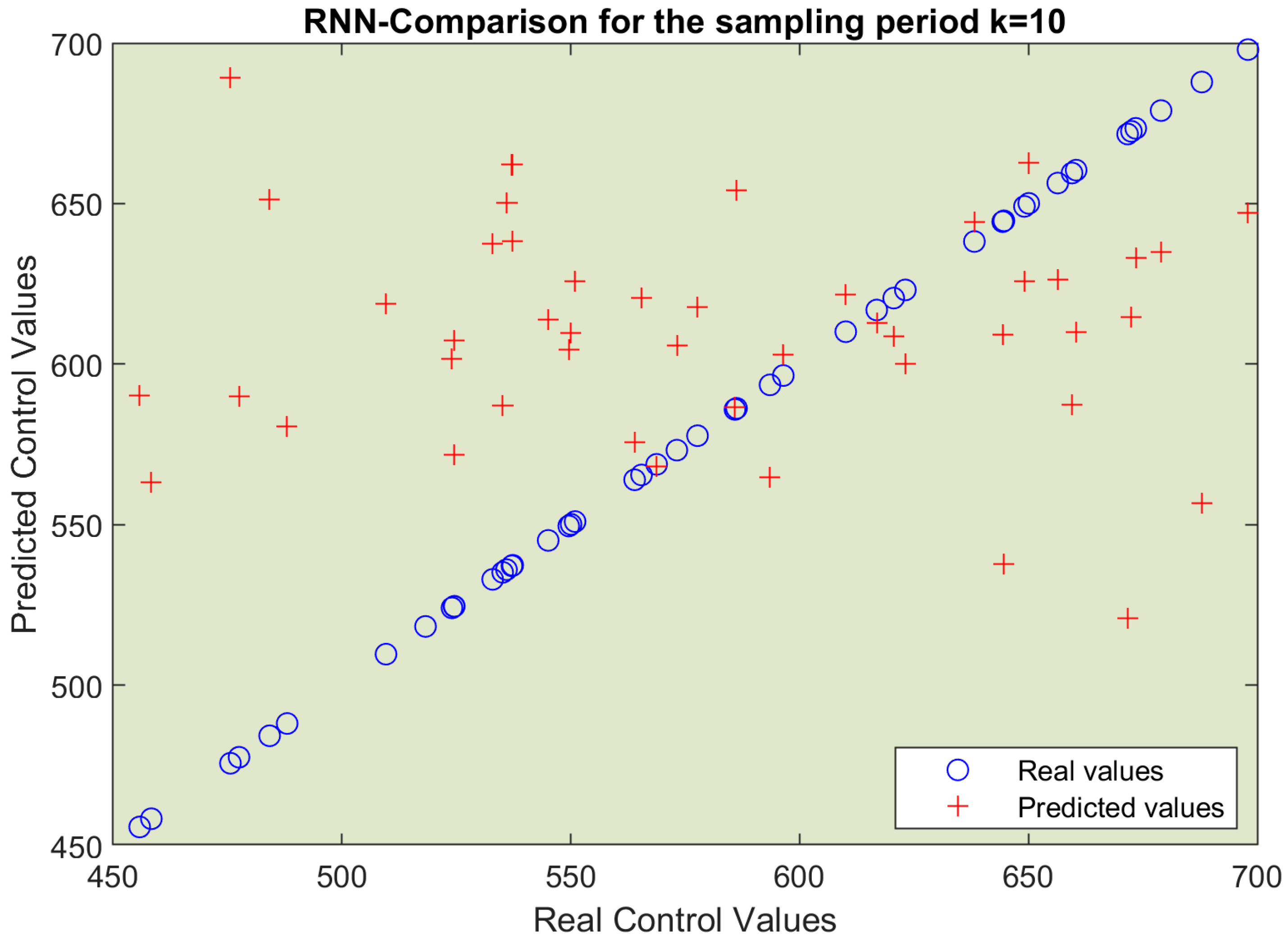
6.2. Simulation Results
7. Discussion
7.1. Comparison between PSO and ML Predictors
- Did the ML predictors succeed in “learning” the behavior of the couple (APSOA and PM), such that the process’s evolution would be quasi-optimal?
- Did the controller’s execution time decrease significantly?
- The similarity at this level would imply the same sequences of states, but we just stated that the ML controllers could experience new unobserved states. So, the three processes do not pass through the same set of states (the sets of accessible states are different).
- The learning is made at the level of each sampling period and the model “learns” couples (state; control value), not globally, but at the control profile level; our method is not based on learning CPs. On the other hand, the PSO predictor is very “noisy” due to its stochastic character and produces outliers among the 200 control values from time to time.
- The two ML controllers have predictors that have learned the behavior of the couple (APSOA and PM), such that in closed-loop functioning, the process evolves almost identically.
- The resulting controllers have execution times hundreds of times smaller than that of the PSO Controller.
7.2. Comparison between the LR and RNN Controllers
- The ML predictor replaces the PSO predictor only in execution when the controller achieves the control action. So, the controller’s execution time is hundreds of times smaller compared to initially. That was our desideratum.
- When we solve a new OCP, sometimes we need a metaheuristic (PSO, EA, etc.) that searches for the optimal solution inside of a control structure. If the controller’s execution time is not acceptable, we can use the approach presented in this paper to create an ML controller. However, initially, we need the MA to search for the optimal solution.
8. Conclusions
- The machine learning models succeed in “learning” the quasi-optimal behavior of the couple (PSO and PM) using data capturing the PSO predictor’s behavior. The training data are the optimal control profiles and trajectories recorded during M offline simulations of the closed-loop over the control horizon.
- The current paper proposes algorithms for collecting data and aggregating data sets for the learning process. The learning process is split according to the level of each sampling period so that a predictor model is trained for each one. The multiple linear regression and the Regression Neural Networks are considered the predicting models.
- For each case, we propose algorithms for constructing the set of ML models and the controller (LR or RNN controller). Algorithms for the closed-loop simulations using the two controllers are also proposed; they allow us to compare the process evolutions involved by the three controllers, the PSO, LR, and RNN controllers.
- The final simulations show that the new controllers preserve the quasi-optimality of the process evolution. In the same conditions, the process evolutions are almost identical.
- An advantage of our approach refers to data collection, data set preparation for the training process, and the construction of ML models; all of these activities need only simulations (using the PSO controller) and offline program executions (Remark 6). The ML models for each sampling period are determined offline ahead of using the ML controller in real time.
- We emphasize that during the final closed-loop simulations, the ML controller encounters new process states unobserved in the training and testing of its predictor (Remark 10). Owing to its generalization ability, the controller makes accurate predictions of the control value sent to the process.
Supplementary Materials
Author Contributions
Funding
Data Availability Statement
Acknowledgments
Conflicts of Interest
Appendix A

| = 172 m2·kg−1 | absorption coefficient |
| = 870 m2·kg−1 | scattering coefficient |
| = 0.0008 | backward scattering fraction |
| = 0.16 h−1 | specific growth rate |
| = 0.013 h−1 | specific decay rate |
| = 120 µmol·m−2·s−1 | saturation constant |
| = 2500 µmol·m−2·s−1 | inhibition constant |
| = 1.45·10−3 m3 | volume of PBR |
| L = 0.04 m | depth of PBR |
| A = 3.75·10−2 m2 | lighted surface |
| = 0.36 g/L | initial biomass concentration |
| C =3600·10−2 | light-intensity conversion constant |
| = 100 | number of discretization points |
| lower technological light intensity | |
| upper technological light intensity | |
| = 3 g. | minimal final biomass |
| tfinal = 120 h | control horizon |
| T = 1 h | sampling period |
Appendix B
- ControlLoop_PSO_RHC.m that implements the “ControlLoop_PSO” program;
- INV_PSO_Predictor1.m that implements the “Predictor_PSO” function;
- INV_RealProcessStep.m that implements the “ProcessStep” function.

Appendix C
| x1 | x2 | u | |
|---|---|---|---|
| i = 1 | 0.37831 | 0.094853 | 612.65 |
| i = 2 | 0.40708 | 0.077925 | 557.37 |
| i = 3 | 0.40122 | 0.066811 | 802.69 |
| i = 4 | 0.40359 | 0.079127 | 387.99 |
| i = 5 | 0.37865 | 0.078882 | 560.77 |
| i = 6 | 0.37801 | 0.079205 | 510.57 |
| … | … | … | … |
| … | … | … | … |
| i = 197 | 0.40607 | 0.074351 | 547.26 |
| i = 198 | 0.39419 | 0.069684 | 485.64 |
| i = 199 | 0.38625 | 0.082921 | 558.9 |
| i = 200 | 0.39531 | 0.071325 | 539.92 |
Appendix D
The Linear Regression Models’ Construction


Appendix E
‘LayerSizes’, [14 1 7], …
‘Activations’, ‘none’, …
‘Lambda’, 0.00015, …
‘IterationLimit’, 1000, …
‘Standardize’, true);

References
- Siarry, P. Metaheuristics; Springer: Berlin/Heidelberg, Germany, 2016; ISBN 978-3-319-45403-0. [Google Scholar]
- Talbi, E.G. Metaheuristics—From Design to Implementation; Wiley: Hoboken, NJ, USA, 2009; ISBN 978-0-470-27858-1. [Google Scholar]
- Kruse, R.; Borgelt, C.; Braune, C.; Mostaghim, S.; Steinbrecher, M. Computational Intelligence—A Methodological Introduction, 2nd ed.; Springer: Berlin/Heidelberg, Germany, 2016. [Google Scholar]
- Tian, G.; Zhang, L.; Fathollahi-Fard, A.M.; Kang, Q.; Li, Z.; Wong, K.Y. Addressing a Collaborative Maintenance Planning Using Multiple Operators by a Multi-Objective Metaheuristic Algorithm. IEEE Trans. Autom. Sci. Eng. 2023, 7, 1–13. [Google Scholar] [CrossRef]
- Onwubolu, G.; Babu, B.V. New Optimization Techniques in Engineering; Springer: Berlin/Heidelberg, Germany, 2004. [Google Scholar]
- Valadi, J.; Siarry, P. Applications of Metaheuristics in Process Engineering; Springer International Publishing: Berlin/Heidelberg, Germany, 2014; pp. 1–39. [Google Scholar] [CrossRef]
- Abraham, A.; Jain, L.; Goldberg, R. Evolutionary Multi-objective Optimization—Theoretical Advances and Applications; Springer: Berlin/Heidelberg, Germany, 2005; ISBN 1-85233-787-7. [Google Scholar]
- Minzu, V.; Serbencu, A. Systematic procedure for optimal controller implementation using metaheuristic algorithms. Intell. Autom. Soft Comput. 2020, 26, 663–677. [Google Scholar] [CrossRef]
- Hu, X.B.; Chen, W.H. Genetic algorithm based on receding horizon control for arrival sequencing and scheduling. Eng. Appl. Artif. Intell. 2005, 18, 633–642. [Google Scholar] [CrossRef]
- Mayne, D.Q.; Michalska, H. Receding Horizon Control of Nonlinear Systems. IEEE Trans. Autom. Control 1990, 35, 814–824. [Google Scholar] [CrossRef]
- Mînzu, V.; Rusu, E.; Arama, I. Execution Time Decrease for Controllers Based on Adaptive Particle Swarm Optimization. Inventions 2023, 8, 9. [Google Scholar] [CrossRef]
- Goggos, V.; King, R. Evolutionary predictive control. Comput. Chem. Eng. 1996, 20 (Suppl. S2), S817–S822. [Google Scholar] [CrossRef]
- Chiang, P.-K.; Willems, P. Combine Evolutionary Optimization with Model Predictive Control in Real-time Flood Control of a River System. Water Resour. Manag. 2015, 29, 2527–2542. [Google Scholar] [CrossRef]
- Wu, J.; Zhang, C.; Giam, A.; Chia, H.Y.; Cao, H.; Ge, W.; Yan, W. Physics-assisted transfer learning metamodels to predict bead geometry and carbon emission in laser butt welding. Appl. Energy 2024, 359, 122682. [Google Scholar] [CrossRef]
- Minzu, V.; Riahi, S.; Rusu, E. Implementation aspects regarding closed-loop control systems using evolutionary algorithms. Inventions 2021, 6, 53. [Google Scholar] [CrossRef]
- Minzu, V.; Georgescu, L.; Rusu, E. Predictions Based on Evolutionary Algorithms Using Predefined Control Profiles. Electronics 2022, 11, 1682. [Google Scholar] [CrossRef]
- Banga, J.R.; Balsa-Canto, E.; Moles, C.G.; Alonso, A. Dynamic optimization of bioprocesses: Efficient and robust numerical strategies. J. Biotechnol. 2005, 117, 407–419. [Google Scholar] [CrossRef] [PubMed]
- Balsa-Canto, E.; Banga, J.R.; Aloso, A.V. Vassiliadis. Dynamic optimization of chemical and biochemical processes using restricted second-order information 2001. Comput. Chem. Eng. 2001, 25, 539–546. [Google Scholar] [CrossRef]
- Mînzu, V.; Arama, I. A Machine Learning Algorithm That Experiences the Evolutionary Algorithm’s Predictions—An Application to Optimal Control. Mathematics 2024, 12, 187. [Google Scholar] [CrossRef]
- Minzu, V.; Riahi, S.; Rusu, E. Optimal control of an ultraviolet water disinfection system. Appl. Sci. 2021, 11, 2638. [Google Scholar] [CrossRef]
- Minzu, V.; Ifrim, G.; Arama, I. Control of Microalgae Growth in Artificially Lighted Photobioreactors Using Metaheuristic-Based Predictions. Sensors 2021, 21, 8065. [Google Scholar] [CrossRef] [PubMed]
- Goodfellow, I.; Bengio, Y.; Courville, A. Machine Learning Basics. In Deep Learning; The MIT Press: Cambridge, MA, USA, 2016; pp. 95–161. ISBN 978-0262035613. [Google Scholar]
- Zou, S.; Chu, C.; Shen, N.; Ren, J. Healthcare Cost Prediction Based on Hybrid Machine Learning Algorithms. Mathematics 2023, 11, 4778. [Google Scholar] [CrossRef]
- Cuadrado, D.; Valls, A.; Riaño, D. Predicting Intensive Care Unit Patients’ Discharge Date with a Hybrid Machine Learning Model That Combines Length of Stay and Days to Discharge. Mathematics 2023, 11, 4773. [Google Scholar] [CrossRef]
- Albahli, S.; Irtaza, A.; Nazir, T.; Mehmood, A.; Alkhalifah, A.; Albattah, W. A Machine Learning Method for Prediction of Stock Market Using Real-Time Twitter Data. Electronics 2022, 11, 3414. [Google Scholar] [CrossRef]
- Wilson, C.; Marchetti, F.; Di Carlo, M.; Riccardi, A.; Minisci, E. Classifying Intelligence in Machines: A Taxonomy of Intelligent Control. Robotics 2020, 9, 64. [Google Scholar] [CrossRef]
- Alatefi, S.; Abdel Azim, R.; Alkouh, A.; Hamada, G. Integration of Multiple Bayesian Optimized Machine Learning Techniques and Conventional Well Logs for Accurate Prediction of Porosity in Carbonate Reservoirs. Processes 2023, 11, 1339. [Google Scholar] [CrossRef]
- Guo, R.; Zhao, Z.; Huo, S.; Jin, Z.; Zhao, J.; Gao, D. Research on State Recognition and Failure Prediction of Axial Piston Pump Based on Performance Degradation Data. Processes 2020, 8, 609. [Google Scholar] [CrossRef]
- Newbold, P.; Carlson, W.L.; Thorne, B. Multiple Regression. In Statistics for Business and Economics, 6th ed.; Pfaltzgraff, M., Bradley, A., Eds.; Pearson Education, Inc.: Upper Saddle River, NJ, USA, 2007; pp. 454–537. [Google Scholar]
- The MathWorks Inc. Stepwise Regression Toolbox Documentation; The MathWorks Inc.: Natick, MA, USA, 2024; Available online: https://www.mathworks.com/help/stats/stepwise-regression.html (accessed on 2 September 2023).
- Goodfellow, I.; Bengio, Y.; Courville, A. Example: Linear Regression. In Deep Learning; The MIT Press: Cambridge, MA, USA, 2016; pp. 104–113. ISBN 978-0262035613. [Google Scholar]
- The MathWorks Inc. Regression Neural Network Toolbox Documentation; The MathWorks Inc.: Natick, MA, USA, 2024; Available online: https://www.mathworks.com/help/stats/regressionneuralnetwork.html (accessed on 2 September 2023).


| XT | UT |
|---|---|
| …… | …… |
| /*This pseudocode describes the construction of the data sets needed by the ML models at the level of each sampling period*/ Inputs: cell array STATE, matrix UstarRHC; Outputs: matrix SOCSK, table datak, cell arrays DATAKTest, DATAKTrain | |
| 1. | #Load the file containing the data structure STATE and UstarRHC (Figure A1) |
| 2. | |
| 3. | while |
| 4. | for i = 1, ∙∙∙, M |
| 5. | |
| 6. | end |
| 7. | #Convert the matrix SOCSK into the table datak. |
| 8. | datakTest ← lines #1—60 of datak |
| 9. | datakTrain ← lines #61—120 of datak |
| 10. | DATAKTest{k} ← datakTest |
| 11. | DATAKTrain{k} ← datakTrain |
| 12. | |
| 13. | end |
| 14. | #Save the cell array DATAKTrain and DATAKTest in a file. |
| The General Algorithm of the ML Controller | |
|---|---|
| /*The controller program is called at each sampling period, k */ | |
| 1 | Get the current value of the state vector, X(k); /* Initialize */ |
| 2 | Predict the optimal control value using the regression model /* whatever is the regression model’s type */ |
| 3 | Send the optimal control value towards the process. |
| 4 | Wait for the next sampling period. |
| Construction of the linear regression models Input: cell arrays DATAKTrain, DATAKTest Output: matrix KOEF (), /* the regression coefficients for each sampling period */ cell array MODELSW {} /* cell array storing objects that are the linear models */ | |
| 1 | for k = 0…H-1. |
| 2 | datakTrain DATAKTrain{k}; /* Recover the data set for training */ |
| 3 | datakTest DATAKTest{k}; /* Recover the data set for testing */ |
| 4 | mdlswfitting_to_data(datakTrain); /* Training the linear regression */ |
| 5 | #display mdlsw; /* mdlsw is the linear regression model */ |
| 6 | coef(:)get_the_coefficients(mdl) |
| 7 | KOEF(k,:) coef(:); /* The kth line of KOEF receives the coefficients */ |
| 8 | MODELSWP{k,1}mdlsw; |
| 9 | uPred fpredict(mdlsw, datakTest) /* The vector uPred stores the predicted control values */ |
| 10 | # Make the comparison between uPred and the real control values; |
| 11 | end. |
| &&&&kp1 = 14 | ||||
| 1. Adding x1, FStat = 12.7755, p Value = 0.000484491 | ||||
| Linear regression model: u ~ 1 + x1 | ||||
| Estimated Coefficients: | ||||
| Estimate | SE | tStat | p Value | |
| (Intercept) | −985.91 | 437.95 | −2.2512 | 0.025952 |
| x1 | 2147.7 | 600.87 | 3.5743 | 0.00048449 |
| Number of observations: 140; Error degrees of freedom: 138 Root mean square error: 117 R-squared: 0.0847; Adjusted R-squared: 0.0781 F-statistic vs. constant model: 12.8; p-value = 0.000484 | ||||
| k | C0 | C1 | C2 |
|---|---|---|---|
| 0 | 564.18 | 0 | |
| 1 | 585.53 | 0 | 0 |
| 2 | −20.368 | 1441.5 | 0 |
| : | : | : | : |
| 9 | 591.85 | 0 | 0 |
| 10 | 119.74 | 0 | 620.84 |
| 11 | 591.48 | 0 | 0 |
| 12 | 590.95 | 0 | 0 |
| 13 | −985.91 | 2147.7 | 0 |
| 14 | −328.16 | 1205.6 | 0 |
| : | : | : | : |
| 111 | 4055.1 | −1476.6 | 0 |
| 112 | 5482.6 | −2067.6 | 0 |
| 113 | 597.8 | 0 | 0 |
| 114 | 3300.2 | 0 | −308.67 |
| 115 | 587.66 | 0 | 0 |
| 116 | 6446.3 | −2451.2 | 0 |
| 117 | 7144 | −2732.8 | 0 |
| 118 | 4410.7 | 0 | −419.32 |
| 119 | 565.2 | 0 | 0 |
| Construction of the RNN models Input: cell arrays DATAKTrain, DATAKTest Output: cell array MODELNN {} /* cell array storing objects that are RNN */ | |
| 1 | for k = 0…H-1. |
| 2 | datakTrain DATAKTrain{k, 1}; /* Recover the data set for training */ |
| 3 | datakTest DATAKTest{k, 1}; /* Recover the data set for testing */ |
| 4 | mdlNNtrainRegNN(datakTrain); /* Training the RNN */ |
| 5 | MODELNN{k,1}mdlNN /* Store the object mdlNN into the cell array MODELNN */ |
| 6 | predictionNNmdlNN.predictFcn(datakTest) /* Make predictions and store them into the table predictionNN */ |
| 7 | # Comparison between predictionNN and datakTest |
| 8 | end |
| >> GENERATE_ModelNN |
| &&& vrmse = 108.4187 RMSEValid = 111.9601 kplus1 = 1 uNN = 564.1789 valreal = 487.0276 &&& vrmse = 104.5341 RMSEValid = 130.6362 kplus1 = 2 uNN = 574.4657 valreal = 672.5530 &&& vrmse = 106.0061 RMSEValid = 127.3596 kplus1 = 3 uNN = 559.1601 valreal = 676.6160 ---------------------- &&& vrmse = 112.0696 RMSEValid = 91.4825 kplus1 = 119 uNN = 588.0487 valreal = 634.9497 &&& vrmse=130.1694 RMSEValid = 125.2698 kplus1 = 120 uNN = 576.2782 valreal = 714.3906 Elapsed time is 232.829571 s. |
| >>ControlLoop_PSO_RHC |
| x00 = 0.3660 |
| Yield mass = 3.0000 |
| Light = 9.2474 |
| Perf index = 9.2474 |
| Elapsed time is 447.281879 s. |
| PSO Controller | LR Controller | RNN Controller | |
|---|---|---|---|
| x00 | 0.360 | 0.360 | 0.360 |
| Yield mass | 3.0000 | 3.0282 | 3.0249 |
| Light | 9.2474 | 9.3166 | 9.3115 |
| Perf index | 9.2474 | 9.5981 | 9.5604 |
| Control time [s] | 447.28 | 0.64 | 1.35 |
| Training time [s] | - | 5.4 | 232.83 |
| Model size | - | 3 kB | 17 kB |
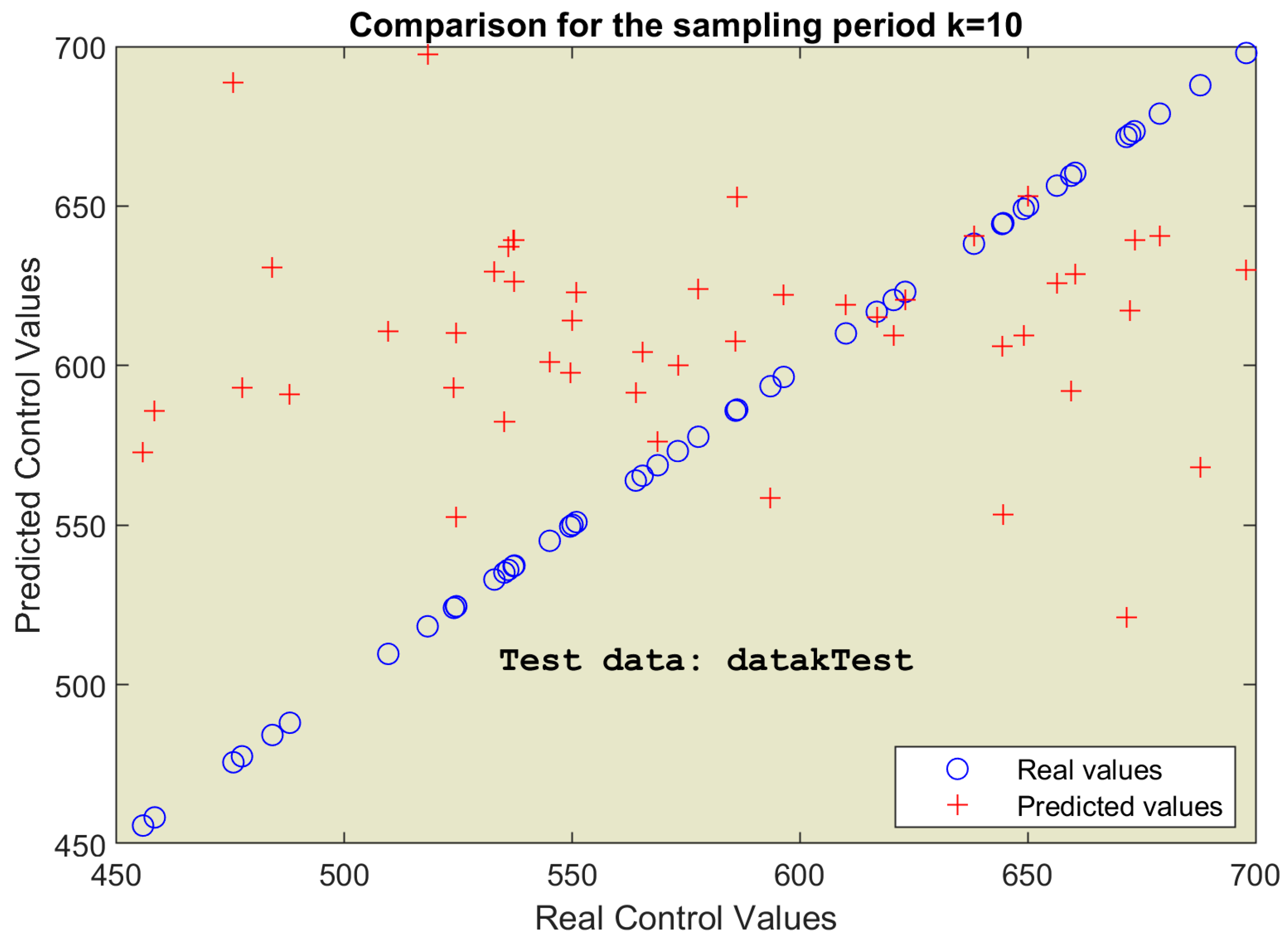
| Root mean square error (RMSE for k = 10) | - | 113.73 | 116.63 |
Disclaimer/Publisher’s Note: The statements, opinions and data contained in all publications are solely those of the individual author(s) and contributor(s) and not of MDPI and/or the editor(s). MDPI and/or the editor(s) disclaim responsibility for any injury to people or property resulting from any ideas, methods, instructions or products referred to in the content. |
© 2024 by the authors. Licensee MDPI, Basel, Switzerland. This article is an open access article distributed under the terms and conditions of the Creative Commons Attribution (CC BY) license (https://creativecommons.org/licenses/by/4.0/).
Share and Cite
Mînzu, V.; Arama, I.; Rusu, E. Machine Learning Algorithms That Emulate Controllers Based on Particle Swarm Optimization—An Application to a Photobioreactor for Algal Growth. Processes 2024, 12, 991. https://doi.org/10.3390/pr12050991
Mînzu V, Arama I, Rusu E. Machine Learning Algorithms That Emulate Controllers Based on Particle Swarm Optimization—An Application to a Photobioreactor for Algal Growth. Processes. 2024; 12(5):991. https://doi.org/10.3390/pr12050991
Chicago/Turabian StyleMînzu, Viorel, Iulian Arama, and Eugen Rusu. 2024. "Machine Learning Algorithms That Emulate Controllers Based on Particle Swarm Optimization—An Application to a Photobioreactor for Algal Growth" Processes 12, no. 5: 991. https://doi.org/10.3390/pr12050991
APA StyleMînzu, V., Arama, I., & Rusu, E. (2024). Machine Learning Algorithms That Emulate Controllers Based on Particle Swarm Optimization—An Application to a Photobioreactor for Algal Growth. Processes, 12(5), 991. https://doi.org/10.3390/pr12050991