Local Path Planner for Mobile Robot Considering Future Positions of Obstacles

Abstract

Local path planning is a necessary ability for mobile robot navigation, but existing planners are not sufficiently effective at dynamic obstacle avoidance. In this article, an improved timed elastic band (TEB) planner based on the requirements of mobile robot navigation in dynamic environments is proposed. The dynamic obstacle velocities and TEB poses are fully integrated through two-dimensional (2D) lidar and multi-obstacle tracking. First, background point filtering and clustering are performed on the lidar points to obtain obstacle clusters. Then, we calculate the data association matrix of the obstacle clusters of the current and previous frame so that the clusters can be matched. Thirdly, a Kalman filter is adopted to track clusters and obtain the optimal estimates of their velocities. Finally, the TEB poses and obstacle velocities are associated: we predict the obstacle position corresponding to the TEB pose through the detected obstacle velocity and add this constraint to the corresponding TEB pose vertex. Then, a pose sequence considering the future positions of obstacles is obtained through a graph optimization algorithm. Compared with the original TEB, our method reduces the total running time by 22.87%, reduces the running distance by 19.23%, and increases the success rate by 21.05%. Simulations and experiments indicate that the improved TEB enables robots to efficiently avoid dynamic obstacles and reach the goal as quickly as possible.

1. Introduction

Wheeled mobile robots are increasingly used in today’s society in such forms as food delivery robots and transportation robots. In the autonomous navigation of robots, avoiding obstacles and safely reaching the target are the challenges they encounter, especially in the face of dynamic obstacles, and the robot must process a large amount of environmental information and make optimal control decisions. After the robot receives the reference path given by the global path planner [1,2], the local path planner needs to give the robot an optimal local path through sensors such as cameras, lidar, or ultrasonic devices so that the mobile robot can reach the target as soon as possible while avoiding obstacles on the path.

Obstacle detection plays a key role in the navigation of mobile robots in dynamic environments. This is the main way for mobile robots to receive obstacle motion information. Many recent object detection algorithms are vision-based [3,4]; these need a large amount of calculations, and vision-based object detection is greatly affected by light. Of course, some people use low-cost sensors such as infrared sensors for detecting obstacles [5]. Although the amount of calculation is small, there is too little information, so in this article, we weigh the pros and cons of using two-dimensional lidar to detect obstacle movement information [6,7,8,9,10,11]. We think that for robots, the data provided by 2D lidar can basically meet the robot’s obstacle avoidance needs because for robot obstacle avoidance, we only need to consider obstacle detection rather than obstacle recognition.

Local planners include the dynamic window approach (DWA) and TEB. The DWA [12] mainly samples multiple groups of velocities in the linear and angular velocity space, simulates the trajectories formed by these velocities within a certain time period, evaluates these trajectories through the evaluation function, and selects the best trajectory. Its advantage is low computational complexity and strong real-time performance. The disadvantage is that it easily becomes stuck in local optimal, and it is suitable only for certain robots. The TEB [13,14,15,16] local planner’s working principle is to insert N time intervals of T seconds between the start and target. Then, it finds the optimal pose sequence through the optimization algorithm and motion instructions to drive the robot to the target. In the Robot Operating System (ROS), TEB is an open-source package. The optimization method uses the general graph optimization (G2O) algorithm [17].

The two classic algorithms mentioned above can basically realize the local planning for most robots in most static environments, but these algorithms do not take the movement information of obstacles into consideration, and they all regard obstacles as static obstacles, which causes the planned trajectory to be only currently optimal, regardless of the future positions of the obstacles, so the obstacle avoidance effect in a dynamic environment is not good enough. However, robot obstacle avoidance is systematic work that not only needs path planners [18,19] but also needs to combine obstacle perception [20,21], robot control [22], trajectory tracking [23,24], and localization [25,26,27].

Therefore, on the basis of the TEB algorithm structure, we use 2D lidar to fully integrate dynamic obstacle velocities and finally plan a collision-free trajectory considering the future positions of obstacles. First, the robot receives a 2D point set through lidar and obtains obstacle point clusters through operations such as coordinate transformation, background point filtering, and obstacle point clustering. Then, a Kalman filter [28] is used to track obstacles to obtain obstacle velocities. Afterward, the velocities of obstacles are used to predict the future positions of the obstacles for various TEB poses; then, the robot optimizes the trajectory by the G2O method to obtain a collision-free trajectory.

The main contributions of this manuscript are as follows:

• A multi-obstacle velocities detection algorithm through 2D lidar and Kalman filter is proposed.
• An improved TEB local planner that combines the TEB poses and obstacle velocities is designed to improve the robot’s dynamic obstacle avoidance efficiency.
• A series of simulations and experiments are performed to verify the effectiveness of the proposed method.

2. Related Work

Path planning in response to dynamic obstacles is an open research topic that has been studied for decades. There are many obstacle avoidance algorithms for dynamic environments, but many of these algorithms were initially proposed for static environments and then adapted to dynamic environments, including artificial potential field (APF), DWA, and TEB. The APF [29] algorithm is a typical reactive method. It uses repulsion and attraction to plan the local trajectory of the robot. Attraction is positively correlated with the distance between the robot and the target, while repulsion is the opposite. This algorithm has a simple structure, but there are many defects. For example, it does not consider the kinematics of the robot, and it can easily fall into a local optimum; moreover, the algorithm does not take the future positions of obstacles into consideration. Methods based on velocity obstacle (VO) [30,31,32,33] are also noteworthy reactive methods that utilize the collision region principle to detect regions where collisions are possible for dynamic obstacle avoidance. Although these reactive methods are effective at obstacle avoidance, there is still considerable room for improvement. The application of the original TEB algorithm in dynamic scenes only continuously updates the local cost map without considering the statuses of obstacles. In this situation, if the speed of the robot or obstacle is too fast, the robot may not be able to successfully avoid obstacles.

There are some recent studies considering dynamic obstacles. Guo [34] proposed an obstacle avoidance algorithm suitable for two-wheeled differential-driven robots by using a stereo vision system to detect dynamic obstacles, estimating the motion state of dynamic obstacles through an extended Kalman filter, and then by using the velocities of obstacles to calculate dynamic risk regions and realize dynamic obstacle avoidance for the robot. However, it can be applied to only the differential speed robot. For pedestrians, a special type of obstacle avoidance model has been proposed: Reddy [35] is a hybrid path planning method that takes into account some navigation habits of pedestrians walking, such as avoiding obstacles from the left side. Using these behaviors as a reference, the method combines the social force field with geometric methods to select the optimal path for the robot. According to experimental results, this algorithm outperforms baseline and individual methods. Smith [36] combines path planning with reinforcement learning and proposes a cooperative Markov decision process (Co-MDP) approach. This method utilizes an MDP to predict human behavior and integrates the prediction results with social rules and the state of the robot; the research aims to humanize the robot’s movements, and the robot performs well in human–robot co-populated environments. Chen and Lin [37] provided a plugin of the cost map2d [38] layer in the framework of the ROS. On the basis of the obstacle layer and the obstacle expansion layer, the obstacle velocity layer was introduced. This layer passed the DeepSort [39] algorithm to detect dynamic obstacles, to further extract 2D lidar messages, and to generate moving obstacles and the range of future moments through the k-means clustering algorithm; this method provides better trajectory planning for mobile robots to avoid obstacles in dynamic environments. Dong [40] proposed an algorithm that combines two-dimensional lidar and the TEB algorithm. Simulation and experiments have proven the ability of the system in real-time detection and obstacle tracking and show that it has a certain robustness. Wang [41] set up a virtual target (VT) on the global path and tracked the VT and tracked the global path when the robot was moving in the dynamic environment to achieve safe and stable operation of the robot in a dynamic environment. In this article, we also propose a global path replanning strategy to address the situation of untrackable areas in dense environments. Through a large number of experiments, it is proven that this method can reach the target faster, safer, and more smoothly than can other methods.

3. Methodology

In this section, we first introduce how to use 2D lidar for obstacle detection, and then, we describe the details of obstacle tracking when using the Kalman filter and the calculation of the interframe data association matrix. Finally, we introduce how to use obstacle velocities and TEB pose information to predict the obstacle positions of different poses in the future as well as a method for associating TEB pose vertices and obstacle edges.

3.1. Obstacle Detection

3.1.1. Clustering

A point set obtained by 2D lidar is based on the polar coordinate system with the lidar as the origin and consists of the polar diameter and polar angle; the expression is $(\theta ,r)$. However, this form of data does not satisfy our requirements for obstacle velocity detection, so we need to transform it into the coordinate system $(x,y)$ with the map as the origin. Therefore, this algorithm relies more on the accuracy of the real-time localization algorithm of the robot. The formula to transform the coordinates from $(\theta ,r)$ to $(x,y)$ is as follows:

$$\left[\begin{array}{c}x\\ y\end{array}\right]=\left[\begin{array}{cc}cos{\theta }_r& -sin{\theta }_r\\ sin{\theta }_r& cos{\theta }_r\end{array}\right]\times \left[\begin{array}{c}cos\theta \\ sin\theta \end{array}\right]\times r+\left[\begin{array}{c}{x}_r\\ y_r\end{array}\right]$$

(1)

where $(x_r,y_r,{\theta }_r)$ is the robot’s global pose in the map, $(x_r,y_r)$ are the coordinates and ${\theta }_r$ is the orientation of the robot, $(x,y)$ are the point coordinates after transformation, while $(\theta ,r)$ are the polar coordinate points before.

After obtaining the global point cloud, these points need to be clustered. This paper uses the conditional Euclidean clustering algorithm to cluster the point set and uses the known inflated global grid map as a mask to filter out the background points; this clustering results in K obstacle clusters. Figure 1 presents the schematic diagram of background point clustering. The original Euclidean has only one hyperparameter: that is, $ϵ$, which is the neighborhood range. The setting of this hyperparameter will depend on the width of the mobile robot, the pedestrian’s step length, and the resolution of the lidar. Conditional Euclidean clustering adds a hyperparameter based on the original algorithm: that, is the background grid map after inflation. Whenever the clustering algorithm searches for a point, in addition to judging how the point cloud is distanced from the neighboring points, the background map will also be used to determine whether the point is a noise point. After the points are clustered, K clusters will be obtained. In addition, the length and width of each cluster needs to be calculated to facilitate the subsequent calculation of the intersection over union (IOU).

3.1.2. Data Association Matrix

Calculation of the data association matrix is crucial in multi-obstacle tracking because it is necessary to ensure that the clusters of the current frame corresponds to the clusters of the previous frame. The calculation method of the data association matrix in this article is introduced below. First, the expression of the obstacle cluster center set obtained by clustering is as follows:

$$P^{pre}\triangleq \{(p{x}_i^{pre},p{y}_i^{pre}),i\in [1,M]\}$$

(2)

$$P^{now}\triangleq \{(p{x}_j^{now},p{y}_j^{now}),j\in [1,K]\}$$

(3)

where $P^{pre}$ is the cluster set in the previous frame, $P^{now}$ is the cluster set in the current frame, and M and K are the total number of point cloud cluster sets. Then, the data association matrix $mat$ is weighted by two matrices: a distance difference matrix $ma{t}_{dist}$ and an IOU matrix $ma{t}_{IOU}$. The specific expansion formula is as follows:

$$mat=\alpha \times ma{t}_{dist}+\beta \times ma{t}_{IOU}$$

(4)

$$ma{t}_{dist}=\left[\begin{array}{ccc}d{(p_1^{pre},p_1^{now})}^{-1}& \cdots & d{(p_1^{pre},p_K^{now})}^{-1}\\ ⋮& \ddots & ⋮\\ d{(p_M^{pre},p_1^{now})}^{-1}& \cdots & d{(p_M^{pre},p_K^{now})}^{-1}\end{array}\right]$$

(5)

$$ma{t}_{IOU}=\left[\begin{array}{ccc}IOU(p_1^{pre},p_1^{now})& \cdots & IOU(p_1^{pre},p_K^{now})\\ ⋮& \ddots & ⋮\\ IOU(p_M^{pre},p_1^{now})& \cdots & IOU(p_M^{pre},p_K^{now})\end{array}\right]$$

(6)

The expansion of the data in the matrix $ma{t}_{dist}$ is as follows (that is, the distance between the center of the i-th cluster in the previous frame and the j-th cluster in the current frame):

$$d(p_i^{pre},p_j^{now})=\sqrt{{(x_i^{pre}-x_j^{now})}^2+{(y_i^{pre}-y_j^{now})}^2}$$

(7)

The specific meaning of the data in the matrix $ma{t}_{IOU}$ is the intersection and union ratio between the current cluster and the previous frame. The IOU is the intersection ratio and the union of the binding boxes of the two clusters. Finally, we get a value between (0, 1).

In addition, in order to eliminate the dimensional influence between different features and to improve the matching accuracy, the two matrices need to be normalized: the original data are linearly mapped to the [0, 1] interval, and the mapping function is:

$$x^{\prime }=(x-min)/(max-min)$$

(8)

where x are the original data, $x^{\prime }$ are the normalized data, $min$ is the minimum value in the matrix, and $max$ is the maximum value in the matrix.

3.1.3. Kalman Filter Tracking

The pairing relationship of clusters between frames can be obtained through the data association matrix, and then, the obstacles are tracked through Kalman filtering to obtain their motion information. The state equation of the obstacles is:

$$X_t=A{X}_{t-1}+W_{t-1}$$

(9)

where $X_t={[x,y,v^x,v^y,a^x,a^y]}^T$ is a six-dimensional state vector that includes position, velocity, and acceleration in the x- and y-directions. $X_{t-1}$ is the state at the previous moment, and $W_{t-1}$ is the process noise, for which the probability distribution is unknown. A is the state transition matrix; the expansion of this matrix is as follows:

$$A=\left[\begin{array}{cccccc}1& 0& dt& 0& d{t}^2/2& 0\\ 0& 1& 0& dt& 0& d{t}^2/2\\ 0& 0& 1& 0& dt& d{t}^2/2\\ 0& 0& 0& 1& 0& dt\\ 0& 0& 0& 0& 1& 0\\ 0& 0& 0& 0& 0& 1\end{array}\right]$$

(10)

where $dt$ is the observation interval: that is, the time interval between frames. The observation matrix for dynamic obstacles is:

$$Z_t=H{X}_t+V_t$$

(11)

where $Z_t={[x,y,v^x,v^y]}^T$ is the observation value and includes the coordinates and velocities of the obstacle in the x- and y-directions. Observations come from inter-frame clusters: from such clusters we obtain the positions of the obstacles. Referring to the idea of differentiation, $v^x$ and $v^y$ can be obtained. As long as the sampling interval $dt$ is small enough, the obstacles in the two sampling intervals can be seen to move at a uniform speed: that is $v_t^x=(x_t-x_{t-1})/dt$. Similarly, $v_t^y$, $V_t$ is observation noise. The observation matrix H is:

$$H=\left[\begin{array}{cccc}1& 0& 0& 0\\ 0& 1& 0& 0\\ 0& 0& 1& 0\\ 0& 0& 0& 1\end{array}\right]$$

(12)

The posterior estimate ${\widehat{X}}_t$ is calculated through the Kalman gain from the following equation:

$${\widehat{X}}_t={\widehat{X}}_t^{-}+K_t(Z_t-H{\widehat{X}}_t^{-})$$

(13)

The term ${\widehat{X}}_t$ is the optimal motion estimates of obstacles. Following, we introduce how to associate motion information with the original TEB algorithm to achieve local planning and dynamic obstacle avoidance.

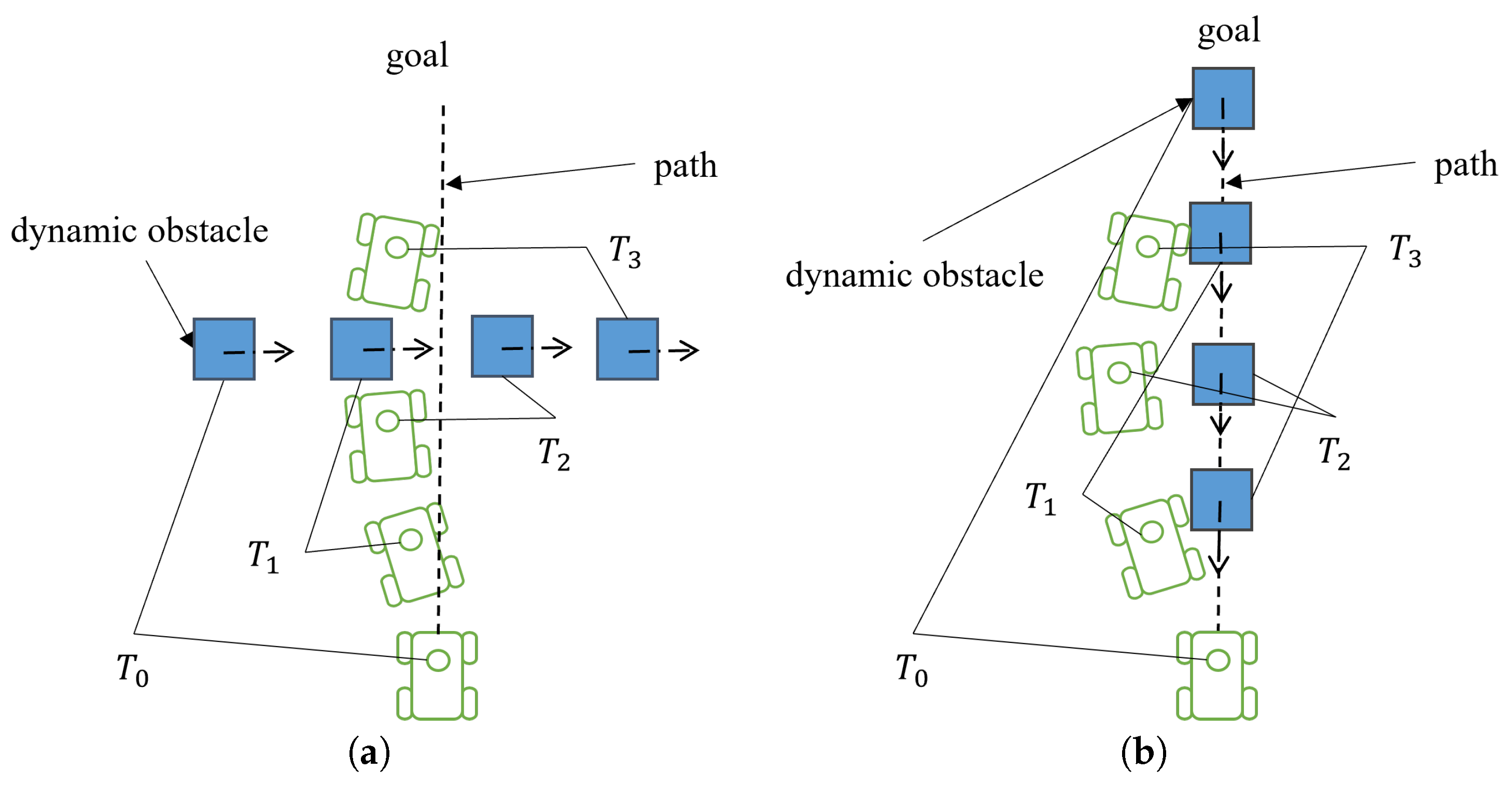
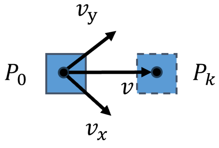
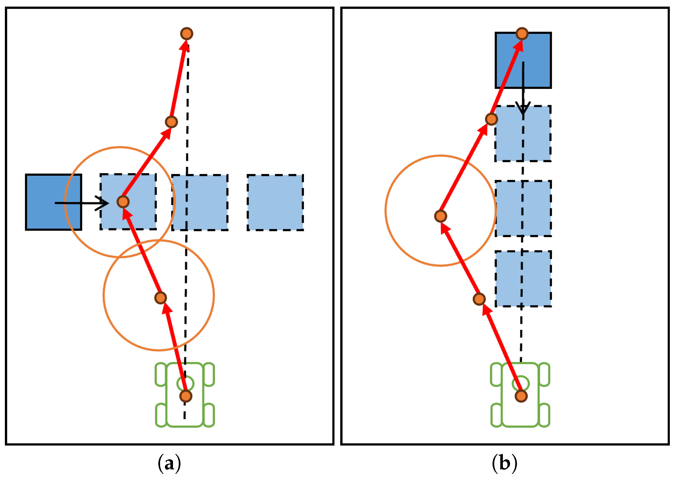
3.2. Improved TEB Algorithm

The TEB algorithm is a classic local path planning algorithm. Based on the elastic band (EB) algorithm, it adds various constraints such as time, velocities, obstacles, and path and robot kinematic constraints. It imagines the ideal path as a elastic band and treats all external constraints as external forces that cause the elastic band to deform. The original TEB algorithm obtains the location information of obstacles through a local cost map. Therefore, the information obtained by the algorithm does not include the motion information of the obstacles. This will cause the algorithm to perform poorly in an environment with dynamic obstacles, mainly due to the possibilities that there is no time to avoid obstacles and that the obstacle avoidance path is not optimal. Therefore, in order to optimize the operating effect of the algorithm in a dynamic environment, this article optimizes the path by associating the TEB poses and the obstacle positions at the corresponding future time. This article introduces a new constraint function:

$$f_{fpobs}=e\left(-d_{min,j},-r_{o_{min}},ϵ,S,n\right)$$

(14)

where $d_{min,j}$ is the distance between the TEB pose and the obstacle at the corresponding time, $r_{o_{min}}$ is the minimum distance between the obstacle and the pose point, and the specific expansion formula of the e function is as follows:

$$e(x,x_r,ϵ,S,n)\cong \left\{\begin{array}{cc}{\left(\frac{x-(x_r-ϵ)}{S}\right)}^n\hfill & x>x_r-ϵ\hfill \\ 0\hfill & else\hfill \end{array}\right.$$

(15)

where $x_r$ is the limit value, and S, n, and $ϵ$ affect the accuracy of the approximation and are scaling, polynomial order, and a small displacement around the approximation value, respectively.

The obstacle avoidance effects of the improved TEB algorithm when facing obstacles in different directions are shown in Figure 2. As can be seen from Figure 2a, when it is detected that the obstacle is moving from left to right, the improved TEB algorithm plans an obstacle avoidance path to avoid the obstacle to the left. The same is true for the obstacle avoidance in Figure 2b. As can be seen from the schematic diagram, when it detects that the direction of movement of an obstacle is towards the robot from top to bottom, the algorithm makes a decision to avoid obstacles in advance instead of waiting until the robot enters the area affected by the obstacle.

Figure 3 is a schematic diagram of the proposed obstacle position in the future. The position of the obstacle is related to the corresponding TEB pose, where the position of the j-th obstacle is $P_j={[x_j,y_j]}^T$, as follows:

$$P_j=P_0+\sum _{i=0}^j\left(V+d{t}_i^{i+1}+\frac{A\times {\left(d{t}_i^{i+1}\right)}^2}{2}\right),j\in [1,k]$$

(16)

where $V={[v_x,v_y]}^T$, $A={[a_x,a_y]}^T$ are the speed and acceleration, respectively, of the obstacle detected at the current moment, and $d{t}_i^{i+1}$ is the time interval between the i-th and ($i+1$)-th TEB poses.

Figure 4 shows the details of dynamic obstacle avoidance achieved by the improved TEB algorithm in Figure 2. It can be clearly seen from Figure 4a that at time $T_0$, the robot has planned a path to avoid obstacles to the left, because at this time, the obstacle corresponding to the second TEB pose is on the ideal path of the robot, so the TEB pose at this position will be stretched to the left. Due to the characteristics of the TEB poses, the TEB poses adjacent to it will also be affected and stretched to the left. The robot will move to the left and avoid obstacles. The same applies to the poses in Figure 4b.

It can be seen from the above that the improved TEB algorithm can combine the TEB poses with the future positions of obstacles and plan a local path that integrates the obstacle velocities, improving the obstacle avoidance efficiency of the mobile robot when facing dynamic obstacles. In order to verify the proposed algorithm’s effectiveness, this article will verify the algorithm on simulation and experimental platforms.

4. Simulations and Experiments

4.1. Simulations

The simulation environment has good repeatability and controllable conditions. To evaluate the robustness and efficacy of the proposed approach in a dynamic environment, we use Gazebo and the ROS for simulations (the simulation environment is shown in Figure 5) and choose an Ackermann type of car as the mobile robot. First, we map the environment in a simulation environment without dynamic obstacles, and then, we add corresponding obstacles for simulation testing experiments. We use rosbag to extract the simulation data and then export the relevant topic information in the .bag file into a .csv file for analysis. We verify the navigation effect of the proposed method for a single obstacle with various velocities and directions and in a complex environment with multiple obstacles. For the first two simulations, to highlight our improvements over the original TEB local planner, we compare the navigation effect of the improved TEB with the effect of the original. In order to demonstrate the advantages of the proposed method over other local planners, we also compare the improved TEB with a model predictive control (MPC) local planner and a state lattice planner in the third simulation.

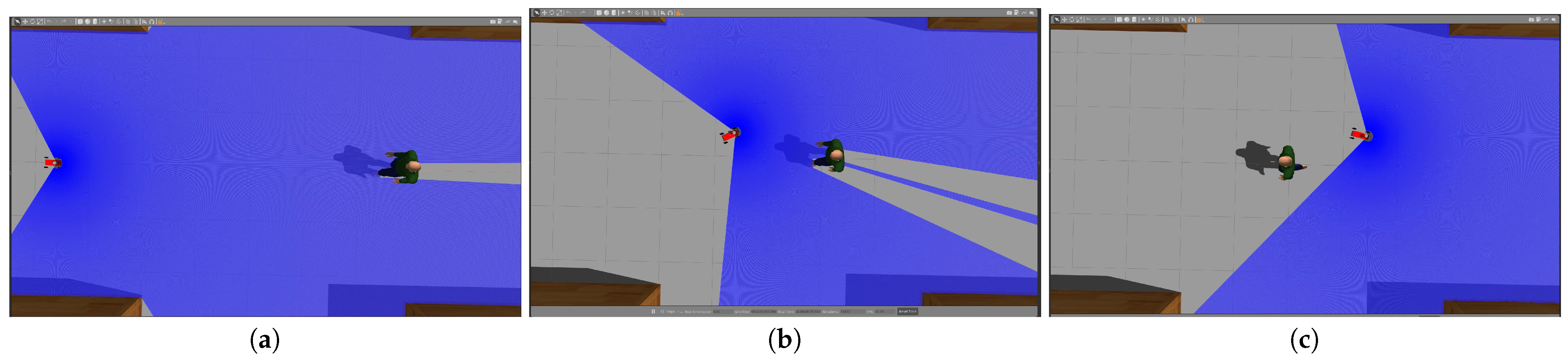
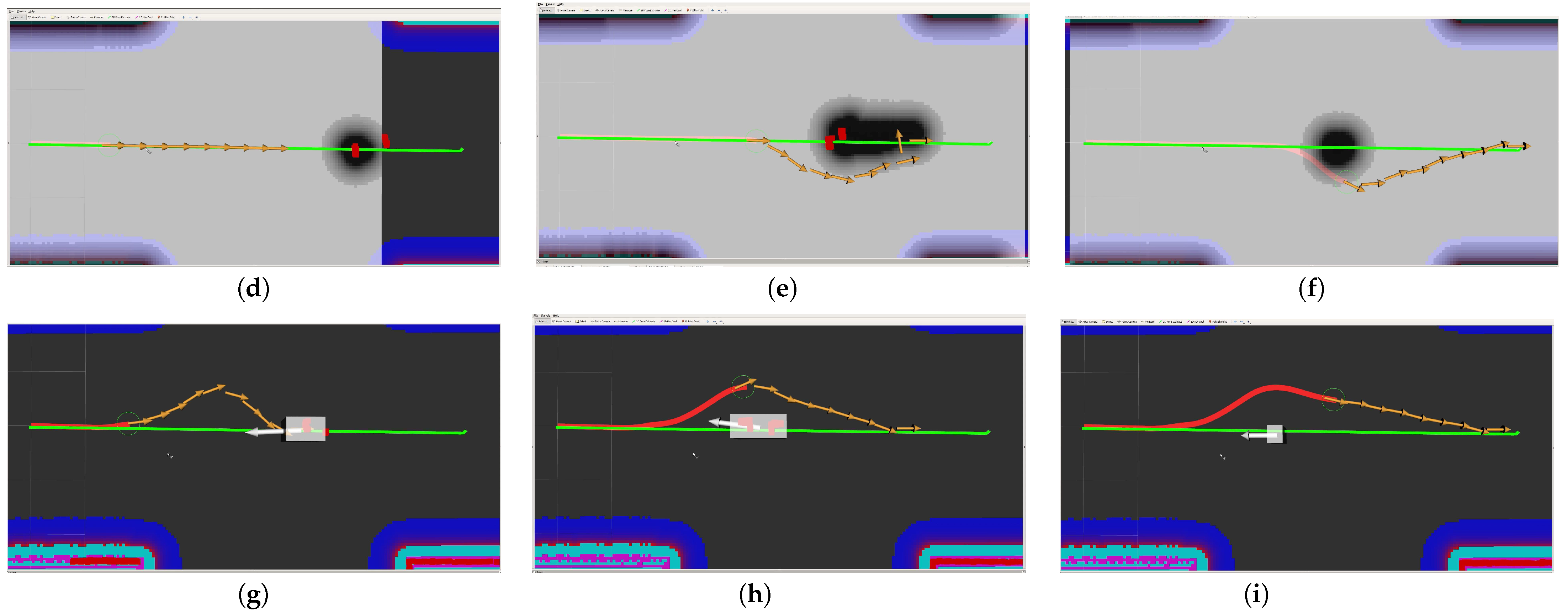
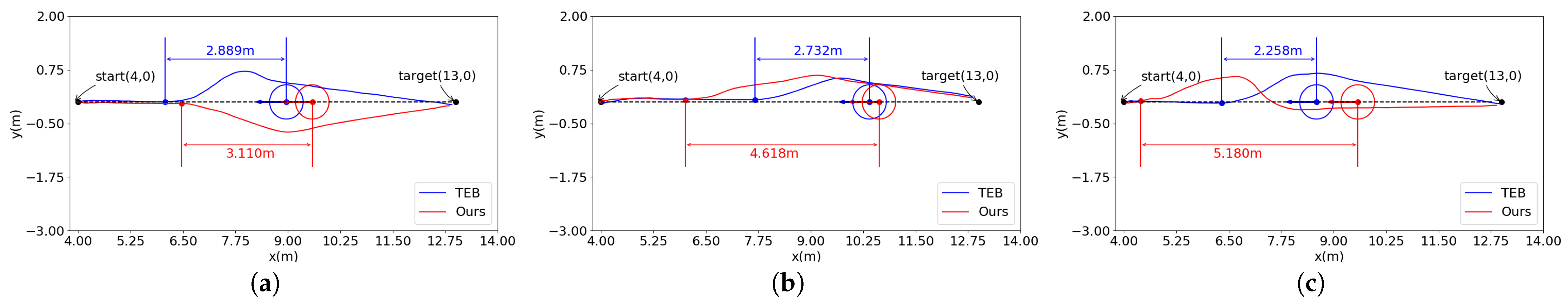
4.1.1. Obstacle Ahead of the Robot

The first set of simulations is used to verify the obstacle avoidance effect of the method for a single obstacle with different velocities coming from the front. The simulation environment is shown in the first row of Figure 6. The start position of the pedestrian is (12, 0), and the pedestrian moves at a speed of $0.8$ m/s, $1.0$ m/s, and $1.2$ m/s, respectively, in the three simulations. From the comparison of Figure 6d,g, it can be seen that the distance between the robot and the pedestrian is approximately 5 m at this time, but the TEB poses of the original algorithm are still in the reference path, while for our method, the robot predicts that in the future, a pedestrian will affect its trajectory, so advanced obstacle avoidance actions are taken.

From Figure 7, we can observe that the proposed method can perform obstacle avoidance behavior when the robot is at a considerable distance from the obstacle. When the robot takes obstacle avoidance actions, the distance between the robot and the obstacle is called the reaction distance. We computed the relationship between the reaction distance and the obstacle velocity and formed

Table 1. Relationship table between reaction distance and pedestrian velocity.

Pedestrian Velocity	TEB	Ours
0.8 m/s	2.998 m	3.110 m
1.0 m/s	2.732 m	4.618 m
1.2 m/s	2.258 m	5.180 m

. From Table 1, we can conclude that for the proposed method, the reaction distance is determined by the detected obstacle velocity, while for the original TEB, the reaction distance does not change much, or it even decreases in the case of encountering a faster obstacle—the robot may react too late to avoid obstacles. Therefore, it is necessary to take obstacle avoidance actions in advance. This simulation proves that the improved TEB can control the reaction distance to avoid obstacles in advance according to the velocities of obstacles.

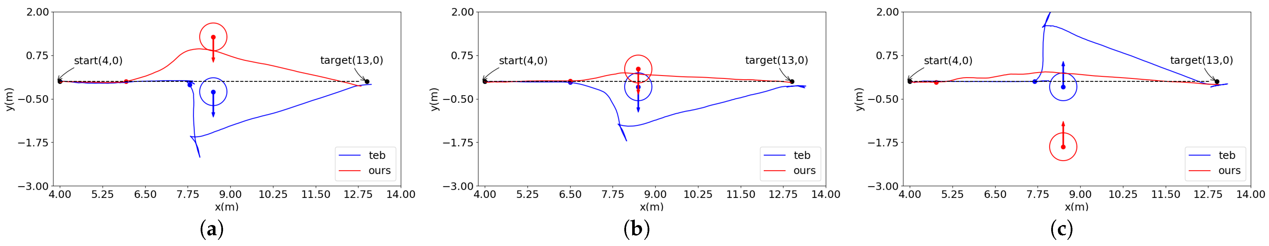
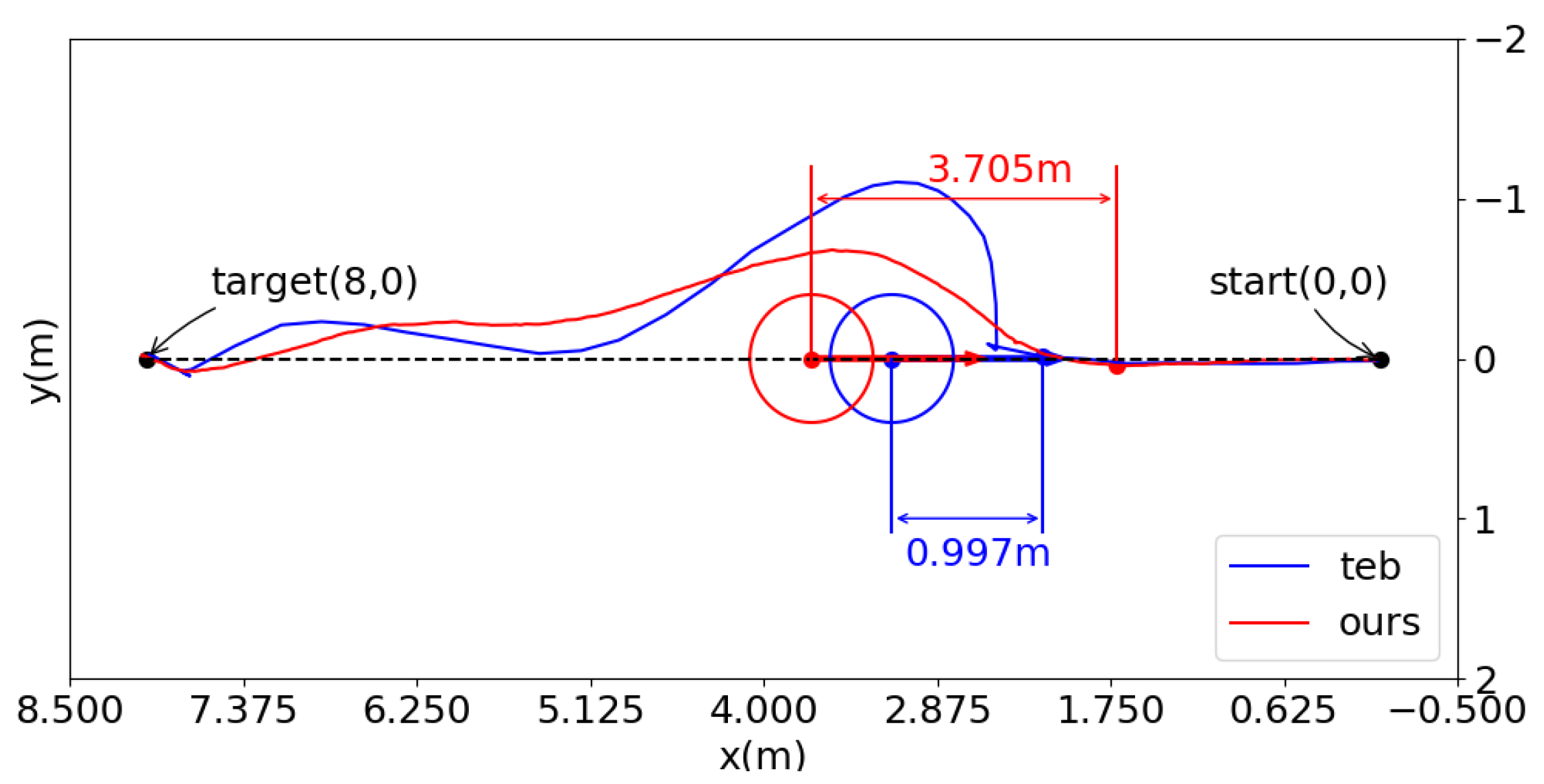
4.1.2. Obstacle Approaching from the Side of the Robot

The second simulation changes the direction of the pedestrian. The simulation environment is shown in Figure 8. The start and target of the robot remain unchanged, but the ideal path conflicts with pedestrians, forcing the robot to avoid them. We observe the obstacle avoidance effect of the robot. From the first row and the second row in Figure 8, we can clearly see that the robot runs at low efficiency under the original TEB. However, from Figure 8g–l, it can be seen that in the improved TEB, under the influence of the risk area, the robot adopts the strategy of avoiding obstacles to the left.

From the experimental effect in Figure 9a, we can see that, although the pedestrian does not block the robot at this time, the obstacle risk area affects the TEB poses. Therefore, the robot decides in advance to go in the opposite direction of the area where pedestrians are walking. The difference between Figure 9a,b lies in the initial position of the pedestrian when the robot starts. The position y of the pedestrian in Figure 9b is smaller than that in Figure 9a. The robot does not need to make too much of a left-turn deflection so that obstacles can be avoided using our method, and the original TEB also appears to move around obstacles. In Figure 9c, the direction of the pedestrian is from the negative direction of y to the positive direction. In the improved algorithm, when the position of the pedestrian is far away from the ideal trajectory of the robot, the robot takes a left turn to avoid obstacles in advance. However, the original TEB takes obstacle avoidance measures only when pedestrians almost collide with robots. The obstacle avoidance efficiency is low, and collisions are prone to occur. This set of simulations proves that the robot will choose the obstacle avoidance direction based on the direction of the pedestrians.

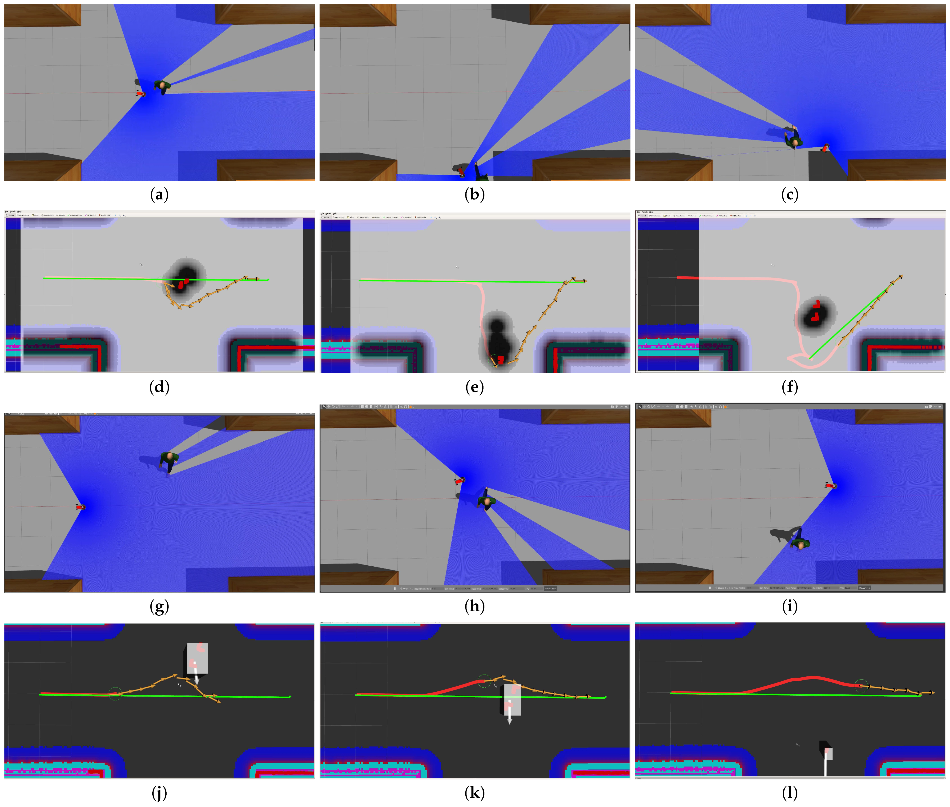
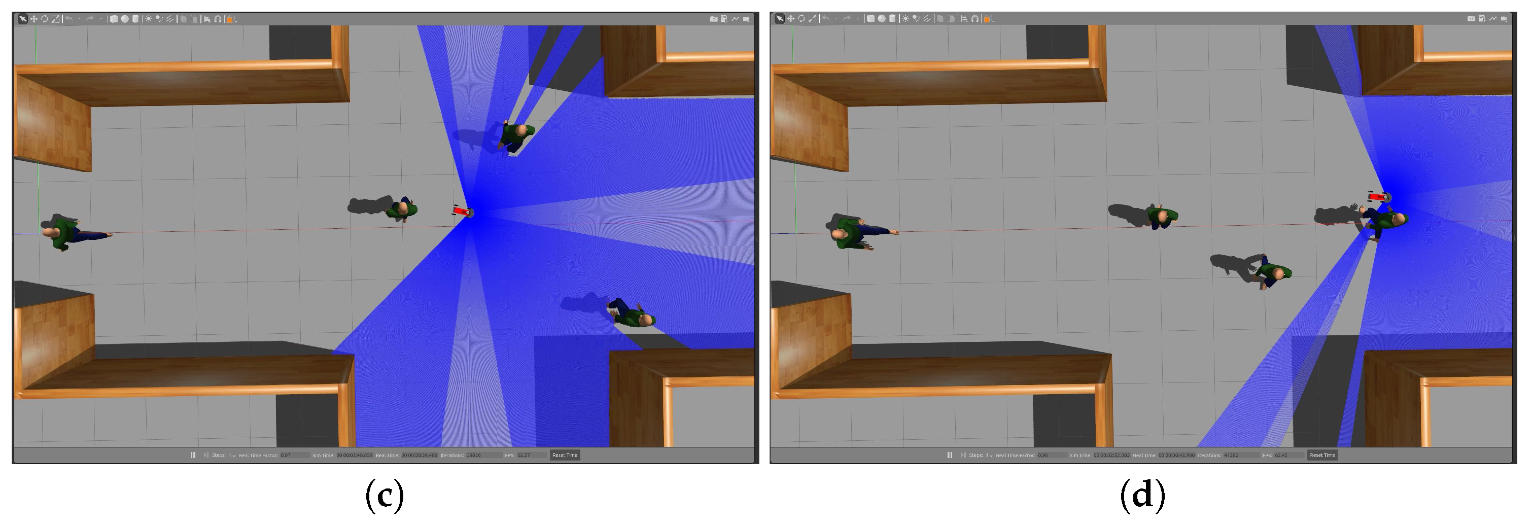
4.1.3. Navigation in Complex Environments

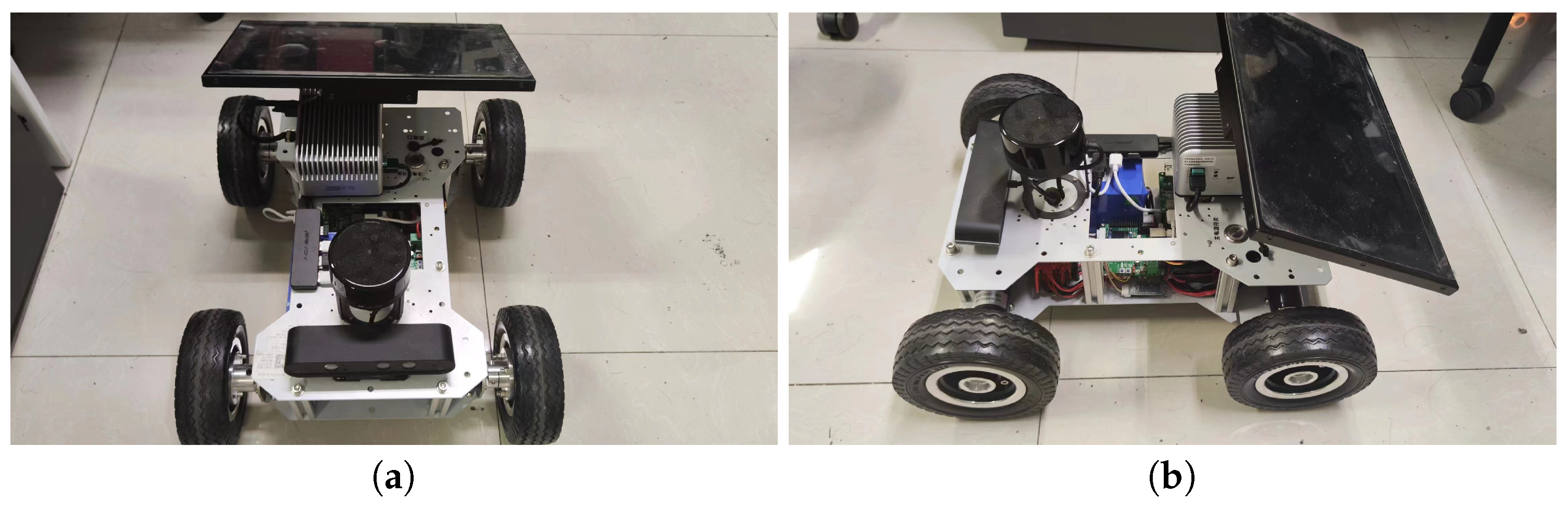
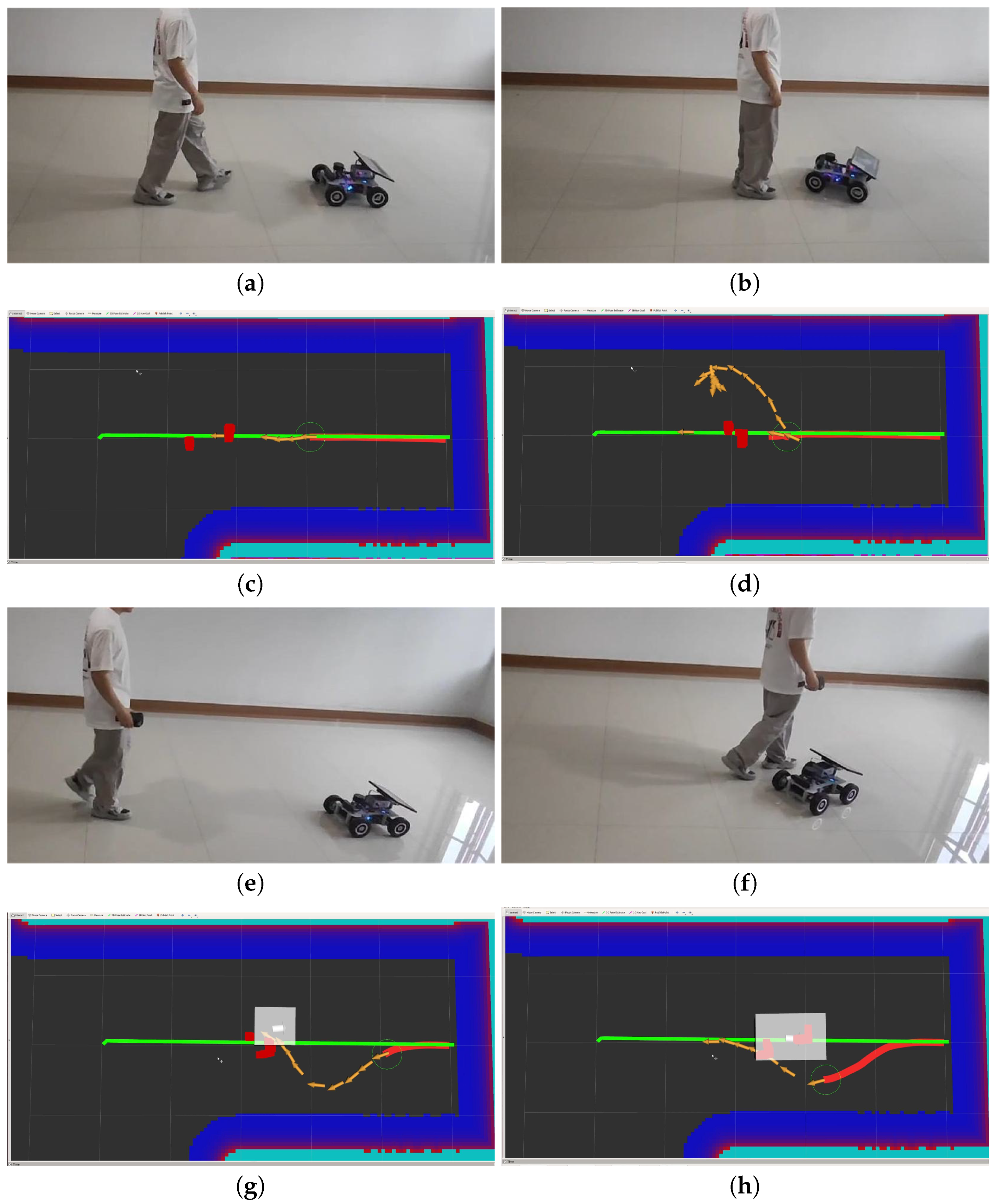
The third set of simulation experiments allowed the robot to run in a complex, multidynamic obstacle scene, as shown in Figure 10. Four pedestrians moved at a speed of $0.8$ m/s. We compare our method with the original TEB, the MPC local planner, and the state lattice planner in this section. For the four local planners, we conducted 50 simulation experiments. For the robot, it is considered successful if it reaches the target within the specified time, and it is considered to have failed if it collides or gets stuck on the path. Through the rosbag file, we performed some processing on the data to calculate the success rates, total running distances, and times of the four methods to form

Table 2. The success rates, running distances, and total times of the four methods.

Algorithm	Success	Running Distance	Time
TEB local planner	75%	18.61 m	21.81 s
MPC local planner	80%	17.54 m	21.62 s
State lattice	90%	16.33 m	18.82 s
Ours	95%	15.03 m	16.82 s

. We can see from Table 2 that the improved TEB not only improves the success rate of dynamic obstacle avoidance, but it also increases the average speed of the robot on the global path and reduces the running distance. Through this simulation, we found that the improved TEB is not only better than the original TEB, but it is also more effective than other advanced local planners.

4.2. Experiments

In order to verify the efficiency of the proposed method on an actual robot platform, we designed a mobile robot experimental platform. The platform includes a two-dimensional lidar for sensing the environment, and the lidar is connected to the upper computer: a Jetson Nano. The chassis is controlled by an STM32 to control the motor movement of the robot. Our method works under ROS-Melodic. The real environment experiment must be used to verify whether the robot uses obstacle avoidance operations for oncoming pedestrians in advance. As shown in Figure 11, the start of the given robot is $(0,0)$, and the target starts at $(8,0)$. When the robot starts, a person moves slowly toward the robot as a dynamic obstacle.

From Figure 12a–d in the original algorithm, when the pedestrian moves in front of the robot, since the position of the pedestrian does not affect the first few TEB poses, the robot still runs on the ideal trajectory. Only when the position of the pedestrian reaches a position close enough to the robot does the robot identify the obstacle and devise a trajectory to circumvent it. Because it is too close to the obstacle, there is an operation of turning in place. If the pedestrian does not notice the robot at this time, it may collide with the pedestrian. From Figure 12e–h, we can see that in the improved method, the robot performs maneuvering operations in advance when facing oncoming pedestrians: the position of the pedestrian in Figure 12g is the same as in Figure 12c, and the distance between the pedestrian and the robot is approximately the same or even greater, but the robot has already started to avoid obstacles in advance, so even if the pedestrian maintains his/her own trajectory at this time, the route of the robot can perfectly stagger with the pedestrian.

From the trajectory path diagram in Figure 13, we can see the difference between the two methods of advance obstacle avoidance more intuitively. The reaction distance of the original TEB is only approximately 1 m, while the reaction distance of the improved TEB algorithm is as high as $3.5$ m. The total running path of the robot in the original TEB is longer.

4.3. Discussion

Simulations and experiments show that the combination of obstacle velocities and TEB poses can improve the efficiency of dynamic obstacle avoidance. The first simulation verified that the improved TEB can plan different obstacle avoidance paths for obstacles with different velocities, the robot can avoid obstacle in advance based on the velocities of obstacles, and the reaction distance increases as the speed of the obstacles increases, which can ensure the safety of the robot while moving. The second simulation showed that our method can make different obstacle avoidance strategies for obstacles from different directions, which improves the efficiency of obstacle avoidance. The third simulation demonstrated the effectiveness of our method in environments with multiple dynamic obstacles, and we compared the improved TEB with other advanced local planners, including an MPC local planner and a state lattice planner. The comparative experiments with other planners showed that the improved TEB reduces the total running time and running distance and increases the success rate, proving that the improved TEB can indeed improve the efficiency of local path planning in dynamic environments. Finally, the robot platform experiment verified that our method can run on a robot platform and is better than the original TEB. Simulations and experiments prove the contribution of this article and the necessity of our research.

5. Conclusions

Due to the uncertainty of robot movement, dynamic obstacle avoidance poses many challenges to robot navigation. The traditional method of avoiding static obstacles is to set the inflation radius of obstacles or to increase the update frequency of the local cost map. However, the positions of dynamic obstacles change. These methods do not robustly consider the velocities of obstacles. If the speed of the obstacle is too fast, the robot may not have enough time to avoid the obstacle when it is too close to the obstacle. In this manuscript, we propose a new dynamic obstacle avoidance method that detects and estimates the velocities of dynamic obstacles through 2D lidar and integrates the TEB local planner. We conduct simulations and real experiments to demonstrate that the proposed method can perform advanced avoidance according to the velocity of obstacles, but this algorithm is more dependent on the accuracy of the localization algorithm. In the future, we plan to conduct further research on the uncertainty of the directions of dynamic obstacles.

References

1. Qi, J.; Yang, H.; Sun, H. MOD-RRT*: A sampling-based algorithm for robot path planning in dynamic environment. IEEE Trans. Ind. Electron. 2020, 68, 7244–7251. [Google Scholar] [CrossRef]
2. Zhang, Y.; Wang, S. LSPP: A novel path planning algorithm based on perceiving line segment feature. IEEE Sens. J. 2021, 22, 720–731. [Google Scholar] [CrossRef]
3. Kim, B.; Pineau, J. Socially adaptive path planning in human environments using inverse reinforcement learning. Int. J. Soc. Robot. 2016, 8, 51–66. [Google Scholar] [CrossRef]
4. Sun, T.; Pan, W.; Wang, Y.; Liu, Y. Region of interest constrained negative obstacle detection and tracking with a stereo camera. IEEE Sens. J. 2022, 22, 3616–3625. [Google Scholar] [CrossRef]
5. Almasri, M.M.; Alajlan, A.M.; Elleithy, K.M. Trajectory planning and collision avoidance algorithm for mobile robotics system. IEEE Sens. J. 2016, 16, 5021–5028. [Google Scholar] [CrossRef]
6. Kobayashi, Y.; Sugimoto, T.; Tanaka, K.; Shimomura, Y.; Arjonilla Garcia, F.J.; Kim, C.H.; Yabushita, H.; Toda, T. Robot navigation based on predicting of human interaction and its reproducible evaluation in a densely crowded environment. Int. J. Soc. Robot. 2022, 14, 373–387. [Google Scholar] [CrossRef]
7. Duong, H.T.; Suh, Y.S. Human gait tracking for normal people and walker users using a 2D LiDAR. IEEE Sens. J. 2020, 20, 6191–6199. [Google Scholar] [CrossRef]
8. Lee, H.; Lee, H.; Shin, D.; Yi, K. Moving objects tracking based on geometric model-free approach with particle filter using automotive LiDAR. IEEE Trans. Intell. Transp. Syst. 2022, 23, 17863–17872. [Google Scholar] [CrossRef]
9. Wei, C.; Wang, Y.; Shen, Z.; Xiao, D.; Bai, X.; Chen, H. AUQ–ADMM algorithm-based peer-to-peer trading strategy in large-scale interconnected microgrid systems considering carbon trading. IEEE Syst. J. 2023, 17, 6248–6259. [Google Scholar] [CrossRef]
10. Chen, Q.; Li, Y.; Hong, Y.; Shi, H. Prescribed-Time Robust Repetitive Learning Control for PMSM Servo Systems. IEEE Trans. Ind. Electron. 2024; in press. [Google Scholar] [CrossRef]
11. Shim, I.; Choi, D.G.; Shin, S.; Kweon, I.S. Multi lidar system for fast obstacle detection. In Proceedings of the 2012 9th International Conference on Ubiquitous Robots and Ambient Intelligence (URAI), Daejeon, Republic of Korea, 26–28 November 2012; IEEE: Piscataway, NJ, USA, 2012; pp. 557–558. [Google Scholar]
12. Fox, D.; Burgard, W.; Thrun, S. The dynamic window approach to collision avoidance. IEEE Robot. Autom. Mag. 1997, 4, 23–33. [Google Scholar] [CrossRef]
13. Rösmann, C.; Feiten, W.; Wösch, T.; Hoffmann, F.; Bertram, T. Trajectory modification considering dynamic constraints of autonomous robots. In Proceedings of the ROBOTIK 2012: 7th German Conference on Robotics, VDE, Munich, Germany, 21–22 May 2012; pp. 1–6. [Google Scholar]
14. Rösmann, C.; Hoffmann, F.; Bertram, T. Planning of multiple robot trajectories in distinctive topologies. In Proceedings of the 2015 European Conference on Mobile Robots (ECMR), Lincoln, UK, 2–4 September 2015; IEEE: Piscataway, NJ, USA, 2015; pp. 1–6. [Google Scholar]
15. Rösmann, C.; Hoffmann, F.; Bertram, T. Kinodynamic trajectory optimization and control for car-like robots. In Proceedings of the 2017 IEEE/RSJ International Conference on Intelligent Robots and Systems (IROS), Vancouver, BC, Canada, 24–28 September 2017; IEEE: Piscataway, NJ, USA, 2017; pp. 5681–5686. [Google Scholar]
16. Rösmann, C.; Oeljeklaus, M.; Hoffmann, F.; Bertram, T. Online trajectory prediction and planning for social robot navigation. In Proceedings of the 2017 IEEE International Conference on Advanced Intelligent Mechatronics (AIM), Munich, Germany, 3–7 July 2017; IEEE: Piscataway, NJ, USA, 2017; pp. 1255–1260. [Google Scholar]
17. Rösmann, C.; Feiten, W.; Wösch, T.; Hoffmann, F.; Bertram, T. Efficient trajectory optimization using a sparse model. In Proceedings of the 2013 European Conference on Mobile Robots, Barcelona, Spain, 25–27 September 2013; IEEE: Piscataway, NJ, USA, 2013; pp. 138–143. [Google Scholar]
18. Hwang, C.L.; Huang, H.H. Experimental validation of a car-like automated guided vehicle with trajectory tracking, obstacle avoidance, and target approach. In Proceedings of the IECON 2017—43rd Annual Conference of the IEEE Industrial Electronics Society, Beijing, China, 29 October–1 November 2017; IEEE: Piscataway, NJ, USA, 2017; pp. 2858–2863. [Google Scholar]
19. Ding, Z.; Liu, J.; Chi, W.; Wang, J.; Chen, G.; Sun, L. PRTIRL based socially adaptive path planning for mobile robots. Int. J. Soc. Robot. 2023, 15, 129–142. [Google Scholar] [CrossRef]
20. Zhou, Y.; Tuzel, O. Voxelnet: End-to-end learning for point cloud based 3D object detection. In Proceedings of the IEEE Conference on Computer Vision and Pattern Recognition, Salt Lake City, UT, USA, 19–23 June 2018; pp. 4490–4499. [Google Scholar]
21. Ren, W.; Wang, X.; Tian, J.; Tang, Y.; Chan, A.B. Tracking-by-counting: Using network flows on crowd density maps for tracking multiple targets. IEEE Trans. Image Process. 2020, 30, 1439–1452. [Google Scholar] [CrossRef]
22. Li, C.; Guo, S.; Guo, J. Study on obstacle avoidance strategy using multiple ultrasonic sensors for spherical underwater robots. IEEE Sens. J. 2022, 22, 24458–24470. [Google Scholar] [CrossRef]
23. Jha, B.; Turetsky, V.; Shima, T. Robust path tracking by a Dubins ground vehicle. IEEE Trans. Control Syst. Technol. 2018, 27, 2614–2621. [Google Scholar] [CrossRef]
24. Sun, C.; Zhang, X.; Zhou, Q.; Tian, Y. A model predictive controller with switched tracking error for autonomous vehicle path tracking. IEEE Access 2019, 7, 53103–53114. [Google Scholar] [CrossRef]
25. Qu, P.; Li, S.; Zhang, J.; Duan, Z.; Mei, K. A Low-cost and Robust Mapping and Relocalization Method Base on Lidar Inertial Odometry. In Proceedings of the 2021 IEEE International Conference on Real-time Computing and Robotics (RCAR), Xining, China, 15–19 July 2021; IEEE: Piscataway, NJ, USA, 2021; pp. 257–262. [Google Scholar]
26. Wang, E.; Chen, D.; Fu, T.; Ma, L. A Robot Relocalization Method Based on Laser and Visual Features. In Proceedings of the 2022 IEEE 11th Data Driven Control and Learning Systems Conference (DDCLS), Chengdu, China, 3–5 August 2022; IEEE: Piscataway, NJ, USA, 2022; pp. 519–524. [Google Scholar]
27. Chen, X.; Vizzo, I.; Läbe, T.; Behley, J.; Stachniss, C. Range image-based LiDAR localization for autonomous vehicles. In Proceedings of the 2021 IEEE International Conference on Robotics and Automation (ICRA), Xian, China, 30 May–5 June 2021; IEEE: Piscataway, NJ, USA, 2021; pp. 5802–5808. [Google Scholar]
28. Welch, G.; Bishop, G. An Introduction to the Kalman Filter. 1995. Available online: https://perso.crans.org/club-krobot/doc/kalman.pdf (accessed on 20 April 2024).
29. Huang, Y.; Ding, H.; Zhang, Y.; Wang, H.; Cao, D.; Xu, N.; Hu, C. A motion planning and tracking framework for autonomous vehicles based on artificial potential field elaborated resistance network approach. IEEE Trans. Ind. Electron. 2019, 67, 1376–1386. [Google Scholar] [CrossRef]
30. Fiorini, P.; Shiller, Z. Motion planning in dynamic environments using velocity obstacles. Int. J. Robot. Res. 1998, 17, 760–772. [Google Scholar] [CrossRef]
31. Bharath, G.; Singh, A.; Kaushik, M.; Krishna, K.; Manocha, D. Prvo: Probabilistic reciprocal velocity obstacle for multi robot navigation under uncertainty. In Proceedings of the 2017 IEEE/RSJ International Conference on Intelligent Robots and Systems (IROS), Vancouver, BC, Canada, 24–28 September 2017; pp. 24–28. [Google Scholar]
32. Van den Berg, J.; Lin, M.; Manocha, D. Reciprocal velocity obstacles for real-time multi-agent navigation. In Proceedings of the 2008 IEEE International Conference on Robotics and Automation, Pasadena, CA, USA, 19–23 May 2008; IEEE: Piscataway, NJ, USA, 2008; pp. 1928–1935. [Google Scholar]
33. Guo, K.; Wang, D.; Fan, T.; Pan, J. VR-ORCA: Variable responsibility optimal reciprocal collision avoidance. IEEE Robot. Autom. Lett. 2021, 6, 4520–4527. [Google Scholar] [CrossRef]
34. Guo, B.; Guo, N.; Cen, Z. Obstacle avoidance with dynamic avoidance risk region for mobile robots in dynamic environments. IEEE Robot. Autom. Lett. 2022, 7, 5850–5857. [Google Scholar] [CrossRef]
35. Reddy, A.K.; Malviya, V.; Kala, R. Social cues in the autonomous navigation of indoor mobile robots. Int. J. Soc. Robot. 2021, 13, 1335–1358. [Google Scholar] [CrossRef]
36. Smith, T.; Chen, Y.; Hewitt, N.; Hu, B.; Gu, Y. Socially aware robot obstacle avoidance considering human intention and preferences. Int. J. Soc. Robot. 2021, 15, 661–678. [Google Scholar] [CrossRef]
37. Chen, C.S.; Lin, S.Y. Costmap generation based on dynamic obstacle detection and velocity obstacle estimation for autonomous mobile robot. In Proceedings of the 2021 21st International Conference on Control, Automation and Systems (ICCAS), Jeju, Republic of Korea, 12–15 October 2021; IEEE: Piscataway, NJ, USA, 2021; pp. 1963–1968. [Google Scholar]
38. Lu, D.V.; Hershberger, D.; Smart, W.D. Layered costmaps for context-sensitive navigation. In Proceedings of the 2014 IEEE/RSJ International Conference on Intelligent Robots and Systems, Chicago, IL, USA, 14–18 September 2014; IEEE: Piscataway, NJ, USA, 2014; pp. 709–715. [Google Scholar]
39. Wojke, N.; Bewley, A.; Paulus, D. Simple online and realtime tracking with a deep association metric. In Proceedings of the 2017 IEEE International Conference on Image Processing (ICIP), Beijing, China, 17–20 September 2017; IEEE: Piscataway, NJ, USA, 2017; pp. 3645–3649. [Google Scholar]
40. Dong, H.; Weng, C.Y.; Guo, C.; Yu, H.; Chen, I.M. Real-time avoidance strategy of dynamic obstacles via half model-free detection and tracking with 2d lidar for mobile robots. IEEE/ASME Trans. Mechatronics 2020, 26, 2215–2225. [Google Scholar] [CrossRef]
41. Wang, C.; Chen, X.; Li, C.; Song, R.; Li, Y.; Meng, M.Q.H. Chase and track: Toward safe and smooth trajectory planning for robotic navigation in dynamic environments. IEEE Trans. Ind. Electron. 2022, 70, 604–613. [Google Scholar] [CrossRef]
Figure 1. Schematic diagram of background point clustering. The points in the figure are the filtered obstacle points: the white points are the noise points, the black rectangle is the obstacle, and the blue area is the inflated obstacle area.
Processes 12 00984 g001
Figure 2. The dynamic obstacle avoidance effect of improved TEB: The green car represents the position of the mobile robot at different times, and the blue rectangle represents the position of the one obstacle at different times. The arrow represents the speed and direction of the obstacle. The robot’s target is at the top of the figure. The black dotted line is the ideal motion trajectory of the robot, with T 0 T 3 indicating time 0 to time 3. (a) Obstacle from the side. (b) Obstacle from the front.
Processes 12 00984 g002
Figure 3. Schematic diagram of the obstacle’s future position. The solid square area in the figure is the obstacle information detected at the current moment. It has component velocities in the x- and y-directions. The dotted line area is the k-th TEB pose.
Processes 12 00984 g003
Figure 4. Details of improved TEB. This figure presents the details at time T 0 . The local pose sequence of the robot in the figure consists of four red arrows, and the blue square is the obstalce at T 0 while the light-blue squares are the future positions of the obstalce at different times. And the green car represents the robot. The specific calculation process can be referenced in Figure 3 and Equation (16).
Processes 12 00984 g004
Figure 5. Simulation environment: (a) the simulation environment, which is a cross corridor, (b) the car used in the simulation, (c) the pedestrian acting as a dynamic obstacle in the simulation. The blue area in the figure represents the area that the lidar can scan.
Processes 12 00984 g005
Figure 6. Simulation processions: (ac) Gazebo snapshots of the robot’s avoidance maneuver when confronted with a pedestrian moving at a speed of 1.0 m/s. (di) Robot Visualization Tools (rviz) screenshots at different times for the original algorithm and our method; these figures display the robot’s global reference path, local path, history path, TEB poses, etc. In these figures, the yellow arrows represent the TEB poses; they can also be seen to be the positions that the robot will reach in the future. The red point cloud is the obstacle point cloud, the green path is the global reference path, the red trajectory represents the robot’s history path, and the white binding box is the detected obstacle.
Processes 12 00984 g006aProcesses 12 00984 g006b
Figure 7. (ac) Trajectories of the robot for pedestrian speeds of 0.8 m/s, 1.0 m/s, and 1.2 m/s, where the blue line is the original TEB, the red line is our method, and the circles are the positions of the pedestrian when the robot performs obstacle avoidance behavior under different algorithms. The position of the robot at this time is represented by red and blue solid dots, and the reaction distance is calculated and marked with numbers with different colors in the figure.
Processes 12 00984 g007
Figure 8. (ac,gi) Snapshots of the robot using the original TEB and our method to avoid side pedestrians. (df,jl) The rviz screenshots during the operation of the original TEB and our method, respectively, in which the yellow arrows are the TEB poses.
Processes 12 00984 g008
Figure 9. (ac) Experimental results of the robot in three different situations. The three different situations here are aimed at different moments when the three robots are started. The blue line is the original algorithm, the red line is the proposed algorithm, and the circle represents the positions of the pedestrian when the robot is performing obstacle avoidance behavior. At this time, the position of the robot is marked with red and blue solid circles.
Processes 12 00984 g009
Figure 10. Snapshots of the robot using the improved method to avoid obstacles in a complex, dynamic simulation environment. (ad) the different time during the simulation.
Processes 12 00984 g010aProcesses 12 00984 g010b
Figure 11. (a) the front view of the robot platform, (b) the side view.
Processes 12 00984 g011
Figure 12. Photos of the robot facing oncoming pedestrians and the corresponding rviz screenshots. The yellow arrow indicates the TEB poses, and the red point cloud is the pedestrian scanned by the 2D lidar: (ad) the original TEB, and (eh) our method.
Processes 12 00984 g012
Figure 13. Trajectories of two methods.
Processes 12 00984 g013