Study on the Dynamic Characteristics of Single Cavitation Bubble Motion near the Wall Based on the Keller–Miksis Model

Abstract

The dynamic model of cavitation bubbles serves as the foundation for the study of all cavitation phenomena. Solving the cavitation bubble dynamics equation can better elucidate the physical principles of bubble dynamics, assisting with the design of hydraulic machinery and fluid control. This paper employs a fourth-order explicit Runge–Kutta numerical method to solve the translational Keller–Miksis model for cavitation bubbles. It analyzes the collapse time, velocity, as well as the motion and force characteristics of bubbles under different wall distances γ values. The results indicate that as the distance between the cavitation bubble and the wall decreases, the cavitation bubble collapse time increases, the displacement of the center of mass and the amplitude of translational velocity of the cavitation bubble increase, and the minimum radius of the cavitation bubble gradually decreases linearly. During the stage when the cavitation bubble collapses to its minimum radius, the Bjerknes force and resistance experienced by the bubble also increase as the distance to the wall decreases. Especially in the cases where γ = 1.3 and 1.5, during the rebound stage of the bubble, the Bjerknes force and resistance increase, causing the bubble to move away from the wall. Meanwhile, this study proposes a radiation pressure coefficient to characterize the radial vibration behavior of cavitation bubbles when analyzing the radiation sound pressure. It is found that the wall distance has a relatively minor effect on the radiation pressure coefficient, providing an important basis for future research on the effects of different scale bubbles and multiple bubbles. The overall idea of this paper is to numerically solve the bubble dynamics equation, explore the characteristics of bubble dynamics, and elucidate the specific manifestations of physical quantities that affect bubble motion. This provides theoretical references for further engineering applications and flow analysis.

1. Introduction

Since Euler proposed cavitation [1] in 1753, how to reduce the occurrence of cavitation has become a worldwide problem in the field of hydraulic machinery and marine engineering. It has also been the research subject in many fields such as hydromechanics, fluid dynamics, and ocean engineering. The research on the dynamics of cavitation bubble is divided into theoretical analysis, experimental studies, and numerical calculations, Theoretical analysis elucidates the dynamic properties of cavitation bubble and their interaction with surrounding fluids, facilitating a deeper understanding of their movement mechanisms. This provides essential theoretical guidance for experimental design and numerical simulations.

In 1917, Rayleigh [2] first modeled the dynamics of a spherical cavitation bubble under ideal fluid conditions employing the ideal gas equation of state, and initially mathematically described the collapse of a cavitation bubble in an infinite flow field. However, due to the liquid surface tension and viscosity are not considered, when the cavitation bubble shrinks to the minimum radius, the vacuole collapse velocity and acceleration will tend to infinity, and there is no rebound phenomenon, which is obviously inconsistent with the reality. In 1949, Plesset [3] modified the Rayleigh model by adding a liquid surface tension term and a viscous force term to derive the classical Rayleigh–Plesset (R-P) equation for vacuole oscillations in incompressible flows, and experimentally verified that the model is accurate for most of the time of cavitation bubble growth and collapse. However, the Rayleigh–Plesset model, by disregarding the compressibility of the liquid, exhibits significant deviations from experimental observations during the late stages of collapse. Later in 1952, through the Kirkwood–Bethe assumption, Gilmore [4] and others further modified the Rayleigh model by taking into account the weak compressibility of the liquid, which later became known as the Gilmore model, the model lays the foundation for the subsequent collapse of cavitation bubble incompressible fluids. In 1980, Keller and Miksis [5] derived the Keller–Miksis cavitation bubble dynamics model that can describe the pulsation characteristics of a spherical cavitation bubble in an acoustic field based on the incompressible Bernoulli equation and the fluctuation equation, taking into account the effects of the acoustic radiation effect, incident acoustic waves, liquid viscosity, surface tension, and the compressibility of the liquid. Subsequently, a large number of scholars, such as Sochard [6], Ida [7], Kiyokami [8], and others, have embarked on studying the kinetic model of single cavitation bubbles, double cavitation bubbles, and groups of vacuoles in the near-wall region. They have augmented the Keller–Miksis model by incorporating an interaction term between bubbles. Meanwhile, Blake and Best [9] formulated the Kelvin impulse theory of bubbles, focusing on fluid momentum. This theory offers insights into the non-spherical deformation of vacuoles near boundaries, jet generation, and bubble behavior under various flow field boundary conditions, rendering it widely applicable. Their research has opened up new approaches to exploring cavitation bubble-wall interactions and led to a great breakthrough.

The cavitation bubble dynamics model is a second-order nonlinear ordinary differential equation. Due to its strong nonlinear nature, obtaining an analytical solution for the bubble radius as a function of time is challenging. This difficulty hinders understanding the characteristics of bubble motion from a physical perspective and limits its practical engineering theoretical guidance. With the rapid development of computer technology and image processing [10,11,12,13], we now can numerically solve these complex differential equations using numerical methods. In this paper, we utilized the Runge–Kutta numerical method to obtain the numerical solution of the bubble dynamics model. Through the combined analysis of the Keller–Miksis model and the bubble translational motion equation, we obtained the variation patterns of the bubble radius and velocity over time. Additionally, we further investigated the translational motion of the bubble under different wall distances γ and its mechanical characteristics. This study holds significant theoretical implications for understanding the dynamic behavior of bubbles under different coupling conditions and their relevant mechanical properties. It provides scientific guidance for the fields related to cavitation bubbles that are widely applied in scientific research and engineering practices.

2. Theoretical Background and Numerical Methods

2.1. Cavitation Bubble Dynamics Model

Keller and Miksis [14] augmented the Rayleigh–Plesset equation with acoustic assumptions, taking into account not only the influence of vapor pressure inside the cavitation bubble, liquid viscosity, and surface tension, but also acoustic radiation effects and the compressibility of the liquid. Additionally, they introduced a delay time term of t + R/c during the cavitation bubble collapse process, resulting in the Keller–Miksis model:

$$\left(1-\frac{\dot{R}}{c}\right)\dot{R}\ddot{R}+\left(\frac{3}{2}-\frac{\dot{R}}{2c}\right){\dot{R}}^2=\frac{1}{\rho }\left(1+\frac{\dot{R}}{c}\right)\left(p_l-p_{\infty }\left(t\right)\right)+\frac{R}{\rho c}\frac{d}{dt}{p}_l$$

(1)

In the equations, $\dot{R}$ represents dR/dt, $R$ is the radius of the cavitation bubble, $\dot{R}$ denotes the velocity of the bubble wall, $\ddot{R}$ denotes the acceleration of the bubble wall, c represents the speed of sound in the liquid, ρ is the density of the liquid, $p_{\infty }(t)$ signifies the ambient pressure at infinity, $p_l$ represents the pressure at the bubble wall, which can be calculated using the following formula:

$$p_l=p_{G0}{\left(\frac{R_0}{R}\right)}^{3\kappa }-\frac{4{\upsilon }_L\dot{R}}{R}-\frac{2S}{\rho R}$$

(2)

where p_G0 represents the partial pressure of the non-condensable gas, with gas properties exhibiting exponential variation. The effects of thermal effects are neglected, and there is no mass transfer between the gas and liquid phases. ${\upsilon }_L$ denotes the dynamic viscosity coefficient of the liquid, $S$ stands for surface tension, and $\kappa$ represents the polytropic index of the gas. When c approaches infinity, the weakly compressible Keller–Miksis model (1) can be simplified to the incompressible Rayleigh–Plesset model.

Adding the aforementioned cavitation bubble interaction terms to the Keller–Miksis model (Equation (1)), we obtain the Keller–Miksis equations the translational motion of the cavitation bubble [5,15,16]:

$$\left(1-\frac{{\dot{R}}_i}{c}\right){\dot{R}}_i{\ddot{R}}_i+\left(\frac{3}{2}-\frac{{\dot{R}}_i}{2c}\right){\dot{R}}_i{\hspace{0.17em}}^2=\frac{1}{\rho }\left(1+\frac{{\dot{R}}_i}{c}\right)\left(p_l-p_{\infty }\left(t\right)\right)+\frac{R_i}{\rho c}\frac{d}{dt}{p}_l-\frac{1}{d_{ij}}({\ddot{R}}_j{R}_j^2+2R_j{\dot{R}}_j^2)$$

(3)

The last term in Equation (11) represents the interaction between the primary bubble and the mirrored cavitation bubble. This model is derived from the Keller–Miksis model and describes the dynamics of two cavitation bubbles. It can be utilized to calculate the interaction between the cavitation bubble and the wall under different initial boundary conditions.

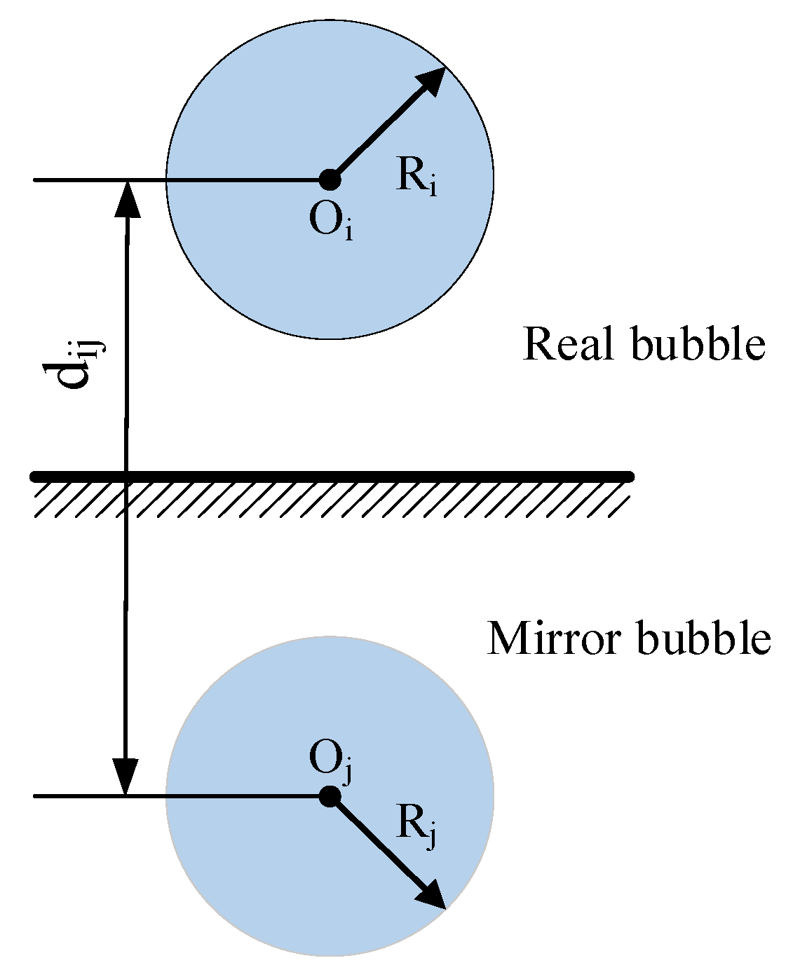
2.2. Translational Motion Equations of Near-Wall Cavitation Bubble

The movement of bubbles near the wall is mainly caused by the asymmetry of the boundary, leading to asymmetrical flow patterns around the bubble along the normal direction of the wall. This results in uneven forces acting on the bubble during collapse and implosion, causing it to move towards the wall and distort, ultimately rupturing to form microjets, thereby causing damage and destruction to the wall surface.

In this paper, the motion of bubbles near the wall is simplified into a problem of inviscid and irrotational two-dimensional potential flow. And it is assumed that there exists a mirrored cavitation bubble relative to the wall, with the cavitation bubble undergoing only vertical translational motion perpendicular to the wall. As shown in Figure 1, O_i represents the center of the primary bubble, while O_j represents the center of the mirrored bubble. In the subsequent formula derivations, i and j, respectively, denote the primary cavitation bubble and the mirrored cavitation bubble, with the outward normal direction of the wall defined as the positive direction.

Due to the close relationship between the object’s motion and the forces acting upon it, according to Newton’s second law, the equation of motion for the cavitation bubble is expressed as [14]:

$${\overrightarrow{F}}_i=\frac{d}{dt}\left(M_i{\overrightarrow{v}}_i\right)$$

(4)

In the equation, M_i represents the added mass matrix, and ${\overrightarrow{v}}_i$ denotes the translational velocity of the cavitation bubble. The added mass of the bubble near the wall is calculated using the following formula [15]:

$$M_i=K_i\frac{4}{3}\pi \rho R_i{\hspace{0.17em}}^3$$

(5)

where $K_i$ is equal to:

$$K_i=\frac{1}{2}\left(1+\frac{3}{8}\frac{R^3}{l^3}+\cdot \cdot \cdot \right)$$

(6)

where l represents the distance from the center of the bubble to the wall, since the distance l is greater than the bubble radius R, and the value of higher-order term $3R^3/8l^3$ is much smaller than 1. Additionally, this study does not consider the influence of micro-jets on the non-spherical deformation of the bubble. As a result, the bubble collapses spherically, and the off-diagonal elements of the additional mass matrix for a spherical bubble are all zero. Therefore, the term $3R^3/8l^3$ and higher-order terms can be ignored. When K_i = 0.5, the additional mass is equal to half of the displaced fluid mass. Now, substituting Equations (5) and (6) into Equation (4), we obtain:

$${\overrightarrow{F}}_i=\frac{2}{3}\pi \rho \frac{d}{dt}\left(R_i{\hspace{0.17em}}^3{\overrightarrow{v}}_i\right)$$

(7)

According to the studies of Mettin [16] and Moo J. G. S. [17], the forces acting on the cavitation bubble consist of secondary Bjerknes force and viscous drag:

$${\overrightarrow{F}}_i=\frac{2}{3}\pi \rho \frac{d}{dt}\left(R_i{\hspace{0.17em}}^3{\overrightarrow{v}}_i\right)={\overrightarrow{F}}_{B,i}+{\overrightarrow{F}}_{D,i}$$

(8)

$${\overrightarrow{F}}_{B,i}=\frac{\rho }{4\pi d_{ij}^2}{V}_i\frac{d^2{V}_j}{d{t}^2}\overrightarrow{e}=V_i\rho \frac{d}{dt}\left(R_j^2{\dot{R}}_j\right)=\frac{4}{3}\pi R_i^3\rho \left(2R_j{\dot{R}}_j^2+R_{{\hspace{0.17em}}_j}^2{\ddot{R}}_j\right)\frac{1}{d_{{\hspace{0.17em}}_{ij}}^2}\overrightarrow{e}$$

(9)

$${\overrightarrow{F}}_{D,i}=-12\pi {\upsilon }_L{R}_i{\overrightarrow{v}}_i$$

(10)

By rearranging Equation (8), we can derive the equation of motion for the translational motion of the cavitation bubble:

$${\overrightarrow{\dot{v}}}_i=\frac{1}{R_i{\hspace{0.17em}}^3}\left(\frac{3}{2\pi \rho }\left({\overrightarrow{F}}_{B,i}+{\overrightarrow{F}}_{D,i}\right)-3R_i^2{\dot{R}}_i{\overrightarrow{v}}_i\right)$$

(11)

2.3. Numerical Solution Methods

The numerical solution method employed in this paper is the fourth-order explicit Runge–Kutta method for solving the cavitation bubble dynamics model. The basic approach involves transforming the differential equations into a series of difference equations to progressively approximate the exact solution. Then, approximate solutions are obtained at discrete nodes. The computational formula for the fourth-order Runge–Kutta method is as follows [18,19]:

$$\left\{\begin{array}{l}{y}_{n+1}=y_n+\frac{h}{6}(k_1+2k_2+2k_3+k_4)\\ k_1=f(t_n,y_n)\\ k_2=f(t_n+\frac{1}{2}h,y_n+\frac{1}{2}h{k}_1)\\ k_3=f(t_n+\frac{1}{2}h,y_n+\frac{1}{2}h{k}_2)\\ k_4=f(t_n+h,y_n+h{k}_3)\end{array}\right.$$

(12)

In the equation, h represents the time step size, and k₁, k₂, k₃, k₄ are the function values at different points. The Runge–Kutta method is a commonly used and highly effective technique. Its advantages include its simplicity in programming, requiring only the initial values to progressively extrapolate with a fixed or variable step size, and its exhibiting of good numerical stability [20].

Next, we utilize the Runge–Kutta method to reduce the second-order differential equation into two first-order differential equations by introducing an intermediate variable $\dot{R}=U$. This forms the Keller–Miksis equation system for the translational motion of the bubble for numerical solution. The transformation of Equation (2) takes the following form:

$$\left\{\begin{array}{l}{\dot{R}}_i=U_i\\ {\dot{U}}_i=\frac{\frac{1}{\rho }\left(1+\frac{U_i}{c}\right)\left(p_l-p_{\infty }\left(t\right)\right)+\frac{R_i}{\rho c}\frac{d}{dt}{p}_l-\left(\frac{3}{2}-\frac{U_i}{2c}\right)U_i{\hspace{0.17em}}^2-\frac{1}{d_{ij}}2R_j{U}_j^2}{\left(1-\frac{U_i}{c}\right)R_i+\frac{1}{d_{ij}}{R}_j^2}\end{array}\right.$$

(13)

Now, we can proceed to write computational code using numerical methods to solve the cavitation bubble dynamics equations and analyze their dynamic characteristics.

3. Model Reliability Validation

The energy dissipation of a cavitation bubble mainly occurs through three pathways: viscous dissipation, thermal dissipation, and radiation dissipation. For microscale bubbles and even smaller-scale bubbles, the damping due to liquid viscosity is inversely proportional to the bubble radius. Viscous damping dominates the damping effect [21]. The evolution of bubbles under the condition of free-field with no external force driving in the model is calculated based on the actual viscosity ${\upsilon }_L$ of the liquid. It is assumed that the pressure at infinity equals the ambient pressure, and the initial velocity of the bubble is set to zero. The calculation time is 1000 μs. The parameters in Equation (13) are assigned values as shown in

Table 1. The Keller–Miksis Model Calculation Parameters.

Parameter	Numerical Value
Liquid Density ρ/(kg/m³)	1000
Surface Tension Coefficient S/(N/m)	0.072
Dynamic Viscosity Coefficient ${\upsilon }_L$/Pa·s	1.02 × 10−3
Gas Polytropic Index $\kappa$	5/3
Speed of Sound c/(m/s)	1450
Ambient Pressure $p_{\infty }$/Pa	1 × 105
Initial Bubble Radius R0/mm	1
Gas Partial Pressure $p_{G0}$/Pa	3000
Initial Bubble Velocity $U$/(m/s)	0

.

Figure 2 illustrates the relationship between the bubble radius and the bubble wall velocity with respect to time for the actual liquid viscosity ${\upsilon }_L$. From the graph, it can be observed that the first collapse cycle of the bubble occurs at 95.82 μs, reaching the minimum radius of 0.2173 mm before quickly rebounding. Both the collapse and rebound phases each occupy half of the cycle. Moreover, it is evident that the bubble exhibits a slow wall contraction velocity in the initial stage of collapse, followed by rapid collapse in the later stage. The maximum velocity reaches 32.32 m/s, indicating the intense and transient nature of the bubble collapse process. In the Keller–Miksis model, the compressibility of the liquid and the acoustic radiation effects are considered, leading to increased energy dissipation of the bubble and a noticeable attenuation process. Additionally, the compressibility of the liquid reduces the collapse speed of the bubble. To quantitatively calculate the decay characteristics of the bubble radius, the damping coefficient β is defined as the ratio of the decay oscillation of the bubble’s maximum radius between adjacent cycles. The larger the difference in maximum radius between adjacent cycles of the bubble, the greater the damping coefficient, indicating greater dissipation. Upon calculation, the damping coefficient for the actual viscosity ${\upsilon }_L$ is determined to be 1.06.

The purpose of this study is to validate the accuracy of the cavitation bubble dynamics model. Experimental methods were employed to generate bubbles in a free-water environment using underwater electrical spark discharge techniques. High-speed photography was utilized to capture the collapse process of the bubbles. Figure 3 illustrates the experimental setup. Compared to laser and acoustic methods, the electrical spark technique offers advantages such as simplicity in setup, low cost, and accurate bubble morphology.

The comparison between the results obtained from Keller–Miksis equations and the experimentally captured bubble radius is shown in Figure 4. During the approaching collapse stage of the bubble, the difference between the experimental data and the results from the Keller–Miksis equations is 0.02 mm, with a relative error of 0.3%. Throughout the entire collapse process, the difference in collapse time is 0.05 ms, with a relative error of 0.4%. The main source of error is attributed to the numerical simulation adopting weakly compressible flow control equations, which do not account for the influence of temperature on the simulation results. The first collapse radius variation simulated by the Keller–Miksis equations closely matches the experimental observations, validating the accuracy of the model. This provides strong support for subsequent studies on the dynamics of bubble collapse during the first collapse.

Figure 5 depicts the evolution process of bubble collapse starting from its maximum radius generated in the electrical spark experiment.

4. Results

The evolution process of bubbles in the near-wall region differs significantly from bubbles in the free-field domain. In this section, we will solve the derived Keller–Miksis model for bubble translational motion (Equations (11) and (13)) and analyze the influence of different wall distances on the bubble’s translational velocity and the forces acting on the bubble. To obtain universal conclusions, this study defines the dimensionless parameter γ to represent the initial position of the bubble. Since the calculation range of Equation (13) is only applicable to cases where γ is greater than 1, the analysis below is limited to conditions where γ is greater than 1.

$$\gamma =\frac{l_0}{R_0}$$

(14)

where l₀ is the distance from the bubble center to the wall, and R₀ is the initial radius of the bubble. To exclusively study the effect of the wall on the bubbles, it is assumed that all bubbles begin to collapse from a maximum initial radius of 1 mm. Six sets of data are selected for analysis, with γ values of 1.3, 1.5, 1.8, 2.5, 3.0, and 5.0, respectively.

4.1. Analysis of the Velocity Field of Bubbles in the Near-Wall

In this section, the velocity field distribution near the bubble from the initiation of collapse to the rebound stage under the condition of γ = 1.5 will be analyzed. For convenience, the direction parallel to the wall is defined as the horizontal direction, and the direction perpendicular to the wall is defined as the vertical direction. The velocity field in this section is computed using the principle of potential flow. The potential flow function can be represented as:

$${\overrightarrow{v}}_i={\displaystyle \sum _i\left(R_i^2{\dot{R}}_i\frac{\overrightarrow{r}}{r^3}+{\overrightarrow{u}}_i\right)}$$

(15)

This formula considers the centroids of the main bubble and the mirror bubble as two independent point sources. In the equation, R_i represents the effective radius of the bubble, ${\dot{R}}_i$ is the velocity on the bubble wall, r denotes the position of each point in the flow field relative to the center of the bubble, and ${\overrightarrow{v}}_i$ and ${\overrightarrow{u}}_i$ represents the velocity components at each point. Figure 6 depicts the velocity field distribution near the bubble in the near-wall region with γ = 1.5, obtained based on Equation (15).

From the graph, it is evident that as the bubble collapses, the velocity of the liquid surrounding the bubble gradually increases. Additionally, the velocity magnitudes differ between the horizontal and vertical directions. However, the velocity direction at the bottom of the bubble is consistent with the direction of bubble contraction. As time progresses, a noticeable difference in velocity appears between the upper and lower surfaces of the bubble. It is precisely this difference in velocity between the upper and lower surfaces of the bubble that causes the distortion of the bubble’s shape. As shown in Figure 6d, after the bubble collapses to its minimum radius, a second pulsation process occurs where the bubble volume gradually increases, and the velocity around the bubble wall starts to move outward. Overall, it is evident that the bubble undergoes a significant displacement towards the wall under the influence of the secondary Bjerknes force.

To further quantitatively analyze the velocity distribution around the bubble, Figure 7 and Figure 8, respectively, depict the bubble morphology evolution and the velocity distribution of the liquid near the bubble wall. Point O in Figure 7 represents the position of the center of the bubble circle at the start 0 moment, while A, B, C, and D represent the points used to calculate the velocity of the fluid mass at the wall of the bubble at each moment. In the process of solving the Keller–Miksis equations for bubble translational motion, it is assumed that the bubble remains spherical during the collapse and expansion stages. Therefore, in numerical simulations, the bubble is considered to be spherical during the collapse phase. Combining Figure 7 and Figure 8, it can be observed that in the horizontal direction, points B and D exhibit consistent rates of contraction for the bubble, while in the vertical direction, points A and C show different rates of contraction. The contraction rate at the top of the bubble is greater than that at the bottom, leading the bubble to deviate from a spherical shape to an ellipsoidal shape from the initial moment. The major axis of the ellipsoid is in the vertical direction, while the minor axis is in the horizontal direction. The greater kinetic energy at the top of the bubble results in overall translational motion towards the wall.

4.2. Analysis of Bubble Dynamics Characteristics in the Near-Wall

As shown in Figure 9, during the bubble collapse process, an increase in γ results in a greater compression of the bubble from its initial radius to its minimum radius. There is a negative correlation between γ value and compression level. However, starting from the rebound stage, the expansion degree of the bubble is positively correlated with the γ value. In other words, the larger the γ value, the greater the radius at which the bubble rebounds. Meanwhile, the presence of the wall also affects the time required for the bubble to collapse to its minimum radius. According to the calculations, the corresponding times for the bubble to collapse to its minimum radius are 99.5 μs, 102.0 μs, 103.2 μs, 103.8 μs, 107.8 μs, and 109.6 μs for γ values of 5, 3, 2.5, 1.8, 1.5, and 1.3, respectively. Additionally, although the influence of the wall on the bubble’s minimum radius is minor, as seen in the magnified local view, there is a linear positive correlation between γ and the bubble’s minimum radius.

To quantitatively determine the bubble’s center of mass position and translational velocity, we numerically solve the equations of bubble translational motion and the bubble translational Keller–Miksis model simultaneously. The numerical solution results are shown in Figure 10 and Figure 11. At different distances from the wall, the motion of the bubble center towards the wall is very slow in the early stages of collapse. However, in the short period before collapse, the bubble center rapidly approaches the wall. Additionally, the smaller the γ value, the closer the bubble is to the wall at the end of the collapse, and the faster the bubble moves towards the wall. At the same time, the peak value of the bubble’s translational velocity decreases with the increase of γ, and the peak velocity corresponds to the time when the bubble collapse to its minimum radius. The closer the bubble is to the wall, the greater the influence of the wall, leading to uneven forces on the bubble wall, hence the larger amplitudes of translational velocity. Additionally, it is observed that at γ = 1.2 and γ = 1.5, shortly after the rebound begins, the bubble’s center of mass rapidly moves away from the wall, while the direction of the bubble’s velocity changes and begins to increase, with maximum velocities of 22.27 m/s and 7.79 m/s, respectively. Therefore, next, we will calculate and analyze the forces acting on the bubble to understand the reasons for this phenomenon.

The bubble, during its oscillation, will emit sound waves to the surroundings, forming a secondary acoustic field. When this secondary acoustic field interacts with nearby bubbles, it generates interaction forces known as secondary Bjerknes forces, with the calculation formula given by Equation (8). During the pulsation process, bubbles oscillating in phase with each other will attract, while those oscillating out of phase will repel each other. The change of secondary Bjerknes force acting on the bubble over time is illustrated in Figure 12 for different values of γ, where the positive sign indicates the repulsive force exerted on the bubble by the secondary Bjerknes force. After the bubble starts to collapse, the secondary Bjerknes force initially exhibits an attractive nature, gradually decreases to zero, and then begins to manifest as a repulsive force. At the end of the collapse, the repulsive force continues to increase. When the bubble collapses to its minimum radius, the repulsive force reaches its peak. Subsequently, the repulsive force gradually decreases and becomes an attractive force. During the calculation cycle, the secondary Bjerknes force acting on the bubble alternates between attraction and repulsion. The further the bubble is from the wall, the smaller the magnitudes of both attraction and repulsion forces. If the secondary Bjerknes force over the calculation cycle is averaged, the average force acting on the bubble always appears as an attractive force. Its magnitude decreases with increasing γ, indicating that the bubble always moves towards the wall from the initial moment. Under normal circumstances, the maximum value of the attractive force is greater than the maximum value of the repulsive force. However, in the case of γ = 1.3, the maximum value of the repulsive force is greater than the maximum value of the attractive force.

The variation of viscous resistance force with time for different γ values is shown in Figure 13, exhibiting a trend consistent with the translational velocity. The maximum value of the resistance corresponds to the moment of maximum translational velocity. When γ values are 1.3 and 1.5, the direction of viscous resistance force changes in the late stage of bubble collapse, and it decreases over time after reaching its maximum value. By comparing the maximum values of the secondary Bjerknes force and the viscous resistance force, it can be observed that the viscous resistance force acting on the bubble is approximately one order of magnitude smaller than the secondary Bjerknes force. Due to the time-varying nature of the secondary Bjerknes force and viscous resistance force, their combined effect causes the position of the bubble relative to the wall to change, altering the bubble’s motion state and thereby affecting the flow-field distribution near the wall.

4.3. Analysis of Bubble Acoustic Pressure Radiated in Near a Wall

For a spherical bubble, the temporal variation of pressure for a single bubble can be expressed as [22,23]:

$$p_a=\frac{\rho }{4\pi l_0}\frac{d}{d{t}^2}(\frac{4}{3}\pi R_i^3)=\frac{\rho }{l_0}\left(2R_i{\dot{R}}_i^2+R_i^2{\ddot{R}}_i\right)$$

(16)

In the equation, $p_a$ represents the radiated sound pressure, and l₀ is the distance from the bubble center to the measurement point. The radiated sound pressure of the bubble is directly proportional to the second derivative of the varying volume and inversely proportional to the distance. Expanding the second derivative of the varying volume, the value of $p_a$ is directly related to the radial oscillation of the bubble, which, in turn, is related to the distance from the wall. Therefore, there exists a corresponding functional relationship between the distance from the bubble to the wall.

To quantitatively calculate the sound pressure radiated to the wall by the bubble’s radial oscillation, we first need to determine the value of r in Equation (16). From the previous calculation of the bubble’s center of mass position, we know that the bubble’s center of mass changes with time, and the bubble radiates high-energy pressure when it collapses to its minimum radius. Therefore, we define r as the distance from the bubble’s center of mass to the wall when the bubble collapses to its minimum radius. The results of the bubble’s radiated sound pressure are shown in Figure 14, where the vertical axis represents the ratio of the radiated sound pressure to the ambient pressure.

The calculation results indicate that the radiated sound pressure of the bubble decreases in an inverse function trend with the increase of the dimensionless parameter γ, reflecting a reduction in the radial vibration of the bubble. During most of the time when the bubble collapses and rebounds, the radiated sound pressure from the bubble is very low. However, during the stage when the bubble collapses to its minimum radius, the bubble can radiate several tens of atmospheric pressures, thereby affecting the bubble’s motion and generating relatively high secondary Bjerknes forces. This explains the reasons for the significant velocities and secondary Bjerknes forces observed during the bubble motion process as depicted in Figure 11 and Figure 12. In the case of γ equal to 1.3, the acoustic pressure reaching the wall is 33.73 times the ambient pressure. If cavitation continues to occur in the near-wall region, the radiated shock pressure could be sufficient to cause fatigue damage to the material.

To investigate the relationship between the dimensionless parameter γ and the radial vibration of the bubble, we define the radiation pressure coefficient fa to study the radial vibration behavior of the bubble. Equation (16) is rewritten in the form below:

$$p_a=\frac{\rho }{l_0}\left(2R_i{\dot{R}}_i^2+R_i^2{\ddot{R}}_i\right)=\frac{f_a}{l_0}$$

(17)

Figure 15 illustrates the variation of the radiated sound pressure coefficient over time for different wall distances γ. From the figure, it can be observed that the radiated sound pressure coefficient increases initially and then decreases over time, with the maximum value corresponding to the moment when the bubble radius is minimum. The distance between the initial bubble position and the wall has a minor effect on the radiated sound pressure coefficient. However, overall, the larger the distance from the wall, the greater the radiated sound pressure coefficient. This suggests that the near-wall region has a relatively small impact on the bubble’s radial vibration. However, as shown in Figure 14, the farther away from the wall, the smaller the radiated sound pressure, while the radiated sound pressure coefficient varies only slightly. This also indicates that the variation of the radiated sound pressure coefficient is independent of the distance from the wall, providing a basis for studying the effects of bubbles of different scales.

5. Conclusions

Based on the bubble motion Keller–Miksis model, this paper conducted numerical solutions to analyze the collapse of single bubbles near a wall and their response under different wall distances. The analysis included the bubble radius, velocity field distribution, wall speed, and force situation, leading to the following main conclusions:

(1)

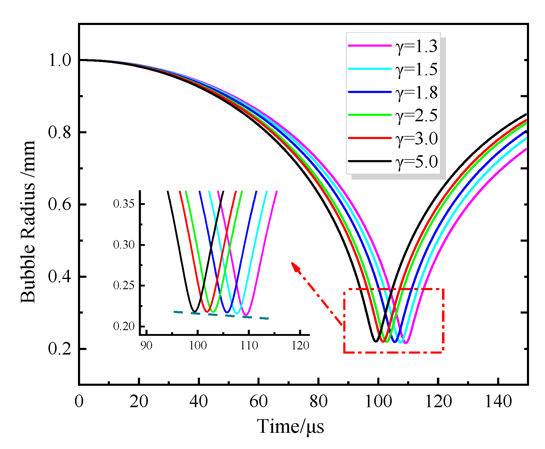
Under near-wall conditions, as the dimensionless distance γ between the bubble and the wall decreases, the time for the bubble to collapse increases, and the minimum radius gradually decreases in a linear fashion.

(2)

The movement of the bubble’s center of mass varies significantly with different values of γ. During the initial stages of collapse, the bubble’s center of mass remains nearly unchanged. However, towards the end of collapse, the bubble’s center of mass rapidly moves towards the wall, with a larger displacement observed for smaller values of γ.

(3)

The peak velocity of bubble translation decreases with increasing γ values, and the peak velocity aligns with the time when the bubble collapses to its minimum radius. For conditions γ = 1.2 and γ = 1.5, the bubble exhibits a phenomenon of moving away from the wall during the rebound phase, with maximum velocities of 22.27 m/s and 7.79 m/s, respectively.

(4)

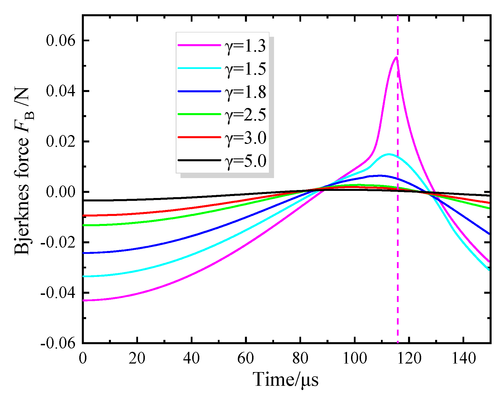
As γ decreases, the secondary Bjerknes force during the initial stage of bubble collapse gradually increases in the form of attraction. Subsequently, during the later stages of collapse and rebound, the secondary Bjerknes force alternates between attraction and repulsion. However, averaging over the entire computational period reveals that bubbles in the near-wall region are primarily subject to attraction, causing them to move towards the wall.

(5)

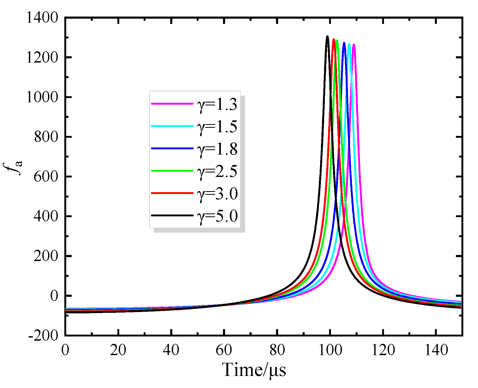
In analyzing the radiated sound pressure at the wall, it was observed that the radiated sound pressure of the bubble decreases in an inverse function trend with the increase in the dimensionless parameter γ. In the case where γ equals 1.3, the radiated sound pressure at the wall is 33.73 times the ambient pressure. Moreover, this paper introduces a radiated sound pressure coefficient to characterize the radial vibration behavior of the bubble. It was found that the distance to the wall has a minor influence on the radiated sound pressure coefficient, providing a basis for future research on bubbles of different scales.

References

1. Fox, F.E.; Herzfeld, K.F. Gas bubbles with organic skin as cavitation nuclei. J. Acoust. Soc. Am. 1954, 26, 984–989. [Google Scholar] [CrossRef]
2. Rayleigh, L. On the pressure developed in a liquid during the collapse of a spherical cavity. Philos. Mag. 1917, 34, 94–98. [Google Scholar] [CrossRef]
3. Plesset, M.S. The dynamics of cavitation bubbles. J. Appl. Mech.-Trans. ASME 1949, 16, 277–282. [Google Scholar] [CrossRef]
4. Gilmore, F.R. The Growth or Collapse of a Spherical Bubble in a Viscous Compression Liquid; California Institute of Technology: Pasadena, CA, USA, 1952; pp. 26–41. [Google Scholar]
5. Keller, J.B.; Miksis, M. Bubble oscillations of large amplitude. J. Acoust. Soc. Am. 1980, 68, 628–633. [Google Scholar] [CrossRef]
6. Sochard, S.; Wilhelm, A.M.; Delmas, H. Modelling of free radicals production in a collapsing gas-vapour bubble. Ultrason. Sonochem. 1997, 4, 77–84. [Google Scholar] [CrossRef] [PubMed]
7. Ida, M.; Naoe, T.; Futakawa, M. Suppression of cavitation inception by gas bubble injection: A numerical study focusing on bubble-bubble interaction. Phys. Review. E Stat. Nonlinear Soft Matter Phys. 2007, 76 Pt 2, 046309. [Google Scholar] [CrossRef] [PubMed]
8. Qinghim; Naranmandula. Influence of large bubbles on cavitation effect of small bubbles in cavitation multi-bubbles. Acta Phys. Sin. 2019, 68, 167–175. [Google Scholar]
9. Best, J.P.; Blake, J.R. An estimate of the Kelvin impulse of a transient cavity. J. Fluid Mech. 1994, 261, 75–93. [Google Scholar] [CrossRef]
10. Li, W.; Li, Z.; Han, W.; Tan, S.; Yan, S.; Wang, D.; Yang, S. Time-mean equation and multi-field coupling numerical method for low-Reynolds-number turbulent flow in ferrofluid. Phys. Fluids 2023, 35, 125145. [Google Scholar] [CrossRef]
11. Li, W.; Li, Z.; Han, W.; Yan, S.; Zhao, Q.; Chen, F. Measured viscosity characteristics of Fe3O4 ferrofluid in magnetic and thermal fields. Phys. Fluids 2023, 35, 012002. [Google Scholar] [CrossRef]
12. Li, W.; Li, Z.; Qin, Z.; Yan, S.; Wang, Z.; Peng, S. Influence of the solution pH on the design of a hydro-mechanical magneto-hydraulic sealing device. Eng. Fail. Anal. 2022, 135, 106091. [Google Scholar] [CrossRef]
13. Ding, Q.; Li, X.; Cui, Y.; Lv, J.; Shan, Y.; Liu, Y. Study on Non-Spherical Deformation Velocity of a Single Cavitation Bubble. Processes 2024, 12, 553. [Google Scholar] [CrossRef]
14. Fourest, T.; Deletombe, E.; Faucher, V.; Arrigoni, M.; Dupas, J.; Laurens, J.M. Comparison of Keller-Miksis model and finite element bubble dynamics simulations in a confined medium. Application to the Hydrodynamic Ram. Eur. J. Mech.-B/Fluids 2018, 68, 66–75. [Google Scholar] [CrossRef]
15. Brennen, C.E. Cavitation and Bubble Dynamics; Oxford University Press: Oxford, UK, 1993. [Google Scholar]
16. Mettin, R.; Akhatov, I.; Parlitz, U.; Ohl, C.D.; Lauterborn, W. Bjerknes forces between small cavitation bubbles in a strong acoustic field. Phys. Rev. E 1997, 56, 2924–2931. [Google Scholar] [CrossRef]
17. Moo, J.G.S.; Mayorga-Martinez, C.C.; Wang, H.; Teo, W.Z.; Tan, B.H.; Luong, T.D.; Gonzalez-Avila, S.R.; Ohl, C.D.; Pumera, M. Bjerknes Forces in Motion: Long-Range Translational Motion and Chiral Directionality Switching in Bubble-Propelled Micromotors via an Ultrasonic Pathway. Adv. Funct. Mater. 2018, 28, 1702618. [Google Scholar] [CrossRef]
18. Cheng, F.; Ji, W. Numerical and experimental study on dynamic characteristics of cavitation bubbles. Ind. Lubr. Tribol. 2018, 70, 1119–1126. [Google Scholar] [CrossRef]
19. Li, F.; Cai, J.; Huai, X.; Liu, B. Interaction Mechanism of Double Bubbles in Hydrodynamic Cavitation. J. Therm. Sci. 2013, 22, 242–249. [Google Scholar] [CrossRef]
20. Faissole, F. Formally-Verified Round-Off Error Analysis of Runge-Kutta Methods. J. Autom. Reason. 2024, 68, 1–33. [Google Scholar] [CrossRef]
21. Devin, C. Survey of Thermal, Radiation, and Viscous Damping of Pulsating Air Bubbles in Water. J. Acoust. Soc. Am. 1959, 31, 1654–1667. [Google Scholar] [CrossRef]
22. Nie, J.-D.; Su, Y.-S.; Yang, G.-M. Numerical Modeling of Noise Generation During Collapse of Single Bubble. Ordnance Ind. Autom. 2009, 28, 23–24. [Google Scholar]
23. Deng, Y.; Jin, T.; Chi, H.; Zhou, J. Collapse of laser induced bubbles and generated sound pressure waves. High Power Laser Part. Beams 2013, 25, 2793–2798. [Google Scholar] [CrossRef]
Figure 1. Diagram of a Bubble Near a Wall.
Processes 12 00826 g001
Figure 2. Variation of Bubble Radius and Bubble Wall Velocity Over Time.
Processes 12 00826 g002
Figure 3. Experimental Setup. (1—High-speed camera (Revealer) with frame rate up to 1 million fps, 2—Water tank (250 mm × 150 mm × 250 mm) and electric discharge device, 3—LED light source, 4—Adjustable DC power supply, 5—Charging and discharging circuit, 6—Computer).
Processes 12 00826 g003
Figure 4. Comparison chart between experiment and simulation.
Processes 12 00826 g004
Figure 5. Grid independence test.
Processes 12 00826 g005
Figure 6. The Bubble velocity field distribution (γ = 1.5).
Processes 12 00826 g006
Figure 7. Evolution process of bubble morphology (γ = 1.5).
Processes 12 00826 g007
Figure 8. Liquid velocity around the bubble(γ = 1.5).
Processes 12 00826 g008
Figure 9. Variation of bubble radius over time under different γ conditions.
Processes 12 00826 g009
Figure 10. Curve of Bubble Center Position Change.
Processes 12 00826 g010
Figure 11. Curve of Bubble Translational Velocity Change.
Processes 12 00826 g011
Figure 12. The change of Bjerknes force over time.
Processes 12 00826 g012
Figure 13. The change of viscous resistance force over time.
Processes 12 00826 g013
Figure 14. Single bubble radiated sound pressure calculation results.
Processes 12 00826 g014
Figure 15. Radiated Sound Pressure Coefficient Variation Over Time.
Processes 12 00826 g015