1. Introduction
China is rich in deepwater oil and gas. According to the results of a resource evaluation by the Ministry of Land and Resources, the current geological reserves of the South China Sea are approximately 23–30 billion tons of oil and 16 trillion cubic meters of natural gas (of which the deepwater area accounts for approximately 70%). This is approximately one-third of China’s total oil and natural gas resources [
1,
2,
3]. China’s dependence on foreign oil continues to remain high, and the eastern part of the South China Sea, as important support for national energy security, will continue to play an important role as the main battlefield for CNOOC’s oil and gas exploration and development. Deepwater oil and gas exploration and development face high risks and uncertainties. Once an overflow or blowout occurs, it can easily cause serious economic losses, platform personnel casualties, and pollution of the marine environment. Finding the shut-in pressure of oil and gas wells quickly and accurately in the case of overflow is crucial to ensure the safe and efficient production of typical “double-deep and double-high wells” in the eastern part of the South China Sea.
Some indoor experiments and theoretical modeling have been carried out by researchers to study such problems. Leblanc and Lewis [
4] established the first wellbore pressure prediction model for the drilling process after gas intrusion, which is a homogeneous flow model that does not take into account inter-phase interactions or annulus friction pressure depletion. Nunes [
5] proposed a multiphase flow model for deepwater and ultra-deepwater straight well drilling, assuming that the bottomhole pressure during drilling gas intrusion stays constant. A multiphase flow model applicable to deepwater and ultra-deepwater straight well drilling was developed, and the pressure distribution in the annulus and throttling line and the cross-sectional gas content rate distribution were obtained. The model comprehensively considered factors such as water-based drilling fluid, well structure, and working conditions, such as gas intrusion and pressure well. Its limitation is that the pressure calculation of the gas-liquid two-phase flow in the wellbore was established based on the segmented plug flow pattern, which is applicable to the conditions of atmospheric intrusion. Meipeng [
6] established a model of gas slippage during well shut-in and a calculation model of wellbore pressure considering the combined effects of wellbore renewal and gas slippage during well shut-in and gave a method for reading wellbore pressure of gas intrusion shut-in wells based on this model. Shihui et al. [
7] developed a computational model to predict bottomhole and wellhead pressures during well shut-in, incorporating the wellbore storage effect. The analysis revealed the dynamics of bubble transport along the wellbore under simulated shut-in conditions. They highlighted the risks associated with prolonged shut-ins following gas intrusion, emphasizing the potential for exceeding maximum shut-in jacket pressure. To mitigate this risk, they recommended employing throttle valves to release sprays and pressure. This approach allows for conditional gas expansion and rapid re-pressurization and venting of the well to reestablish pressure equilibrium. Abdelhafiz [
8] established a numerical model for the temperature distribution of the vertical drilling system under circulating and shut-in conditions, which simulated the temperature distribution of the drilling fluid, the drilling column, casing column, the back of the casing cement, and the transient temperature perturbation of the surrounding rock formation. The curves obtained from the simulation are in agreement with the results of FLUENT software. For more information on FLUENT, visit the ANSYS official website at [
www.ansys.com] (
https://www.ansys.com).
Li [
9] simulated the dynamic change in wellbore pressure after overflow shutdown by solving the multiphase flow model of a gas wellbore after overflow shutdown and realized the dynamic simulation of overflow shutdown and real-time calculation of wellbore pressure. They were able to accurately obtain the formation pressure and describe the information of the wellbore and formation using the relationship between the shutdown time and the recovery of bottomhole pressure. Xinyue [
10] found that a nonstationary heat transfer model considering the wellbore temperature during well shut-in can correct the abnormal pressure recovery curve during well shut-in and make the test well interpretation results closer to the measured values. Yu [
11] quantitatively described the loss of kinetic energy of the gas flow, water strike wave transfer velocity, and friction loss in the water strike effect during quick shut-in recovery at the wellhead of a high-temperature and high-pressure gas well by establishing a single-phase gas wave velocity model based on the control equation of the wellbore pressure–temperature coupling calculation. Baojiang and Zhiyuan et al. [
12] established a transient wellbore multiphase flow model considering the interphase mass and heat transfer laws under different flow conditions and the mutual coupling between the wellbore and formation, which can accurately predict the multiphase flow pressure in the wellbore. Chaodong et al. [
13] established a model of the wellbore multiphase water strike pressure triggered by the gas intrusion shut-in of deep wells and investigated the influence of parameters such as shut-in time, well depth, and gas intrusion volume on the wellbore multiphase water strike pressure in the process of well shut-in. Gou [
14] summarized the commonly used single-phase flow and multiphase flow pressure-drop calculation models, preferred the corresponding pressure calculation method through comparative analysis, coupled the unsteady-state temperature model with the pressure model and iterative calculation, and analyzed the factors influencing the temperature and pressure distribution of the wellbore in the process of well startup and shutdown for reference in the dynamic analysis of high-temperature and high-pressure gas wells.
Based on the principle of gas-liquid two-phase flow, Pu [
15] established physical and mathematical models of the initial state of the wellbore annulus under overflow conditions and proposed an inversion method for solving the mathematical model, which addressed the difficult problem of calculating the initial state of the wellbore annulus after well shutdown by overflow. Chen [
16] considered a calculation method for wellbore heat transfer, temperature, and pressure coupling applicable to steady flow, deduced from the basic equations, and established a temperature-pressure coupling calculation model considering wellbore renewed flow and heat transfer between the wellbore and the surrounding strata or seawater. They successfully applied it to the calculation of the bottomhole restoration pressure of the shut-in M1 gas field in the Western South China Sea offshore wells and the analysis of the test wells. However, the model is not applicable to transient flow during the well shut-in period. Bing [
17] studied the yield stress and shear dilatancy characteristics of drilling fluids with non-Newtonian fluids. Analyzing the influence of the gas distribution coefficient on wellbore pressure calculations provides a theoretical basis for the calculation of wellbore pressure in shut-in wells. Xin et al. [
18] established a transient flow model of a gas-liquid two-phase flow in a wellbore based on the drift model for complex multiphase flow in the wellbore and solved it using the AUSMV format with high computational accuracy. Using MATLAB software, the gas-liquid two-phase flow law in a wellbore under gas intrusion was programed and simulated, which can serve as a theoretical guide for the accurate calculation of the relevant pressure parameters after well shut-in. For more information on MATLAB, visit the MathWorks official website at [
www.mathworks.com] (
https://www.mathworks.com).
The wellbore expansion and the thermal expansion of the fluid caused by the wellbore temperature field have a large impact on shut-in pressure, which has not been fully considered in previous studies. Therefore, this study comprehensively considers the pressure solution for the shut-in of a typical “double-deep and double-high” oil and gas well in the South China Sea under the conditions of heat-fluid-solid coupling.
2. Materials and Methods
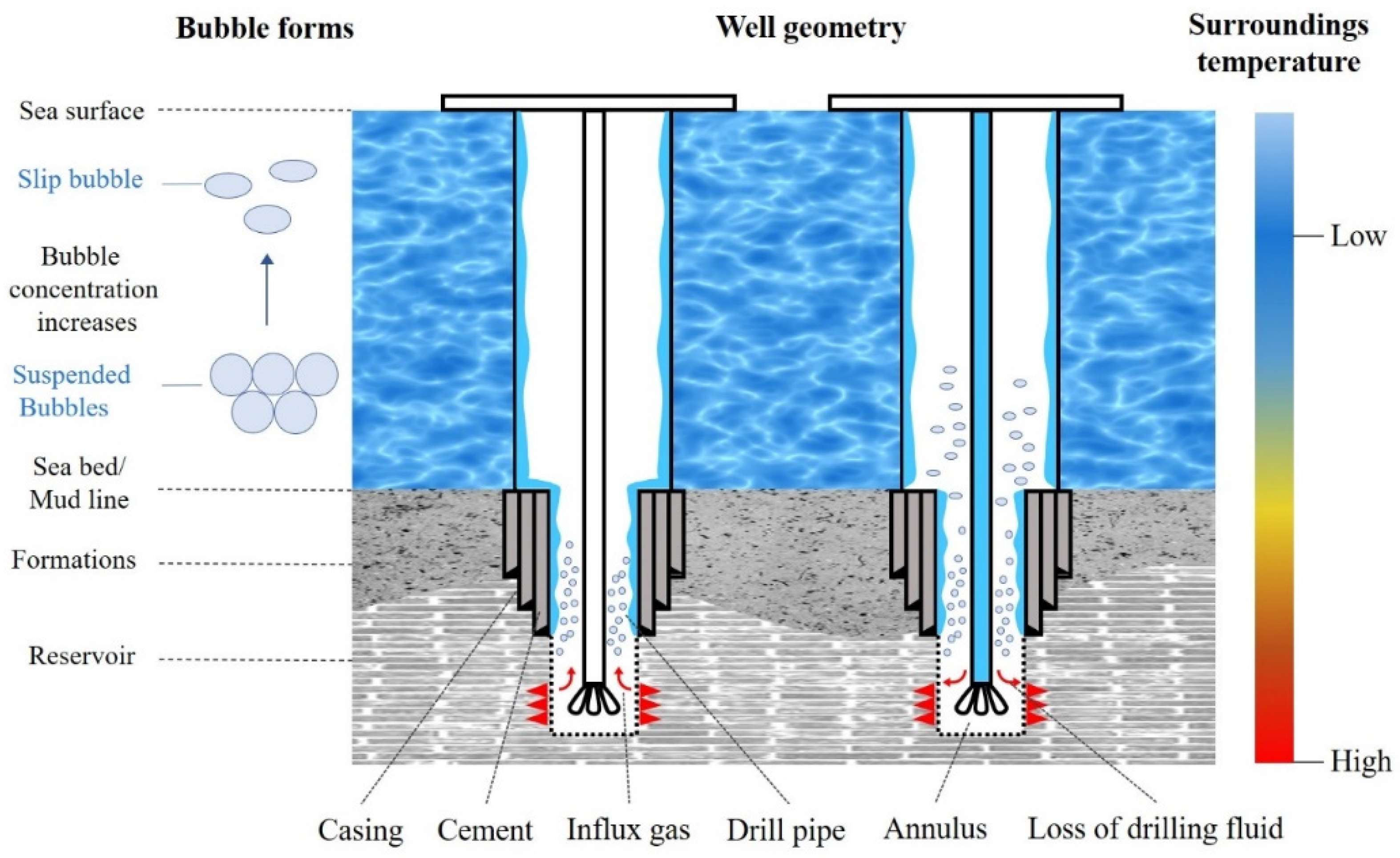
As shown in
Figure 1, when well control problems, such as blowout or sudden large amounts of gas entering the drilling fluid system, are encountered during deepwater drilling, it is necessary to take measures to shut down the well to prevent blowout accidents from occurring. The shutdown process is more complicated compared to land because of the high-pressure and low-temperature environmental conditions of the seafloor in deepwater drilling, which involves the change mechanism of the multi-field coupling of the heat-flow curing and mainly includes the following aspects:
(1) The drilling fluid is typically a non-Newtonian fluid. After the gas intrusion shut-in is affected by the fluid yield stress and other factors, the gas exists in the form of a suspension in the drilling fluid until it exceeds the limiting suspension concentration of the gas, after which the gas continues to slip and rise in the wellbore.
(2) A complex coupled flow exists between the wellbore and the formation. In the process of well shut-in, the bottomhole pressure gradually recovers, and under the influence of the pressure difference between the bottomhole and the formation, the formation fluid continues to intrude into the wellbore, but the rate of intrusion varies with time. When the bottomhole pressure exceeds the formation pressure, the drilling fluid in the well leaks into the formation. The coupled flow state between the wellbore and formation has an important effect on the wellbore flow and pressure changes after well shut-in.
(3) After the well is shut in, the fluid temperature in the wellbore gradually changes under the influence of the coupled wellbore formation heat transfer, which affects the compression and expansion of the fluid.
2.1. Shut-In Wellbore Gas Transport and Pressure Prediction Model
The multiphase flow state in the wellbore after shut-in is mainly affected by gas suspension transport in the wellbore and the coupled wellbore–reservoir flow. Thus, a model is established to predict gas transport and pressure in the wellbore after shut-in.
2.1.1. Gas Transport Model in Wellbore
Gas transportation in a wellbore is divided into two main states: suspension and slip-up. When the gas concentration in the cross-section of the wellbore is lower than the limiting suspension concentration, the gas transportation velocity is zero. When the limiting suspension concentration is exceeded, the gas bubbles slip off and rise under the effect of buoyancy.
Gas Suspension Concentration Prediction Model
Gas suspension is affected by the bubble’s own buoyancy, fluid yield stress, surface tension, and shear dilatancy, and the limiting suspension concentration is generally obtained based on the gas limiting suspension test, which is represented by the empirical model [
19] as:
where
Bi is the critical levitation condition reached by a single bubble (dimensionless),
τy is the yield stress of the fluid (Pa),
ρl is the density of the liquid (kg/m
3),
ρg is the density of the gas (kg/m
3),
g is the acceleration of gravity (m/s
2)
, and
Reff is the equivalent radius of the bubble (m).
where
EF is the limiting suspended volume fraction of gas without factorization.
Gas Transport Velocity Prediction Model
When the total volume of the wellbore annulus is certain after the well is shut in, the drilling fluid rheology and size of the gas bubbles have an important effect on the rate of sliding rise of the gas in the wellbore, where the average equivalent radius of the gas bubbles can be expressed by empirical equations under the effect of differential pressure:
where
is the mean equivalent radius (m), and
φp is the formation porosity without factorization.
Starting from the bottom of the well, when the gas volume in the well section reaches the limiting suspended volume fraction, the remaining gas slips off and rises. Shaowei [
20] found that the Margaritis model [
21] can be used for the bubble transport velocity in yield stress fluids at Re < 20 or Re > 50, and Rodrigue’s small Reynolds number method [
22] is more applicable at 20 < Re < 50, where the drag force coefficient is corrected:
where
CD is the drag force coefficient without factorization,
ub is the bubble slip velocity (m/s), and
Re is the Reynolds number.
Based on the above equation, and then combined with the definition of the drag force coefficient, we establish an expression for the bubble rise velocity as:
where
Vb is the bubble volume (m
3).
2.1.2. Wellbore–Stratigraphic Couple
Two working conditions, formation gas intrusion and wellbore-drilling-fluid filtration loss, occur between the wellbore and formation owing to the pressure difference, where the gas intrusion volume can be expressed as follows when the bottomhole pressure is less than the formation pressure:
where
Qg(
t) is the gas intrusion velocity under standard condition (m
3/s),
pp is the formation pressure (Pa),
pw(
t) is the bottomhole pressure at time t (Pa),
μg is the gas viscosity (Pa
−s),
Z is the gas compression factor under the wellbore temperature-pressure condition,
Pa is the standard atmospheric pressure (Pa),
T is the wellbore temperature (K),
re is the effective radius of the reservoir (m),
k is the formation permeability (m
2),
h is the height of the seepage well section (m),
Za is the gas compression factor under the standard temperature-pressure condition,
Ta is the standard temperature (K),
rw is the radius of the well borehole (m), and
ρga is the density of gas under standard condition (kg/m
3).
As the gas intrudes and rises into the wellbore, the pressure in the wellbore gradually increases. Once the pressure at the bottom of the well exceeds the formation pressure, the drilling fluid begins to leach into the formation. When the viscosity of the drilling fluid is significantly greater than that of the reservoir fluid, the amount of leaching is determined primarily by the viscosity of the fracturing fluid. The Darcy equation can be used to calculate the filtration loss coefficient
C1 controlled by the viscosity of the drilling fluid as:
where
C1 is the filtration loss coefficient controlled by the viscosity of the fracturing fluid (m·min
−0.5), and
μm is the viscosity of the drilling fluid (mPa·s).
When the viscosity of the drilling fluid is close to that of the reservoir fluid, filtration loss is mainly determined by the compressibility of the formation rock and fluid. According to Darcy’s percolation equation, the filtration loss coefficient
C2 is governed by the compressibility of the formation rock and fluid.
where
Cf is the integrated compression coefficient of the formation fluid (MPa
−1).
In addition, the filtration loss coefficient
C3 of the wall-forming fracturing fluid was obtained by testing.
where
C3′ is the loss coefficient obtained from the test (m·min
−0.5),
C3 is the loss coefficient under the bottomhole differential pressure (m·min
−0.5), and Δ
p′ is the test differential pressure (Pa).
The combined loss coefficients and drilling fluid filtration rates in the actual drilling process are obtained from the partial pressure drop equation by considering the three cases together.
where
Ql is the filtration rate of the drilling fluid (m
3/s) and
t0 is the moment when the bottomhole pressure is greater than the formation pressure.
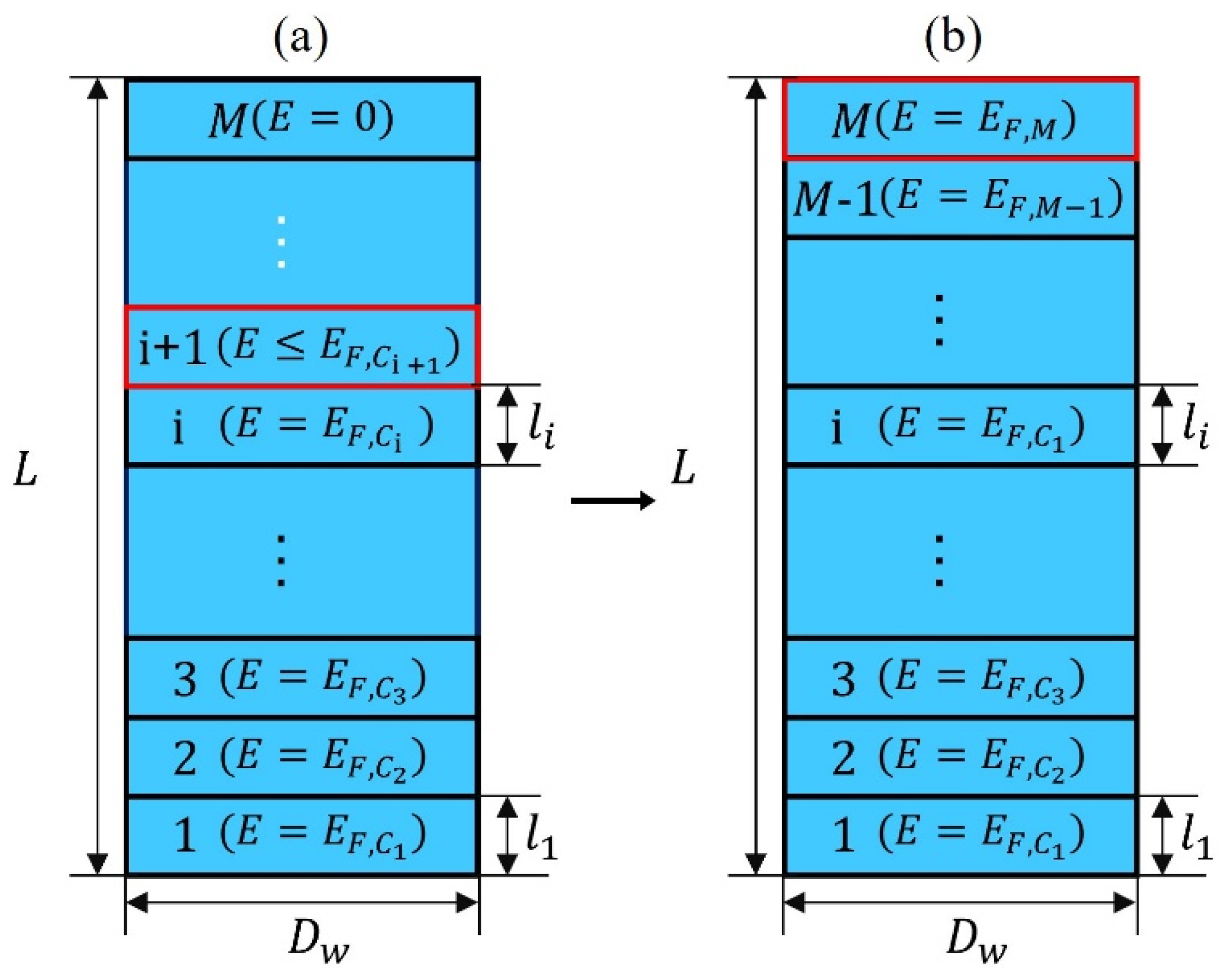
2.1.3. Wellbore Pressure Calculation
To simulate the variation in pressure in the well after the shut-in, the wellbore is divided into M segments, as shown in
Figure 2, where E is the gas content. The gas rises from the bottom of the well, and the rise stops when the gas content reaches a certain limit in each segment. When the initial gas intrusion is small, the gas is completely suspended in the well section, as shown in
Figure 2a. When the gas intrusion is large, a high-pressure gas compartment may form at the wellhead, as shown in
Figure 2b.
The total volume of gas intruding into the wellbore at the time of shut-in is
V0, and the initial wellhead pressure is 0. The initial bottomhole pressure is expressed as:
where,
pw0 is the bottomhole pressure at the initial moment (Pa),
ρm is the density of drilling fluid (kg·m
−3),
L is the depth from the wellhead to the bottomhole (m), and
A0 is the cross-sectional area of the annulus at the bottomhole (m
2).
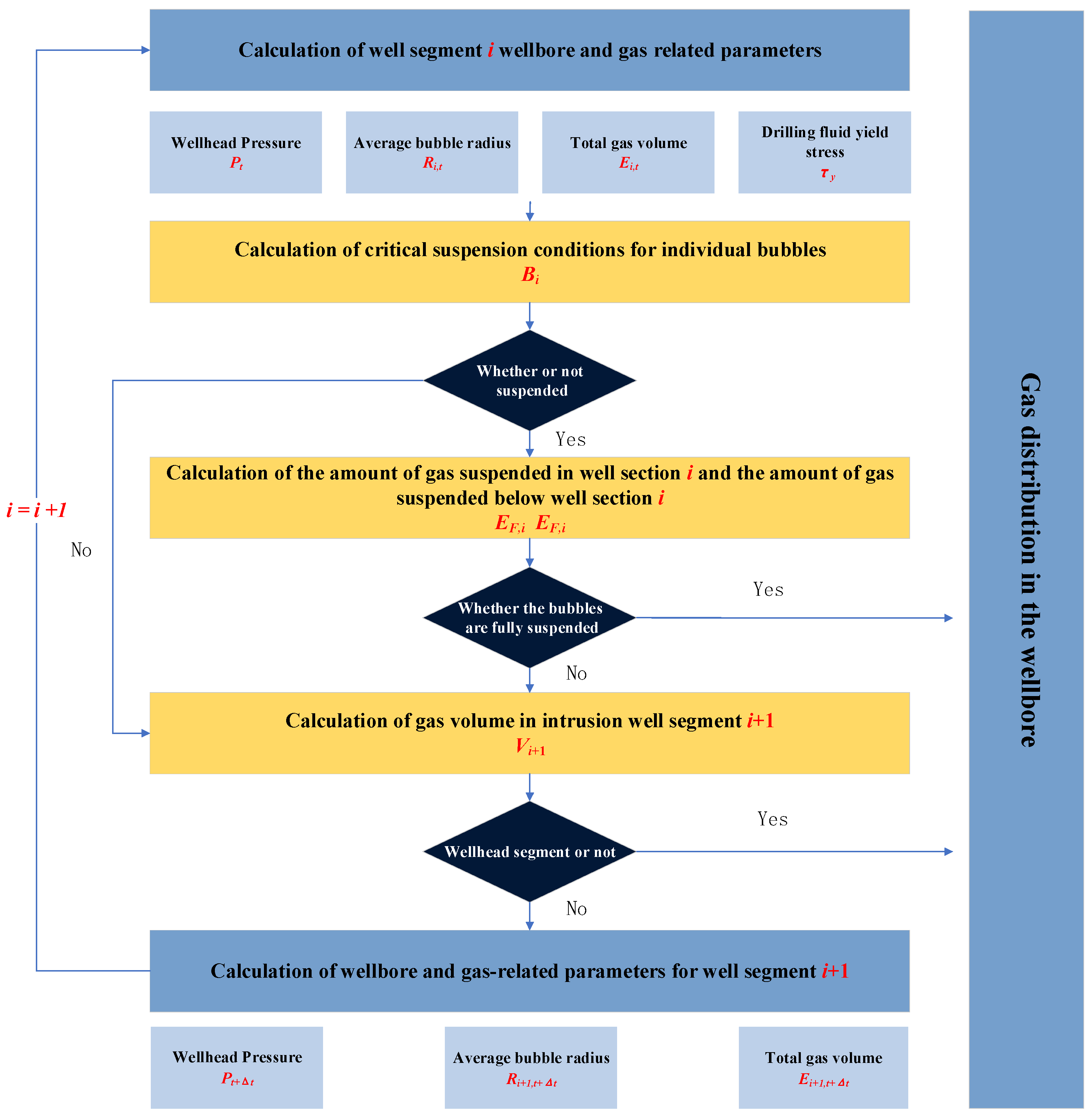
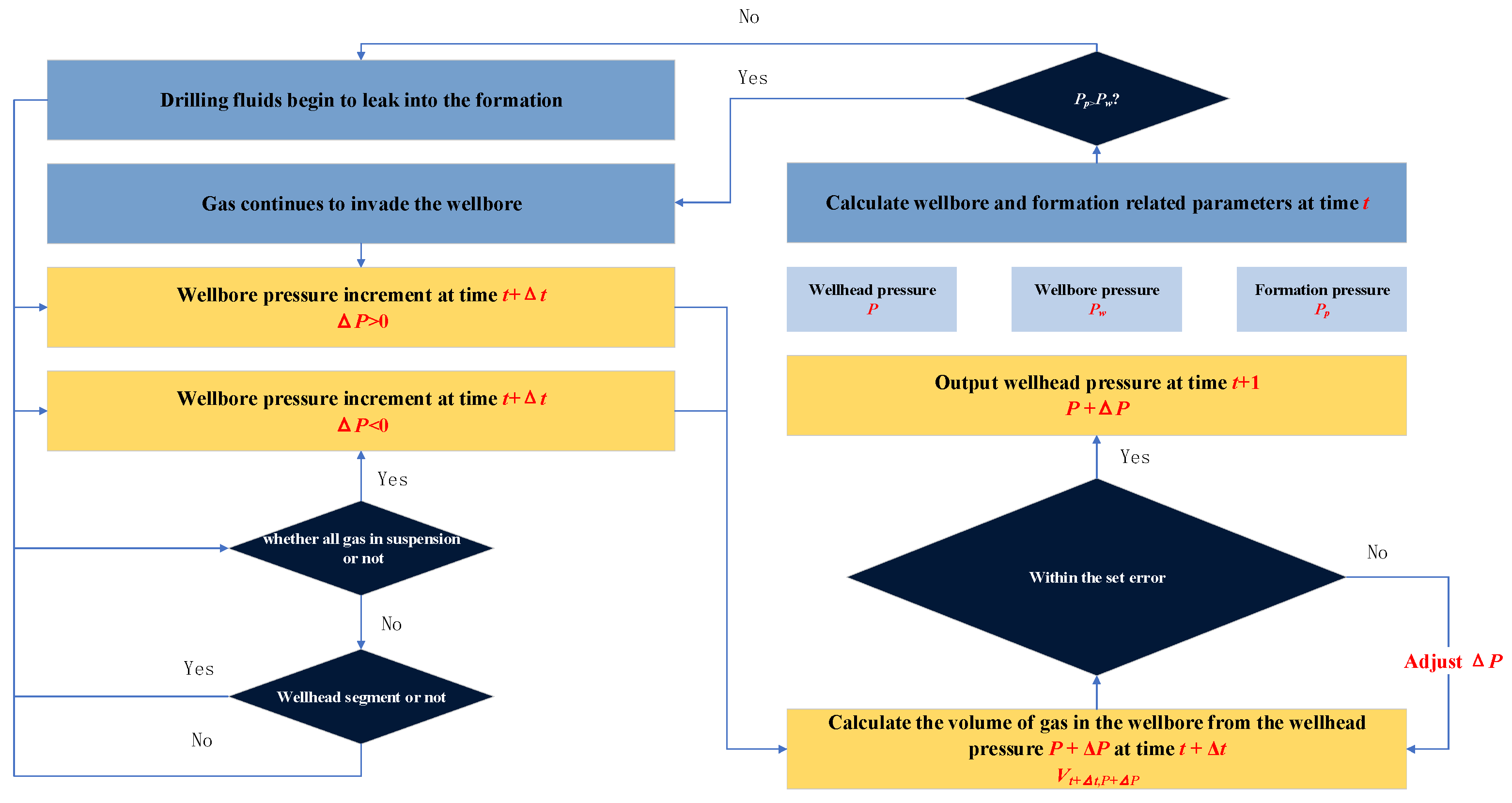
As the gas rises in the wellbore, its transport and suspension states can be quantified by calculating the position of the leading edge of the gas using Equations (3)–(6) to determine the suspended volume fraction of the gas. As the gas is transported upward, the pressure in the wellbore increases, which affects the volume of the bubbles and the suspended volume fraction. To accurately calculate the change in pressure in the wellbore, the model is determined numerically in this study using the finite difference method, which involves calculating the distribution of the gas in the wellbore and the pressure at the wellhead. The solution process is as follows (
Figure 3):
The wellbore pressure solution process is shown in
Figure 4.
The interval time step Δ
t denoted in the above figure is:
where
ub(i,t) is the gas rise velocity in cell
i at time
t (m/s).
Neglecting the wellbore elasticity and drilling fluid compressibility, the amount of suspended gas in cell
i is obtained from the gas equation of state as follows:
where
ng is the amount of gas substance (mol),
Vi is the total volume of transported gas in the
ith cell (m
3),
Zi is the gas compression factor at the bottom of the well and the
ith cell (dimensionless),
Ti is the temperature at the bottom of the well and the
ith cell (°C),
hi,
hk are the heights of the
ith and the
kth cell, respectively (m), and
pCi is the pressure at the mouth of the well when the gas rises to the
ith cell (Pa).
The value of
EF,i is
EF,Ci when a single bubble in the
ith cell can remain suspended, and the value of
EF,i is 0 when a single bubble cannot remain suspended. The total amount of substance of all suspended gases is:
The volume of gas, single bubble volume into the (
i + 1)th cell, is:
When the bubble rises to the (
i + 1)th cell, the pressure at the wellhead is
pCi+1. Neglecting the change in the compression factor caused by the change in the pressure at the wellhead from
pCi to
pCi+1, the volume of a single suspended bubble in the
kth (
k <
i) cell becomes:
where
ρmj,i is the actual density of drilling fluid in the
jth cell when the gas rises to the
ith cell (kg/m
3),
ρgj,i is the actual density of gas in the
jth cell when the gas rises to the
ith cell, which can be calculated by the gas equation of state (kg/m
3), and
EF,Cj,i is the limiting suspension of the gas in the
jth cell when the gas rises to the
ith cell (dimensionless).
2.2. Wellbore Temperature Field Models after Well Shut-In
In the above equation, the change in temperature has a large impact on the fluid density, which in turn affects the calculation of the wellbore pressure after shut-in; thus, modeling the temperature field around the wellbore after shut-in is the basis for wellbore pressure after gas intrusion shut-in. According to the principle of energy conservation of the unit control components (inside the drilling column, wall of the drilling column, annulus, casing, cement ring, and formation), a one-dimensional fluid in the wellbore and a two-dimensional transient mathematical model of the formation are established.
2.2.1. Temperature Field Equations
The temperature variation of the fluid in the wellbore is mainly subject to the processes of heat transfer within the drill column from the drill column wall, in the annulus, and near the well wall, which are modeled separately below.
Heat Transfer within the Drilling Column Model
The heat exchange within the drilling column mainly considers the convective heat transfer between the drilling fluid and the drilling tool wall in the upward direction. The mathematical model can be expressed as follows:
where
λm is the thermal conductivity of drilling fluid (W/(m·°C)),
λw is the thermal conductivity of the wall of the drilling column (W/(m·°C)),
Tw is the temperature of the wall of the drilling column (°C), Tc is the temperature inside the drilling column (°C),
r0 is the inner radius of the drilling column (m),
r1 is the outer radius of the drilling column (m),
cm is the specific heat capacity of the drilling fluid (J/(K·kg)), and
ρm is the density of the drilling fluid (kg/m
3).
Drilling Column Wall Heat Transfer Model
The model mainly considers heat exchange via convective heat transfer with the drilling fluid in the drilling column and the annulus in the warp direction, which can be expressed as follows:
where
λ3 is the thermal conductivity of well wall medium (W/(m·°C)), and
r2 is the radius of the annulus (m).
Annulus Heat Transfer Model
The main factor affecting the annulus heat transfer model is the heat generated by convective heat transfer with the well wall and outer wall of the drilling column in the radial direction, which can be expressed as follows:
where
Ta is the temperature of the annulus (°C), and
r3 is the wall radius (m).
Near-Well Wall Heat Transfer Model
The well wall avoidance temperature distribution is primarily affected by the heat conduction generated by the cement ring in the radial direction and the convective heat transfer generated by the drilling fluid in the annulus. It can be expressed mathematically as follows:
where
T is the temperature (°C),
ρx is the density (kg/m
3),
cx is the specific heat capacity (J/(kg·°C)),
rx is the radius (m),
λx is the thermal conductivity (W/(m·°C)), where 3 ≤
x ≤ 11, and
x = 3 is the heat transfer medium of the well wall,
x = 4 is the cement ring,
x = 5 is the casing and the cement ring,
x = 6 is the casing and the cement ring, and
x > 7 is the ground layer.
2.2.2. Initial and Boundary Conditions during Well Shut-In
(1) The initial temperature of the drilling fluid in the drill pipe, the drill pipe wall, the drilling fluid in the annulus, the casing, the cement ring, and the formation is the downhole temperature at the end of the cycle.
(2) The surface of the well wall flows out of the formation and transfers equal amounts of heat to the annulus.
(3) The temperature of the formation outflow away from the borehole is the original formation temperature, and the surface is adiabatic in the atmosphere.
3. Results
3.1. Shut-In Well Pressure Model Validation
The well shut-in pressure model developed in this study, considering heat-fluid-solid coupling, was validated using the field data of the well BY5-2-1 well surge shut-in. The well was straight, with a water depth of 816.5 m and a design depth of 4430 m. At 03:18, the 8-1/2-inch borehole was drilled to 4370.7 m, the mechanical drilling speed rose rapidly from 6.69 m/h to 25.6 m/h, and the big hook suspended weight suddenly increased. At 04:20, the well was drilled to 4383.31 m, the EKD return flow rate increased, the wellhead exhibited a gas return, and the full volume of the gas rose rapidly to more than 50%. At 50%, the mud-pool increment was 4 bbl when the well was shut in quickly, and the casing pressure was 500 psi after 33 min of shut-in. The basic parameters of the well are listed in
Table 1.
The structure of the well was as follows: 20” casing × 70 m + 17 -1/2” casing × 900 m + φ311 mm bare hole × 4383.31 m. The combination of drilling tools used was mainly as follows: EH1317 φ319 mm PDC × 0.41 m + φ216 screw × 8.66 m + 9” non-magnetic drill collars × 1 pc + 9” collars × 3 pcs + 8” collars × 5 pcs + drilling percussion × 7.27 m + 5” collars × 7.27 m. 7.27 m + 5” weighted drill pipe × 120.53 m + 5” drill pipe × 1392.56 m + 5 -1/2” drill pipe.
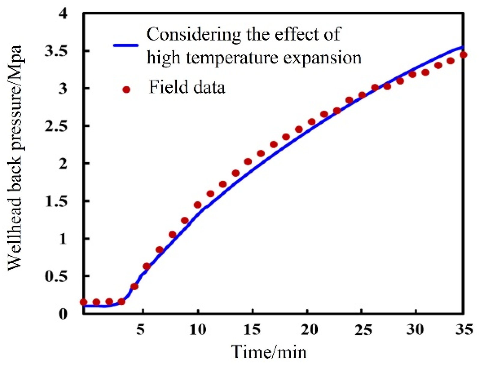
The overflow shut-in process of the well was simulated by applying the established shut-in pressure model considering heat–fluid–solid coupling. The comparison between the calculated and measured values of the shut-in jacket pressure is shown in
Figure 5.
After 33 min of shutting down the well, the measured casing pressure was 3.45 MPa and the casing pressure calculated by the model was 3.55 MPa, indicating an error of 2.89%. The average error in the casing pressure increase was 5.42% during the entire well shut-in process. Therefore, the well shut-in pressure model established in this study has high accuracy and can be applied in engineering practice.
3.2. Analysis of Transient Well Shut-In Processes
The previous analysis showed that the temperature of the wellbore changes during the shut-in process. This happened owing to the natural convective heat transfer in the drill pipe and forced convective heat transfer in the annulus, which in turn caused a change in the physical properties of the two-phase fluids in the annulus of the wellbore, thus affecting the calculation of the shut-in pressure.
3.2.1. Wellbore Temperature
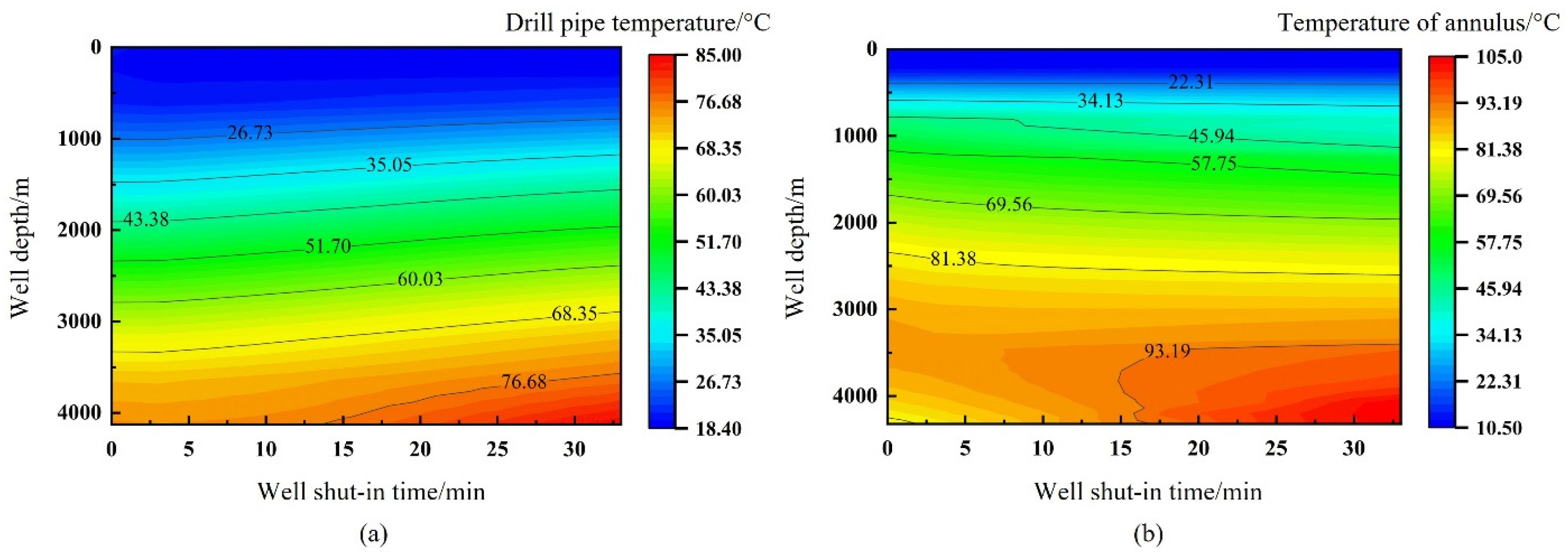
Two-dimensional cloud plots of the changes in the drill pipe and annulus temperatures with shut-in time during the shut-in process are shown in
Figure 6a,b, respectively. The drill pipe and annulus temperatures near the bottom of the well increased gradually with the well shut-in time. After 33 min of well shut-in, the temperature at the bottom of the well increased from 79.9 to 104.4 °C, and the temperature at the annulus mudline decreased from 47.77 to 39.74 °C. After the well was shut in, the temperature near the bottom of the well increased, leading to fluid expansion, and the temperature in the other well sections decreased, leading to fluid contraction. However, from the above temperature changes, it can be seen that the expansion effect due to warming was greater than the contraction effect due to temperature reduction.
3.2.2. Fluid Thermal Expansion
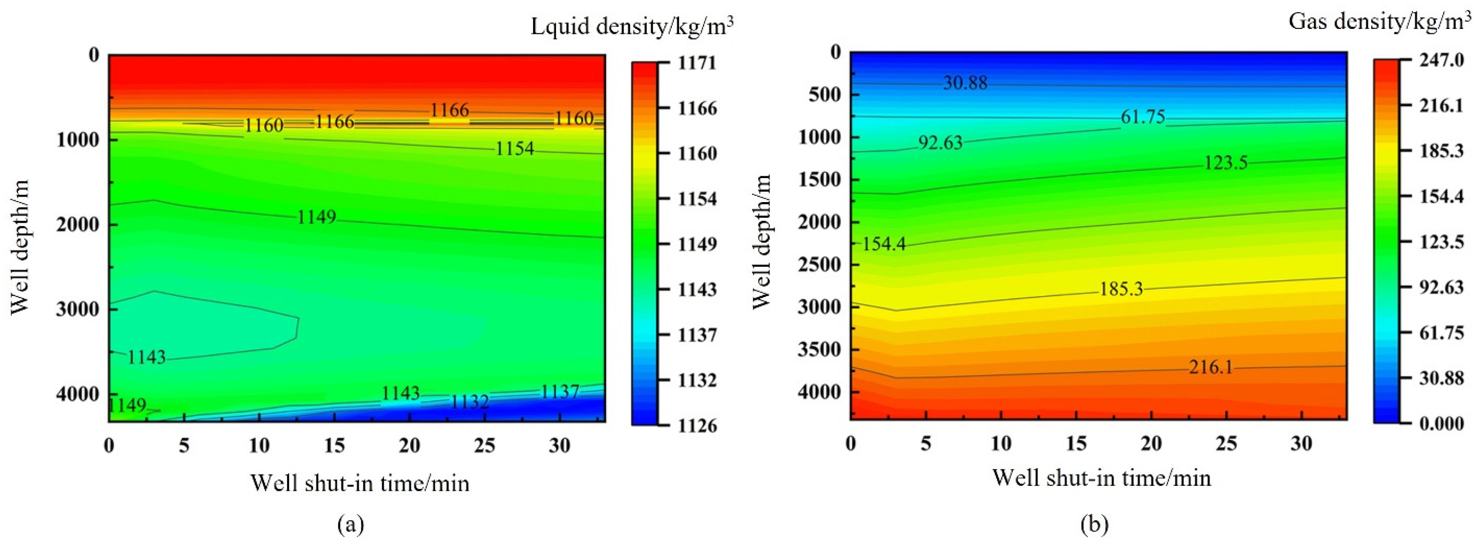
Two-dimensional cloud plots of fluid density and gas density variations with shut-in time during well shut-in are shown in
Figure 7a,b, respectively. The density of the fluids (drilling fluid and gas) near the bottom of the well gradually decreased with the well shut-in time owing to the influence of the wellbore temperature. After 33 min of well shut-in, the density of drilling fluid at the bottom of the well decreased from 1152.9 to 1132.2 kg/m
3 and the density of gas decreased from 246.5 to 232.7 kg/m
3. The effect of warming was greater than that of cooling, and the change in the thermal expansivity of the fluids in the closed wellbore influenced the process of increasing the shut-in jacket pressure.
3.2.3. Wellbore Pressure
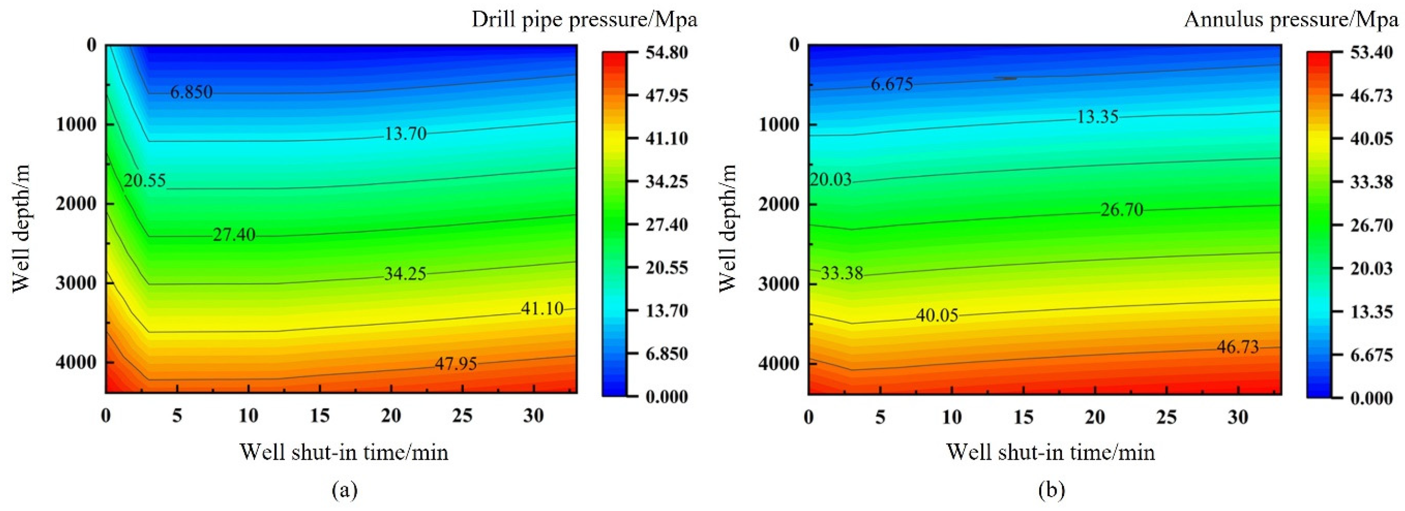
Two-dimensional cloud plots of the changes in the drill pipe pressure and annulus pressure with shut-in time during the well shut-in process are shown in
Figure 8a,b, respectively. The drill pipe and annulus pressure profiles gradually increased with well shut-in time, owing to the wellbore temperature and fluid thermal expansivity. After 33 min of well shut-in, the casing pressure increased from 0.1 to 3.55 MPa, and the bottomhole pressure increased from 52.19 to 53.30 MPa. Owing to the effects of fluid and wellbore thermal expansivity, the increase in wellhead pressure was greater than the increase in bottomhole pressure. Focusing on the analysis of the wellbore temperature field change during the shut-in period, the thermal expansion of the fluid and wellbore affected the recovery of the wellhead pressure during the shut-in period.
3.3. Sensitivity Analysis of Shut-In Wells for Pressure
From the temperature field calculations, the wellbore temperatures gradually increased to the ground temperature gradient during well shut-in. Therefore, the ground temperature gradient mainly affected the wellbore temperature distribution before shut-in and the rise of the wellbore temperature after shut-in. Influenced by the wellbore temperature, the physical properties of the fluid changed, affecting the wellbore pressure.
3.3.1. Analysis of Well Closure under Different Geothermal Gradients
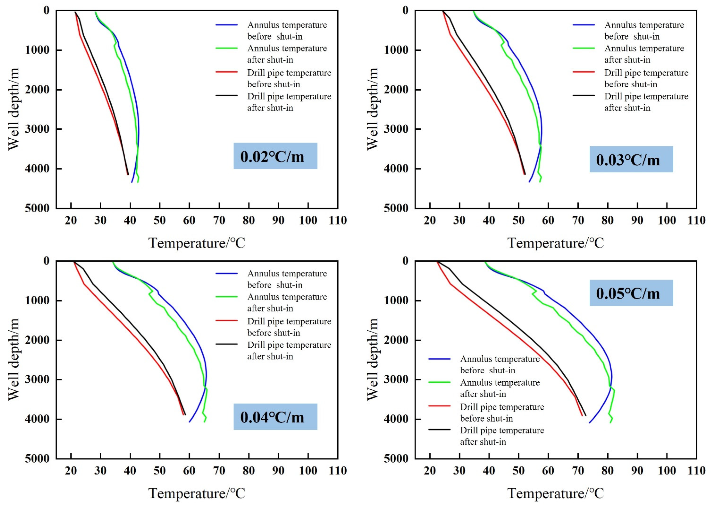
Wellbore Temperature and Fluid Thermal Expansion
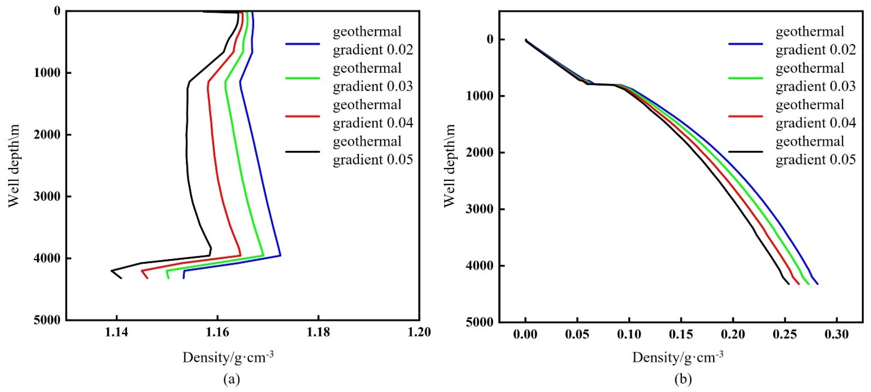
Figure 9 shows the temperature changes in the wellbore before and after well closure under different ground temperature gradients. The larger the ground temperature gradient, the faster the increase in temperature of the wellbore after well shut-in, owing to the influence of heat transfer between the annulus and the formation, and the more evident the influence of the fluid’s physical properties.
Figure 10a,b show the liquid and gas densities, respectively, at the end of well shut-in. The larger the ground temperature gradient, the more evident the effect of thermal expansion and the smaller the gas–liquid density. When the ground temperature gradient increased from 0.02 to 0.05 °C/m, the liquid density at the bottom of the well decreased from 1153 to 1141 kg/m
3 and the gas density decreased from 282 to 254 kg/m
3.
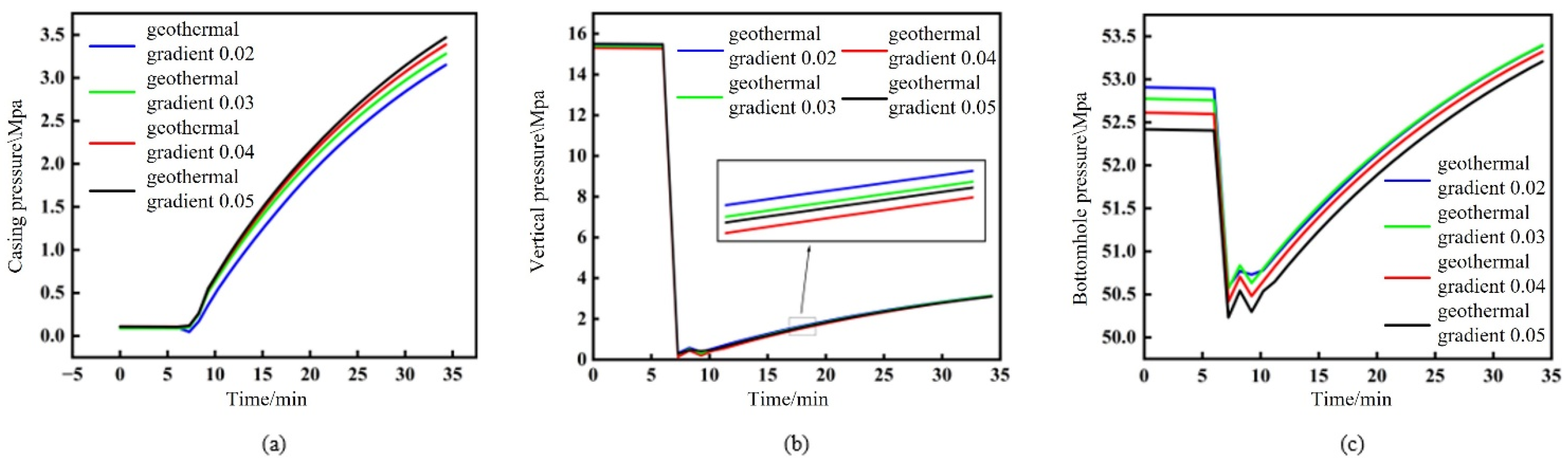
Wellbore Pressure after Shut-In
Figure 11a–c show the changes in the shut-in jacket pressure, shut-in stand pressure, and wellbore pressure, respectively, with shut-in time for different geothermal gradients. For the same well shut-in time, the larger the ground temperature gradient, the smaller the fluid density, resulting in a smaller bottomhole pressure and a larger wellhead pressure. When the ground temperature gradient increased from 0.02 to 0.05 °C/m, the casing pressure changed from 3.15 to 3.47 MPa after the same time of well shut-in.
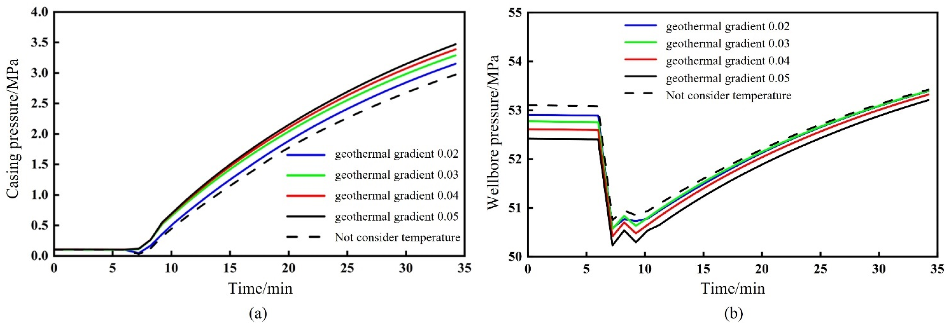
Effect of Fluid Thermal Expansion on Shut-In Well Pressure Seeking
Figure 12a,b show the effects of thermal expansion, being considered or skipped, on the shut-in jacket pressure and bottomhole pressure calculations for different ground temperature gradients. The figures show that the fluid density decreased after considering the thermal expansion of the fluid, compared to when not considering the thermal expansion of the fluid. The wellbore backpressure was higher after shutting off the well at the same time.
3.3.2. Well Shut-In Pressure Analysis with Different Mud Pool Increments
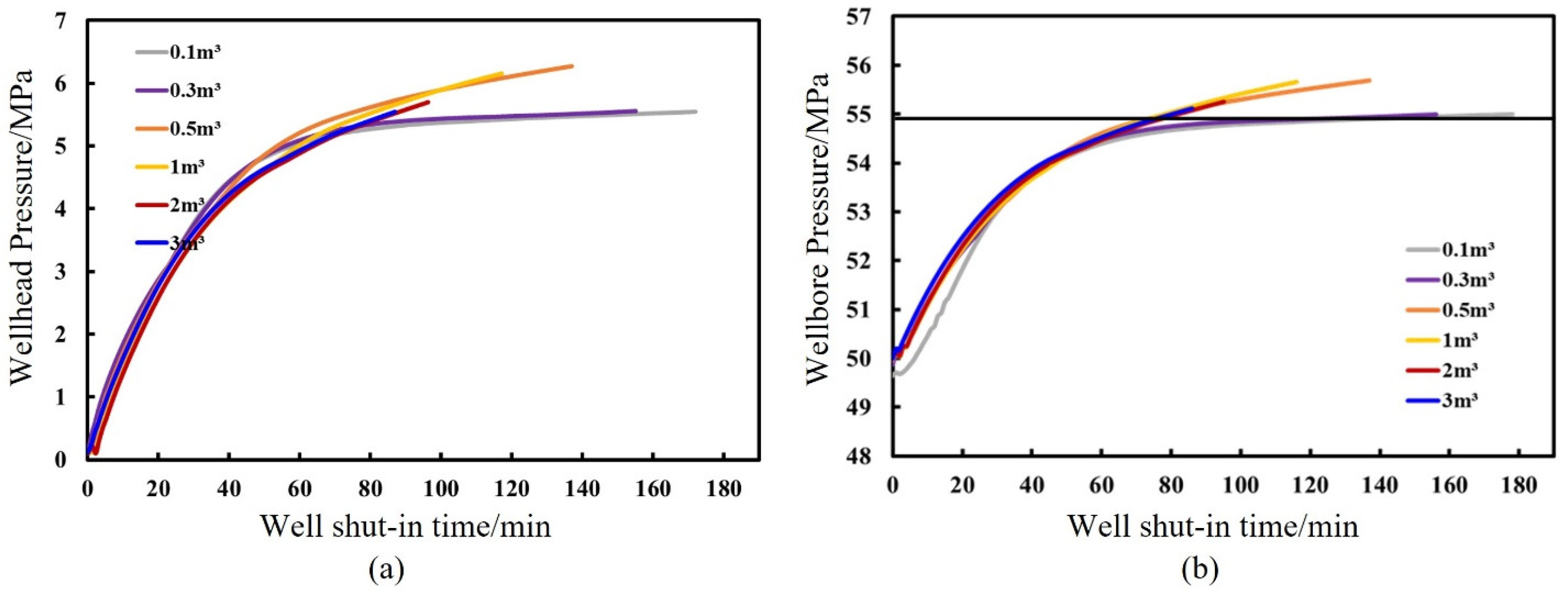
Figure 13a,b shows the variation in the shut-in jacket pressure and wellbore pressure with shut-in time under different mud-pool increment shut-in conditions. The larger the mud-pool increment before well shut-in, the greater the gas intrusion and the faster the gas slip rises, resulting in a faster recovery of wellbore pressure.
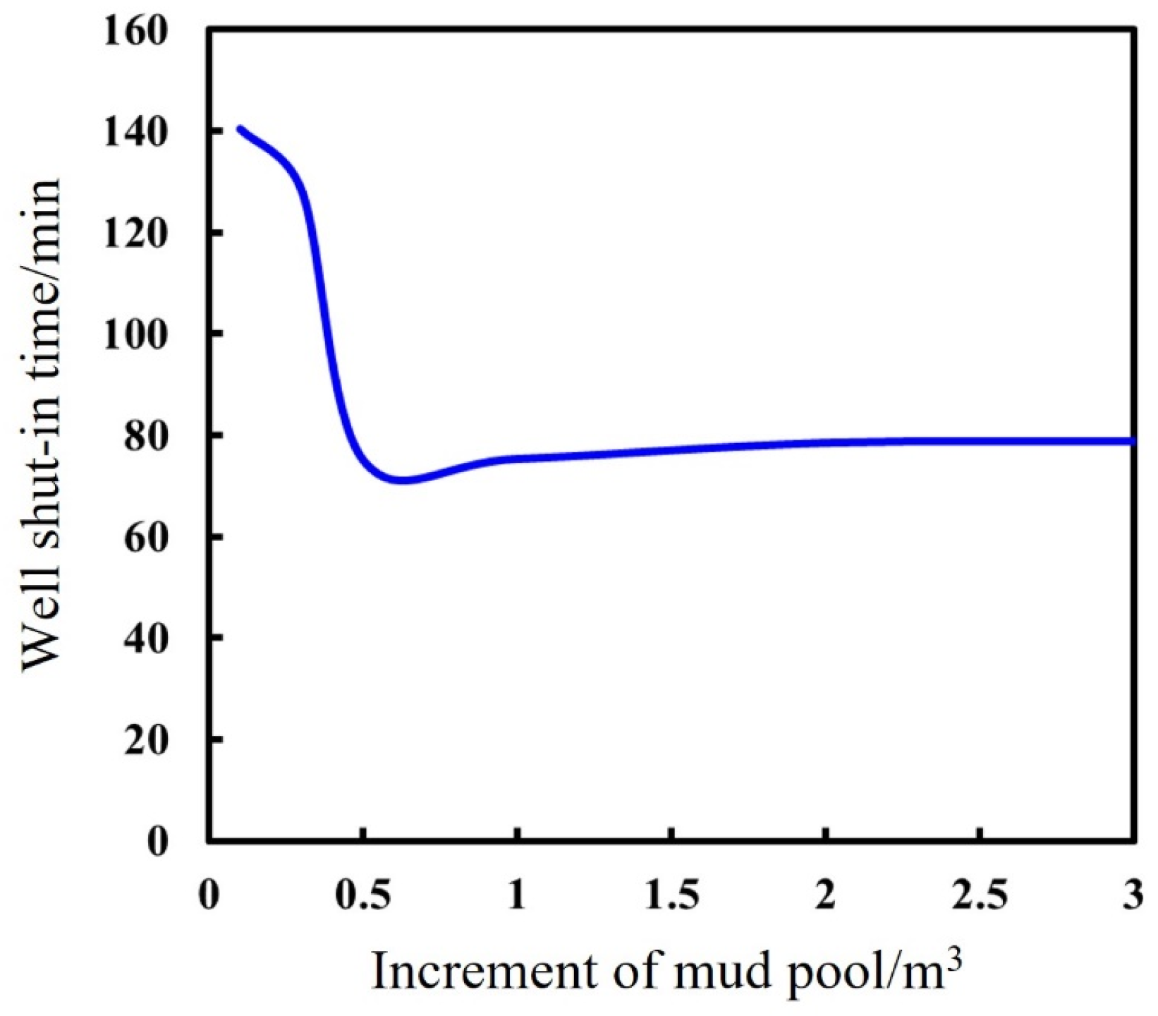
Figure 14 shows the curves of the recommended shut-in time (wellbore pressure rise to formation pressure) for different mud-pool increments. The simulation showed that the recommended shut-in time did not change significantly when the mud-pool increment exceeded 0.5 m
3. The recommended shut-in time decreased from 140.54 min to 78.81 min when the mud-pool increment increased from 0.1 m
3 to 3 m
3.
3.3.3. Analysis of Well Shut-In Pressures at Different Bottomhole Differential Pressures
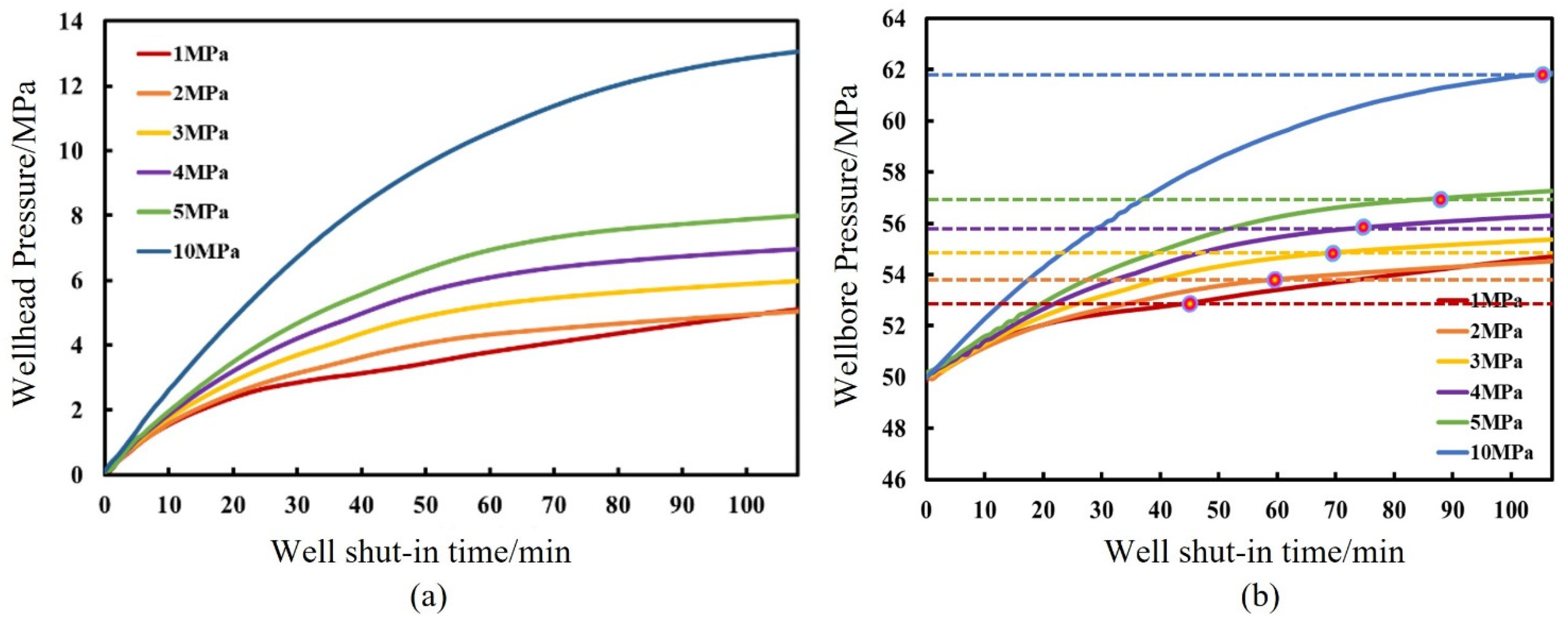
Figure 15a,b show the variations in the shut-in jacket and bottomhole pressures with shut-in time under different bottomhole differential pressure shut-in conditions. The higher the wellbore differential pressure at the time of overflow, the faster the gas intrusion rate driven by the differential pressure, the faster the wellbore pressure recovery, and the higher the wellhead back pressure and wellbore pressure after the same time of well shut-in.
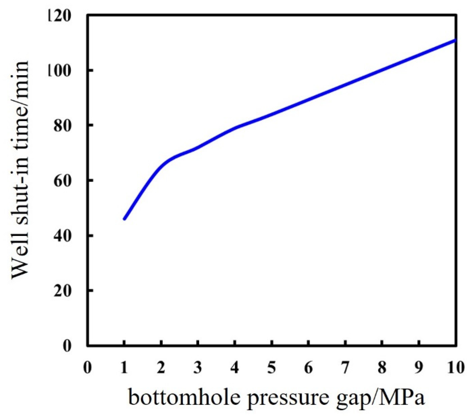
Figure 16 shows the recommended well shutdown time curves for different bottomhole differential pressures, which show that the recommended well shutdown time was prolonged with an increase in the bottomhole differential pressure at the time of overflow. The recommended well shutdown time increased from 46 to 111 min when the bottomhole differential pressure increased from 1 to 10 MPa.
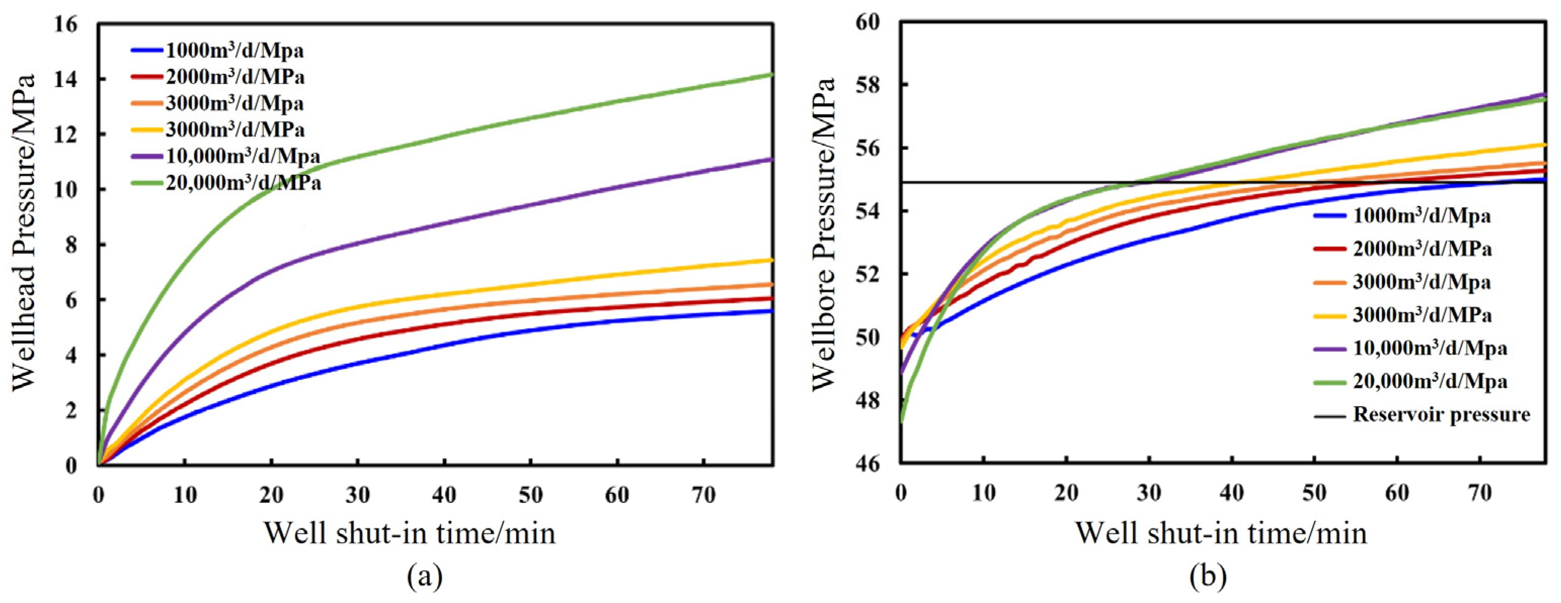
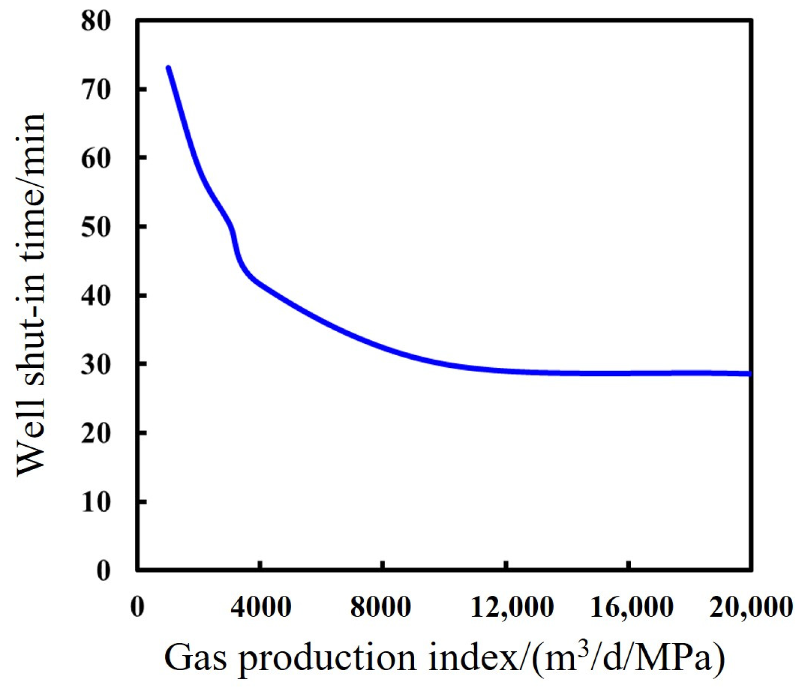
3.3.4. Analysis of Well Shut-In Pressures with Different Gas Production Indices
Figure 17a,b shows the changes in the shut-in casing pressure and bottomhole pressure with shut-in time under different gas production index shut-in conditions. The larger the gas production index, the faster the bottomhole gas inlet rate, and the more rapidly the gas is transported upward and expanded, resulting in a faster recovery of the wellbore pressure.
Figure 18 shows the recommended shut-in time curves under different gas production indices. The simulation showed that the recommended shut-in time decreased from 73.2 to 28.6 min when the gas production index increased from 1000 to 20,000 m
3/day/MPa.
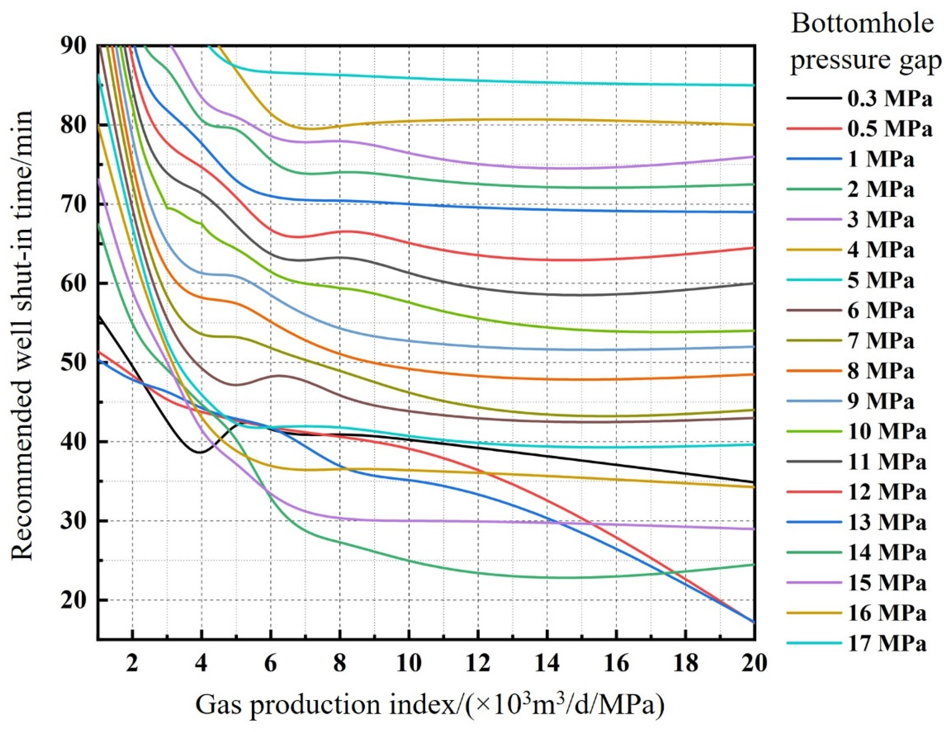
3.4. Deepwater Drilling Shut-In Wells for Pressure Plate
According to the overflow situation of the BY 5-2-1 well, under a mud-pool increment of 4 bbl (0.64 m
3), combined with the shut-in pressure model, the recommended shut-in times under different gas production indices and bottomhole differential pressures were simulated, and the shut-in pressure graphic plate of the BY 5-2-1 well was plotted, as shown in
Figure 19. The well shut-in time was determined based on the formation information estimated in the field. The graphical plate showed that the shut-in time of the BY 5-2-1 well should not be less than 15 min in any possible situation, and the recommended shut-in time could be up to 90 min in the case of a smaller gas production index and larger bottomhole differential pressure.
4. Conclusions
(1) The multi-gradient composite heat transfer mechanism of a formation-wellbore wall-annulus-drill pipe and the forced convection heat transfer characteristic of the annulus were considered along with the fluid intrusion of a complex formation and its transportation and distribution mechanism in the wellbore. A prediction model for the temperature and pressure field of the shut-in of deepwater drilling wells considering heat-fluid-solid coupling was established.
(2) By applying the established model, the transient shut-in process of deepwater drilling wells was analyzed and verified using the measured data. It was found that the average error of the set pressure rise during the shut-in process was 5.42%, which proved that the model predicted well shut in pressure very effectively.
(3) The thermal expansion of the fluid led to a decrease in the fluid density, and the higher the wellhead back pressure after shutting off the well for the same period of time, the higher the temperature gradient of the formation. The influence of temperature change on pressure recovery was predicted.
(4) The shut-in pressure-seeking time required to recover the wellbore pressure to the formation pressure after shutting down the well showed nonlinear variations with the mud-pool increment, formation pressure, gas production index, and other factors.
(5) A deepwater drilling well shut-in pressure-seeking template was determined. The recommended shut-in time for deepwater drilling wells should not be less than 15 min and should be more than 90 min in the case of a small gas production index and a large bottomhole pressure difference.
(6) We will continue to validate the accuracy of the model as a way to increase its generalizability by collecting information from different types of wells.


