
Physical Modeling of a Water Hydraulic Proportional Cartridge Valve for a Digital Twin in a Hydraulic Press Machine


Abstract
1. Introduction
2. Device and Operation
3. Modeling
3.1. Physical Model
- 1.
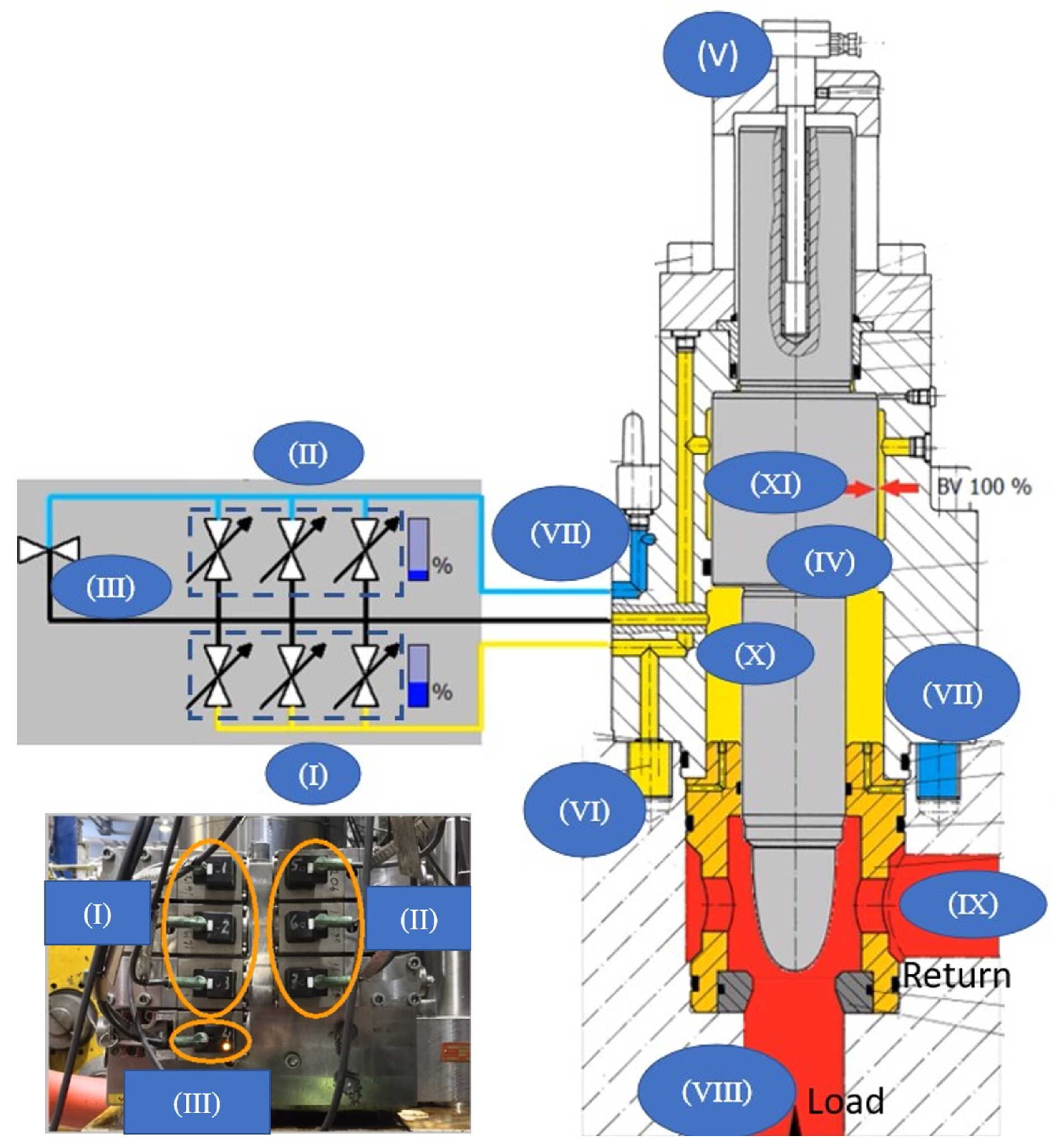
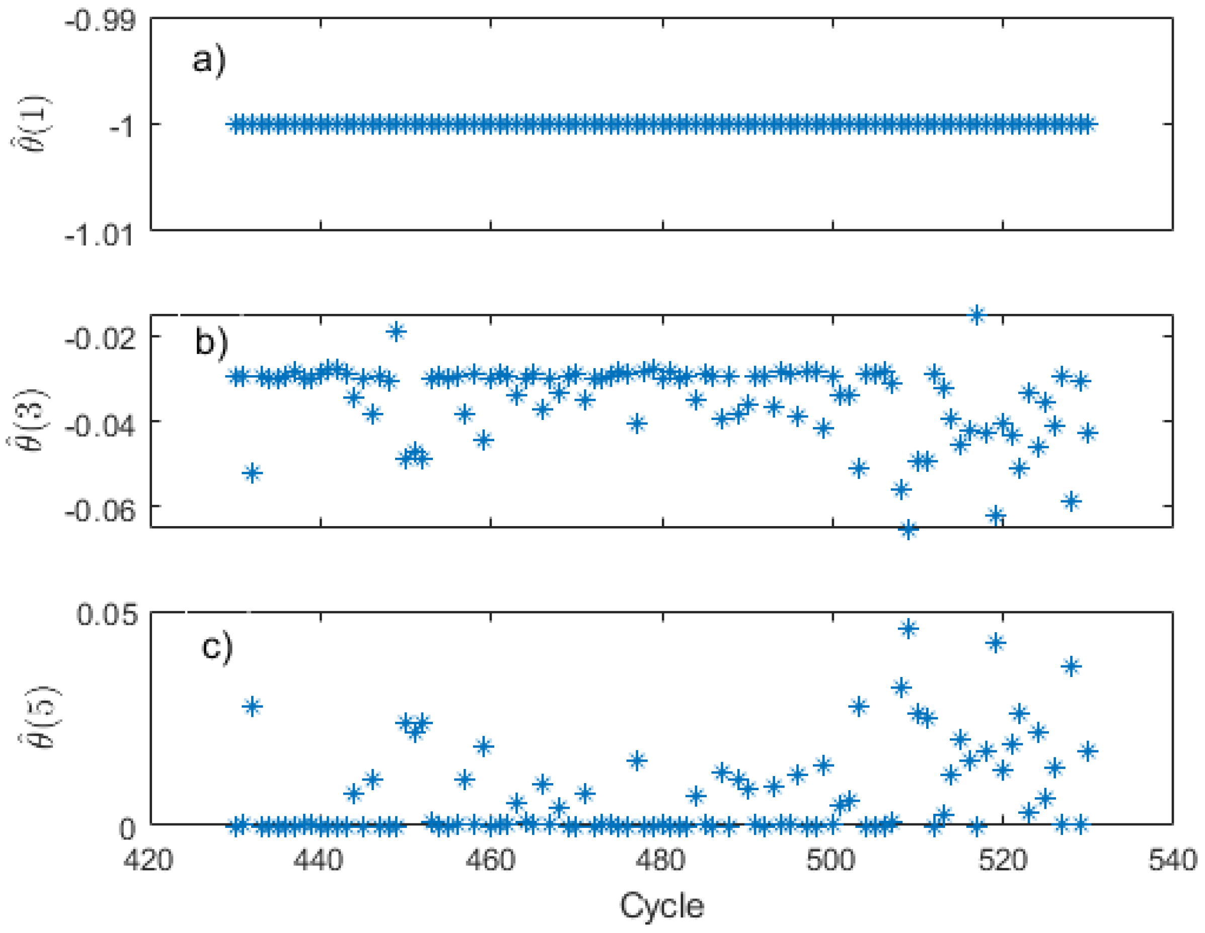
- Pilot valve model (I and II): These pilot valves consist of a solenoid, its armature, and a pre-loaded spring. Equations (3.6) and (3.7) in [11] describe a third-order coupled system, which, in this case, is the dynamics of the armature and the electrical circuit of the coil. We assume that the time constants of the armature’s motion are much smaller than those of the spindle’s motion. Therefore, we neglect the inductance of the coil’s circuit, the linear momentum, the viscous force, the flow forces acting on the armature, and the induced electromagnetic force from the armature’s motion. The last one is allowed because the electromagnetic force on the armature was greater; as such, we obtainfor valve i, where . In this case, (see Figure 1). By setting for to derive , we obtainwhere . assumes as the offset of , which is assumed to be the same for all pilot valves (see Figure 3b). All pilot valves are of the same type.
- 2.
- Volumetric flow rate of the pilot valves (I and II): The standard Equation (4.1) in [11] is used to describe the flow (which assumed the fluid was incompressible with a high Reynolds number (i.e., laminar flow)). As such, we obtainwhere is the discharge flow area when assuming a rectangular section, which depends on the voltage applied to the coil of the pilot valve i. for , and for . We substitute j by subindexing for , as well as by subindexing for , i.e., and control for and , respectively.
- 3.
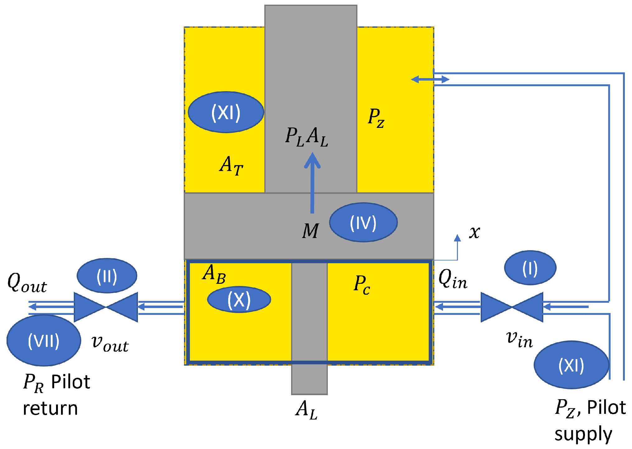
- The deformable volume (X) of the main valve is chosen as the control volume, as indicated by the solid blue line in Figure 2. The change in the control volume is understood as a function of the spindle’s position. For an incompressible fluid, the continuity Equation (5.5) in [33] becomesThe flow of the pilot valves of group (I), i.e., , increases the volume of the lower chamber (X), whereas the flow of those of group (II), i.e., , decreases the same volume. The contribution of the assumption of water being incompressible to the modeling errors is analyzed in detail in Section 4.2.
- 4.
- The spindle (IV) equation of motion of the main valve determines the motion of the main valve’s spindle, which iswhen or . For a marginally stable valve, as with the one under study, there is no spring; hence, no term was proportional to x. is the force exerted by the flow going from (VIII) to (IX) in Figure 1. An analysis of the flow forces allows for the term to appear in the equation. is the force given by the main valve’s spindle mass. We assume that the Coulomb friction term can be neglected relative to and due to a difference of 3–5 orders of magnitude when assuming friction between steel and rubber, i.e., the seal’s material. Furthermore, as we have values of (cf. scale of Figure 3c,d) and (cf. Figure 2), we thus obtaine , as well as . The flow forces can be described bywhich can be obtained after deriving and linearizing with respect to x and (see Equation (4.20) in [11]). The subscript “o” signifies the nominal operating conditions of the valve. Considering the control volume, as illustrated in Figures 4–21 by dashed lines and the dimension given in Equation (4.122), both in [11], as well as the operating conditions of the hydraulic valve under study, we consider to be negligible relative to and . This is because there is a difference of two orders of magnitude. More information about how to derive the expression of the coefficients in (6) can be found in Chapter 4, more specifically in Sections 4.3 and 4.6, in [11]. Finally, we obtain the main valve’s spindle equation of motion, which is
- 5.
- Approximation of in the main valve (X): Since is not measured, it is derived from Equations (3) and (4). Furthermore, knowing that the pilot valves are identical, and that is applied to all of the coils of pilot valves (I) and to (II) (see Figure 1 and Equation (4)), we obtainwhere and . For , we use the auxiliary functionand for , we usewhich are derived from Equation (3). and are approximated by a Taylor series in around the operating point , which is the equilibrium point of Equation (7). By performing this, keeping the linear terms, and substituting these in Equation (8), we obtainwhereIn the above, is the first derivative of , which is evaluated at ; is the first derivative of ; ; and .
- 6.
- The auxiliary function is approximated by a Taylor series in and around and , respectively, where , . We keep the linear terms and Equation (13) is approximated bywherewhere , is the derivative of with respect to , and is the derivative of with respect to . Indeed, both are evaluated at . The sign of each of the parameters is specified explicitly in Equation (15), and this is performed in accordance with the physics of the device described in Equations (1)–(13). is positive or negative depending on . Notice that Equation (14) is a non-linear input–output model and linear in terms of the parameters. The non-linearities are related to , , , and . These terms are obtained from the square root in and the product in Equation (3).
3.2. Parameter Estimation
3.3. Model Validation
4. Results and Discussion
4.1. Physical Model
4.2. Modeling Errors
4.3. Aging
5. Conclusions
Supplementary Materials
Author Contributions
Funding
Data Availability Statement
Conflicts of Interest
Nomenclature
| () | Cross-sectional area of spindle (IV) in contact with fluid in (XI) () |
| () | Cross-sectional area of spindle (IV) in contact with fluid in (X) () |
| () | Cross-sectional area of the spindle (IV) in contact with fluid that goes from (VIII) to (IX) () |
| (M) | Mass of the spindle (IV) () |
| () | Pressure of the fluid in (VI) and the upper chamber (XI) () |
| () | Pressure of the fluid in the reservoir (VII) () |
| () | Pressure of the fluid in the lower chamber (X) () |
| () | Pressure of the fluid in (IX) () |
| () | Volumetric flow rate of the pilot valves (i = ) () |
| () | Voltage applied to the pilot valve coil ( (normalized) |
| () | Voltage applied to the pilot valve coils in group (I) (normalized) |
| () | Voltage applied to the pilot valve coils in group (II) (normalized) |
| (x) | Position of the main spindle (IV) (normalized) |
| (g) | Gravity () |
| (t) | Time () |
| (m) | Number of pilot valves in Group (I) |
| (l) | Number of pilot valves in group (II) |
| (k) | Spring rate of pilot valves in group (I) and (II) () |
| () | Armature position of valve i () (m) |
| () | Magnetic coupling coefficient of pilot valves in group (I) and (II) () |
| () | Maximum supplied voltage to the pilot valve coil () |
| (R) | Resistance of the pilot valve coil () |
| () | Pre-load force of the spring () |
| () | Offset of ( (normalized)) |
| () | Discharge coefficient |
| () | Fluid density () |
| () | Pressure drop of the pilot valves in group (I) and (II) () () |
| () | Speed of the spindle (IV) () |
| () | Acceleration of the spindle (IV) () |
| (B) | Viscous drag coefficient () |
| () | Coulomb friction () |
| () | Flow force () |
| () | Flow gain coefficient () |
| () | Pressure flow coefficient () |
| () | Flow force gain () |
| () | Pressure flow force gain () |
| () | Maximum position of the spindle (IV) () |
| (T) | Sampling time () |
| (n) | Time (integer) |
| (N) | Number of samples |
| (f) | Frequency () |
References
- Tao, F.; Zhang, H.; Liu, A.; Nee, A.Y. Digital twin in industry: State-of-the-art. IEEE Trans. Ind. Inform. 2018, 15, 2405–2415. [Google Scholar] [CrossRef]
- Wright, L.; Davidson, S. How to tell the difference between a model and a digital twin. Adv. Model. Simul. Eng. Sci. 2020, 7, 1–13. [Google Scholar] [CrossRef]
- Roy, R.B.; Mishra, D.; Pal, S.K.; Chakravarty, T.; Panda, S.; Chandra, M.G.; Pal, A.; Misra, P.; Chakravarty, D.; Misra, S. Digital twin: Current scenario and a case study on a manufacturing process. Int. J. Adv. Manuf. Technol. 2020, 107, 3691–3714. [Google Scholar] [CrossRef]
- He, B.; Bai, K.J. Digital twin-based sustainable intelligent manufacturing: A review. Adv. Manuf. 2021, 9, 1–21. [Google Scholar] [CrossRef]
- Rituraj, R.; Scheidl, R. Towards digital twin development of counterbalance valves: Modelling and experimental investigation. Mech. Syst. Signal Process. 2023, 188, 110049. [Google Scholar] [CrossRef]
- Xiang, F.; Zhi, Z.; Jiang, G. Digital twins technolgy and its data fusion in iron and steel product life cycle. In Proceedings of the 2018 IEEE 15th International Conference on Networking, Sensing and Control (ICNSC), Zhuhai, China, 27–29 March 2018; pp. 1–5. [Google Scholar]
- Karandaev, A.S.; Gasiyarov, V.R.; Radionov, A.A.; Loginov, B.M. Development of digital models of interconnected electrical profiles for rolling–drawing wire mills. Machines 2021, 9, 54. [Google Scholar] [CrossRef]
- Gasiyarova, O.A.; Karandaev, A.S.; Erdakov, I.N.; Loginov, B.M.; Khramshin, V.R. Developing digital observer of angular gaps in rolling stand mechatronic system. Machines 2022, 10, 141. [Google Scholar] [CrossRef]
- Gonzalez, O.B.; Rönnow, D. Time series modelling of a radial-axial ring rolling system. Int. J. Model. Identif. Control 2023, 43, 13–25. [Google Scholar] [CrossRef]
- Gonzalez, O.B.; Rönnow, D. A Study of OBF-ARMAX Performance for Modelling of a Mechanical System Excited by a Low Frequency Signal for Condition Monitoring. In Proceedings of the European Workshop on Advanced Control and Diagnosis, Nancy, France, 16–18 November 2022; Springer: Cham, Switzerland, 2022; pp. 73–82. [Google Scholar]
- Manring, N.D.; Fales, R.C. Hydraulic Control Systems; John Wiley & Sons: Hoboken, NJ, USA, 2019. [Google Scholar]
- Han, M.; Liu, Y.; Wu, D.; Tan, H.; Li, C. Numerical analysis and optimisation of the flow forces in a water hydraulic proportional cartridge valve for injection system. IEEE Access 2018, 6, 10392–10401. [Google Scholar] [CrossRef]
- Liu, Z.; Li, L.; Yue, D.; Wei, L.; Liu, C.; Zuo, X. Dynamic Performance Improvement of Solenoid Screw-In Cartridge Valve Using a New Hybrid Voltage Control. Machines 2022, 10, 106. [Google Scholar] [CrossRef]
- Xu, B.; Shen, J.; Liu, S.; Su, Q.; Zhang, J. Research and development of electro-hydraulic control valves oriented to industry 4.0: A review. Chin. J. Mech. Eng. 2020, 33, 1–20. [Google Scholar] [CrossRef]
- Tamburrano, P.; Plummer, A.R.; Distaso, E.; Amirante, R. A review of electro-hydraulic servovalve research and development. Int. J. Fluid Power 2018, 20, 53–98. [Google Scholar] [CrossRef]
- Liu, S.; Yao, B. Energy-saving control of single-rod hydraulic cylinders with programmable valves and improved working mode selection. SAE Trans. 2002, 111, 51–61. [Google Scholar]
- Liu, S.; Yao, B. Adaptive robust control of programmable valves with manufacturer supplied flow mapping only. In Proceedings of the 2004 43rd IEEE Conference on Decision and Control (CDC)(IEEE Cat. No. 04CH37601), Nassau, Bahamas, 14–17 December 2004; Volumne 1, pp. 1117–1122. [Google Scholar]
- Liu, S.; Yao, B. On-board system identification of systems with unknown input nonlinearity and system parameters. In Proceedings of the ASME International Mechanical Engineering Congress and Exposition, Orlando, FL, USA, 5–11 November 2005; Volume 42169, pp. 1079–1085. [Google Scholar]
- Liu, S.; Yao, B. Automated onboard modeling of cartridge valve flow mapping. IEEE/ASME Trans. Mechatron. 2006, 11, 381–388. [Google Scholar]
- Lu, L.; Yao, B.; Liu, Z. Energy saving control of a hydraulic manipulator using five cartridge valves and one accumulator. IFAC Proc. Vol. 2013, 46, 84–90. [Google Scholar] [CrossRef]
- Xu, B.; Ding, R.; Zhang, J.; Su, Q. Modeling and dynamic characteristics analysis on a three-stage fast-response and large-flow directional valve. Energy Convers. Manag. 2014, 79, 187–199. [Google Scholar] [CrossRef]
- Yue, D.; Li, L.; Wei, L.; Liu, Z.; Liu, C.; Zuo, X. Effects of pulse voltage duration on open–close dynamic characteristics of solenoid screw-In cartridge valves. Processes 2021, 9, 1722. [Google Scholar] [CrossRef]
- Han, M.; Liu, Y.; Zheng, K.; Ding, Y.; Wu, D. Investigation on the modeling and dynamic characteristics of a fast-response and large-flow water hydraulic proportional cartridge valve. Proc. Inst. Mech. Eng. Part C J. Mech. Eng. Sci. 2020, 234, 4415–4432. [Google Scholar] [CrossRef]
- Ljung, L. System identification. In Signal Analysis and Prediction; Springer: Berlin/Heidelberg, Germany, 1998; pp. 163–173. [Google Scholar]
- Zhang, J.; Lu, Z.; Xu, B.; Su, Q. Investigation on the dynamic characteristics and control accuracy of a novel proportional directional valve with independently controlled pilot stage. ISA Trans. 2019, 93, 218–230. [Google Scholar] [CrossRef]
- Li, C.; Lyu, L.; Helian, B.; Chen, Z.; Yao, B. Precision motion control of an independent metering hydraulic system with nonlinear flow modeling and compensation. IEEE Trans. Ind. Electron. 2021, 69, 7088–7098. [Google Scholar] [CrossRef]
- Lu, Z.; Zhang, J.; Xu, B.; Wang, D.; Su, Q.; Qian, J.; Yang, G.; Pan, M. Deadzone compensation control based on detection of micro flow rate in pilot stage of proportional directional valve. ISA Trans. 2019, 94, 234–245. [Google Scholar] [CrossRef] [PubMed]
- Li, Y.; Wang, Q. Adaptive robust tracking control of a proportional pressure-reducing valve with dead zone and hysteresis. Trans. Inst. Meas. Control 2018, 40, 2151–2166. [Google Scholar] [CrossRef]
- Folgheraiter, M. A combined B-spline-neural-network and ARX model for online identification of nonlinear dynamic actuation systems. Neurocomputing 2016, 175, 433–442. [Google Scholar] [CrossRef]
- Tørdal, S.S.; Klausen, A.; Bak, M.K. Experimental system identification and black box modeling of hydraulic directional control valve. Model. Identif. Control 2015, 36, 225–235. [Google Scholar] [CrossRef]
- Kilic, E.; Dolen, M.; Koku, A.B.; Caliskan, H.; Balkan, T. Accurate pressure prediction of a servo-valve controlled hydraulic system. Mechatronics 2012, 22, 997–1014. [Google Scholar] [CrossRef]
- Alimonti, C. Experimental characterization of globe and gate valves in vertical gas–liquid flows. Exp. Therm. Fluid Sci. 2014, 54, 259–266. [Google Scholar] [CrossRef]
- Munson, B.R.; Okiishi, T.H.; Huebsch, W.W.; Rothmayer, A.P. Fluid Mechanics; Wiley: Singapore, 2013. [Google Scholar]
- Atkinson, K. An Introduction to Numerical Analysis; John Wiley & Sons: Hoboken, NJ, USA, 1991. [Google Scholar]
- Boyd, S.P.; Vandenberghe, L. Convex Optimization; Cambridge University Press: Cambridge, MA, USA, 2004. [Google Scholar]
- Grant, M.; Boyd, S.; Ye, Y. CVX: Matlab Software for Disciplined Convex Programming, version 2.0 Beta. 2009. Available online: https://cvxr.com/cvx (accessed on 10 March 2024).
- Grant, M.C.; Boyd, S.P. Graph implementations for nonsmooth convex programs. In Recent Advances in Learning and Control; Springer: London, UK, 2008; pp. 95–110. [Google Scholar]
- Stoica, P.; Söderström, T. System Identification; Prentice-Hall International: Upper Saddle River, NJ, USA, 1989. [Google Scholar]
- Wasserman, L. All of Statistics: A Concise Course in Statistical Inference; Springer: Berlin/Heidelberg, Germany, 2004; Volume 26. [Google Scholar]


| Description | ||||
|---|---|---|---|---|
| −1.16 | −1.24 | −0.99 | ||
| - | - | |||
| - | ||||
| MSE training | ||||
| MSE test |
| Parameter | Units |
|---|---|
| , , , |
| M | 65–100 |
| B | 1000–4500 |
| – | |
| 0.95–0.97 | |
| 1000 | |
| 0.8–1 | |
| – | |
| 0.5–0.7 | |
| 3 × |
| Interval | ||
|---|---|---|
| −0.99 | – | |
| – | ||
| – | ||
| 0.01–0.6 |
| Description | |||||
|---|---|---|---|---|---|
| (a) | |||||
| (b) | |||||
| (c) | |||||
| (d) | |||||
| (e) | |||||
| (f) | |||||
| (g) | Euler forward method | ||||
| (h) | Approx. (9) and (10) | - | |||
| (i) | Approx. (12) | ||||
| (j) | Approx. (9), (10), and (12) | - | |||
| (k) | Compressibility | ||||
| Total |
Disclaimer/Publisher’s Note: The statements, opinions and data contained in all publications are solely those of the individual author(s) and contributor(s) and not of MDPI and/or the editor(s). MDPI and/or the editor(s) disclaim responsibility for any injury to people or property resulting from any ideas, methods, instructions or products referred to in the content. |
© 2024 by the authors. Licensee MDPI, Basel, Switzerland. This article is an open access article distributed under the terms and conditions of the Creative Commons Attribution (CC BY) license (https://creativecommons.org/licenses/by/4.0/).
Share and Cite
Bautista Gonzalez, O.; Rönnow, D. Physical Modeling of a Water Hydraulic Proportional Cartridge Valve for a Digital Twin in a Hydraulic Press Machine. Processes 2024, 12, 693. https://doi.org/10.3390/pr12040693
Bautista Gonzalez O, Rönnow D. Physical Modeling of a Water Hydraulic Proportional Cartridge Valve for a Digital Twin in a Hydraulic Press Machine. Processes. 2024; 12(4):693. https://doi.org/10.3390/pr12040693
Chicago/Turabian StyleBautista Gonzalez, Oscar, and Daniel Rönnow. 2024. "Physical Modeling of a Water Hydraulic Proportional Cartridge Valve for a Digital Twin in a Hydraulic Press Machine" Processes 12, no. 4: 693. https://doi.org/10.3390/pr12040693
APA StyleBautista Gonzalez, O., & Rönnow, D. (2024). Physical Modeling of a Water Hydraulic Proportional Cartridge Valve for a Digital Twin in a Hydraulic Press Machine. Processes, 12(4), 693. https://doi.org/10.3390/pr12040693