A Matrix Completion Method for Imputing Missing Values of Process Data

Abstract

Real-time process data are the foundation for the successful implementation of intelligent manufacturing in the chemical industry. However, in the actual production process, process data may randomly be missing due to various reasons, thus affecting the practical application of intelligent manufacturing technology. Therefore, this paper proposes the application of appropriate matrix completion algorithms to impute the missing values of real-time process data. Considering the characteristics of online missing value imputation problems, this paper proposes an improved method for a matrix completion algorithm that is suitable for real-time missing data imputation. By utilizing real device data, this paper studies the impact of algorithm parameters on the effect of missing value imputing and compares it with several classical missing value imputing methods. The results show that the introduced method achieves higher accuracy in data imputation compared to the baseline method. Furthermore, the proposed enhancement significantly improves the speed performance of algorithms.

1. Introduction

As intelligent manufacturing in the chemical industry gains momentum, the significance of real-time process data escalates. However, transmission interruptions, sensor failures, or database issues may cause random missing data in real-time process data during the actual production process [1], thereby reducing the representativeness of real-time data and affecting the implementation of intelligent manufacturing in the chemical industry [2]. Therefore, the imputation of missing values is critically essential for the successful execution of intelligent manufacturing within the chemical industry.

We commonly use three methods for the analysis of data with missing values: the deletion method, the imputation method, and the model-based method [3]. Commonly used deletion methods for handling missing data include listwise and pairwise. Listwise deletion involves removing all data associated with time points that exhibit anomalies. This method may lead to the deletion of significant amounts of data, thus diminishing statistical efficiency and potentially introducing more uncertainty and bias into parameter estimates [4]. On the other hand, pairwise deletion may lead to inconsistent data lengths due to the varying time points of the deleted data, making it impossible to reconstruct and represent the complete dataset as a matrix. This inconsistency affects the application of numerous algorithms, complicating subsequent tasks in process modeling and statistical inference for monitoring.

The data processed using deletion methods are illustrated in Figure 1.

Thus, when a significant amount of data is missing and the correlation between variables is affected, it is not advisable to use deletion methods. To maximize the number of samples and preserve statistical characteristics for subsequent data mining, it is advisable to employ the strategy of estimating and imputing missing data. While manually selecting values for imputation is possible, automated methods become indispensable for processing the real-time data involved in the deployment of intelligent manufacturing [5]. Common strategies for imputation involve using statistical values, such as the mean or median values of variables [6], or employing a similar pattern from complete data, such as hot-deck imputation [2]. Model-based methods often involve algorithms, such as the Maximum Likelihood (ML) algorithm [7] and the Expectation-Maximization (EM) algorithm [8].

To address the issue of missing values in chemical process data, this paper employs a method from machine learning: the Matrix Completion Method (MCM). Due to its remarkable ability to discover and leverage latent patterns or structures, the MCM has found applications in recommendation systems, image restoration, analytical chemistry, thermodynamics, and quantum chemistry. In chemical engineering, the MCM has been used to predict the thermodynamic properties and the models of mixtures. For example, it has been incorporated into the UNIQUAC model to predict activity coefficients at any temperature and composition, surpassing the performance of the best physical models for predicting activity coefficients [9]. Additionally, the MCM has been used to predict Henry’s law coefficients based on the sparsity of experimental data matrices, outperforming traditional state equations [10]. It has also found application in calculations involving quantum and variational effects [11].

This paper will introduce existing methods for imputing missing data in Section 2. Section 3 briefly introduces the principle of matrix completion and improves the existing Matrix Completion Method according to the characteristics of the online data imputing problem. Section 4 will evaluate the efficacy of the MCM in processing missing data, thus providing a comparative discussion with other methods. Finally, Section 5 concludes this study.

2. Established Methods for Data Imputation

In handling chemical process data, routine methods for imputing missing values involve utilizing existing data for imputation or employing model-based methods. The former includes mean imputation, median imputation, and hot-deck imputation. These methods aim to recover or estimate missing data values based on available information, thus enhancing the accuracy of portraying the genuine characteristics of the data for further analysis and exploration. The latter encompasses various model-based methods, including the ML and EM algorithms. These methods impute missing values by establishing models and generating data that adhere to specific distributions for imputation. The selection of each method depends on the particular data characteristics and analytical requirements.

2.1. Mean and Median Replacement

Imputing missing data using the mean of data from different time points on the same sensor offers fast processing speed. Let ${\overline{x}}_{\mathrm{obs}}$ represent the mean of the observed data. The missing data $x_{\mathrm{mis}}$ are formulated as follows:

$$x_{\mathrm{mis}}={\overline{x}}_{\mathrm{obs}}$$

(1)

Imputing missing data using the median of data from different time points on the same sensor provides a processing speed similar to mean imputation. Let $M{e}_{\mathrm{obs}}$ represent the median of the observed data. The missing data $x_{\mathrm{mis}}$ are given by:

$$x_{\mathrm{mis}}=M{e}_{\mathrm{obs}}$$

(2)

2.2. Hot-Deck Replacement

The hot-deck imputation method for processing missing data involves identifying an object in the existing data that is most similar to the missing data and then imputing the missing values with the values from this similar object. In defining similarity, this experiment treats the data obtained from each time point as individual entities. Comparing the absolute average differences in the observed data $x_{\mathrm{obs}}$ among different entities serves as the measure for determining similarity. Assuming there are $n$ sensors of observed data from time point 1 and time point 2, we can express their level of similarity $X_s$ as follows:

$$X\mathrm{s}=\frac{{\displaystyle \sum \left|x_{\mathrm{obs1}}-x_{\mathrm{obs2}}\right|}}{n}$$

(3)

When $X_s$ is small, indicating a higher level of similarity, the strategy involves using $x_{\mathrm{obs2}}$ from time point 2 to impute the missing data $x_{\mathrm{mis1}}$ for time point 1.

$$x_{\mathrm{mis1}}=x_{\mathrm{obs2}}$$

(4)

2.3. Model-Based Methods

Model-based methods include ML (Maximum Likelihood) and EM (Expectation-Maximization) algorithms. The ML algorithm assumes that we have a dataset $X$ with a distribution described by parameters Θ. The parameter Θ is dictated by the statistical distribution of the data. Given observed data $x_{\mathrm{obs}}$ and missing data $x_{\mathrm{mis}}$, the marginal probability density of $x_{\mathrm{obs}}$ is defined as follows:

$$P(x_{\mathrm{obs}}|\mathsf{\Theta })={\displaystyle \int P(x_{\mathrm{obs}},x_{\mathrm{mis}}|{\mathsf{\Theta }}^{(m)})}d{x}_{\mathrm{mis}}$$

(5)

The likelihood definition of Θ based on $x_{\mathrm{obs}}$ is as follows:

$$L(x_{\mathrm{obs}}|\mathsf{\Theta })\propto P(x_{\mathrm{obs}}|\mathsf{\Theta })$$

(6)

If the likelihood function is differentiable and Θ is known, the estimate of $x_{\mathrm{mis}}$ can be obtained by solving the problem illustrated in Equation (7):

$$\frac{\partial \log [L(Y_{\mathrm{obs}}|\mathsf{\Theta })]}{\partial \mathsf{\Theta }}=0$$

(7)

The EM algorithm consists of two steps: an E-step and an M-step. In the E-step, the expectation of the log-likelihood function is calculated. This expectation is equivalent to the conditional distribution of $x_{\mathrm{mis}}$ given $x_{\mathrm{obs}}$ under the estimation of Θ^(m), and it is expressed as follows:

$$E(x_{\mathrm{mis}}|x_{\mathrm{obs}},{\mathsf{\Theta }}^{(m)})=E[\log L(x_{\mathrm{obs}},x_{\mathrm{mis}}|{\mathsf{\Theta }}^{(m)})]$$

(8)

During the M-step, the goal is to determine the parameters Θ^(m+1) that maximize the expectation E. The formula is given by:

$${\mathsf{\Theta }}^{(m+1)}=\underset{\mathsf{\Theta }}{\arg \max }E(\mathsf{\Theta }|{\mathsf{\Theta }}^{(m)})$$

(9)

The EM algorithm iterates between these two steps until the estimated values converge.

The methods previously discussed, such as mean and median imputation, are simple to calculate but lack accuracy. These methods do not utilize information beyond the data collected by the current sensor, leading to inefficient utilization of information. Hot-deck imputation utilizes information beyond the current sensor. It still uses existing values to impute missing ones, potentially resulting in a single observed value being used to impute multiple time points. For real-time data, it is difficult for us to predict their distribution in advance, and the formulation of the likelihood function in the ML algorithm becomes complex to derive without a definite data distribution. While the EM algorithm does not require the likelihood function expression, it still assumes a specific data distribution and has a slow computation speed.

The MCM can effectively address the issues with the previously mentioned algorithms. The MCM leverages the hidden relationships within the data to calculate new values for imputing missing ones, thus eliminating the need to derive expressions or make assumptions about data distribution.

3. Data Imputation with Improved Matrix Completion Methods

3.1. Principles of Matrix Completion

Matrix completion problems can be considered a type of matrix recovery problem. Specifically, they involve restoring the missing elements in the matrix based on a limited number of known elements [12,13]. Typical applications include estimating missing data, generating recommendations, uncovering hidden structures, conducting image restoration, and classification [14,15,16].

Matrix completion aims to recover the entire matrix using a limited amount of observed data. We record the positions of the observed data with Ω and search for a matrix X that has the same values as the input data matrix M at the known positions and has the minimum rank. Low-rank matrices preserve a substantial amount of redundant information, which we can use to recover the missing data in the matrix. The operator P_Ω sets all elements not in Ω in the matrix to zero, and the elements in Ω are P_Ω (X) = X. Therefore, we can formulate the above problem as follows:

$$\underset{X}{\mathrm{minimize}} \mathrm{rank}(X), \mathrm{s}.\mathrm{t}. P_{\mathsf{\Omega }}(X)=P_{\mathsf{\Omega }}(M)$$

(10)

However, the previously discussed problem is an NP-hard problem [17], which is computationally complex and difficult to solve directly. Consequently, it requires replacement with a problem that is easier to solve.

There are various models for matrix completion. These include, for example, models based on nuclear norm relaxation, in which Ma [18] and Toh [19] relaxed the standard problem into a matrix LASSO model. Additionally, the SVT algorithm proposed by Cai et al. [20] enhances the stability of solving matrix completion problems. Another model is based on matrix factorization. For example, the SOR algorithm proposed by Wen et al. [21] can handle large-scale matrix completion problems faster than traditional nuclear norm minimization algorithms. However, this approach requires an initial rank estimate, and due to the non-convex nature of the model, it cannot assure global convergence. Finally, models based on non-convex function relaxation are also an option. These include, for example, the algorithm proposed by Nie et al. [22] using Schatten p-norm and Lp-norm, and the FGSR algorithm proposed by Fan et al. [23]. Moreover, the FGSR algorithm avoids SVD decomposition, resulting in higher computational efficiency, and is insensitive to the choice of initial rank.

Due to the challenge of estimating the initial rank of the target data, this study selects the SVT (Singular Value Thresholding) algorithm, which does not require initial rank estimation, and the FGSR (Factor Group-Sparse Regularization) algorithm, which is not sensitive to the initial rank. We improve these algorithms by incorporating features for online use to impute missing values.

The SVT algorithm applies convex relaxation to the problem (10), transforming it into the following problem:

$$\underset{X}{\mathrm{minimize}}{‖X‖}_{*}, \mathrm{s}.\mathrm{t}. P_{\mathsf{\Omega }}(X)=P_{\mathsf{\Omega }}(M)$$

(11)

This optimization problem involves regularization, resulting in the construction of a Lagrangian function. Finally, we use the alternating iterative method to solve the optimization problem, expressing it in the following form:

$$\left\{\begin{array}{l}{X}^k=D_{\tau }(Y^{k-1})\\ Y^k=Y^{k-1}+{\delta }_k{P}_{\mathsf{\Omega }}(M-X^k)\end{array}\right.$$

(12)

In this context, $Y$ is the Lagrange multiplier, ${\delta }_k$ is the step size, and the operation $D_{\tau }(Y^{k-1})$ is represented by the following equation:

$$D_{\tau }(Y^{k-1})=\left\{\begin{array}{l}[U,S,V]=\mathrm{SVD}(Y^{k-1})\\ S=\mathrm{sgn}(S)\cdot \max (\left|S\right|-\tau ,0)\\ X^k=U\ast S\ast V^T\end{array}\right.$$

(13)

where ε is the convergence error, the condition for ending the iteration is:

$$\frac{{‖P_{\mathsf{\Omega }}(M-X^k)‖}_F}{{‖P_{\mathsf{\Omega }}M‖}_F}<\epsilon$$

(14)

The FGSR algorithm uses other parameters as proxies for rank, transforming problem (10) into the following form:

$$\underset{X}{\mathrm{minimize}} \mathrm{FGSR}(X), \mathrm{s}.\mathrm{t}. P_{\mathsf{\Omega }}(X)=P_{\mathsf{\Omega }}(M)$$

(15)

FGSR(X) can be expressed as follows:

$$\mathrm{FGSR}(X)=\frac{2}{3{\alpha }^{1/3}}\underset{AB=X}{\min }{‖A‖}_{2,1}+\frac{\alpha }{2}{‖B‖}_F^2$$

(16)

$A$ and $B$ can be represented as follows:

$$\left\{\begin{array}{l}[U_X,S_X,V_X]=\mathrm{SVD}(X)\\ A={\alpha }^{\frac{1}{3}}{U}_X{S}_X^{\frac{2}{3}}\\ B={\alpha }^{-\frac{1}{3}}{S}_X^{\frac{1}{3}}{V}_X^T\end{array}\right.$$

(17)

The problem can be represented as follows:

$$\underset{X}{\mathrm{minimize}}{‖A‖}_{2,1}+\frac{\alpha }{2}{‖B‖}_F^2, \mathrm{s}.\mathrm{t}. X=AB,P_{\mathsf{\Omega }}(X)=P_{\mathsf{\Omega }}(M)$$

(18)

We can solve the matrix completion problem by addressing the problem (18).

3.2. Data Imputation Based on Matrix Completion

The MCM is used to impute missing values within chemical processes. The fundamental principle is that data from chemical processes include control variable data $X_{\mathrm{con}}$ and display variable data $X_{\mathrm{var}}$. The data are in matrix form, with one dimension representing time and the other representing sensor identification. The display variable data $X_{\mathrm{var}}$ are returned after being collected by sensors at various positions in the production device, which include observed data $x_{\mathrm{obsv}}$ and missing data $x_{\mathrm{mis}}$ caused by transmission or sensor failure. Control variable data $X_{\mathrm{con}}$ are set manually and contain observed data $x_{\mathrm{obsc}}$. Consequently, the raw data can be perceived as a matrix $M$ with missing elements composed of $x_{\mathrm{obsv}}$, $x_{\mathrm{obsc}}$, and $x_{\mathrm{mis}}$. The form of matrix $M$ is shown in Figure 2.

From this perspective, the problem of filling in missing values in chemical process data can be transformed into a matrix completion problem, as follows:

$$X=fMCM(M)$$

(19)

Here, $X$ represents the dataset after filling, and the specific process of data processing is shown in Figure 3:

Given that the equipment in chemical plants operates continuously, generating a constant stream of new data, we have adopted a moving window strategy for online data cleansing in this study. A moving window can reduce the size of the input matrix, thereby accelerating the speed of matrix completion for data processing.

In terms of the selection of parameters used in the algorithm, considering the balance between accuracy and computation time, the convergence error ε of the algorithm is set to ε < 10⁻⁶, and the maximum number of iterations is set to 300.

The parameters of the SVT algorithm include the step size δ and the parameter τ. The conventional range of step size δ is 0~2, and this study uses the middle value δ = 1. And, the parameter τ is selected empirically, following reference [20]. The literature sets the parameter τ for an n × n matrix as 5n. In this study, for a matrix of size n₁ × n₂, the parameter τ is determined as 5 × qrt(n₁ × n₂).

For the FGSR algorithm, parameters include λ, d, and α. Step size λ is set at 0.3. Parameter d represents the rank of the factor matrix after matrix decomposition, and its selection range is d ≤ min (n₁, n₂), where n₁ and n₂ are the row and column numbers of the matrix. In this study, d = min (n₁, n₂). Parameter α, which adjusts the scale of the two-factor matrices following matrix decomposition, is chosen from the range α > 0. In this experiment, we set α = 2. The reasons for parameter selection refer to Section 4.3.

3.3. Improved Matrix Completion for Online Computing

In the application of the matrix completion algorithm, there is a need to initialize some data involved in the iterative computation. When processing data using a sliding window, most of the data in two adjacent windows are the same. Consequently, we consider using the data from the last iteration of the previous window’s computation as the initial data for the next window to reduce the number of iterative computations for the new window.

We posit that the data window currently under processing is the $i\mathrm{-th}$ window. The $D_{\tau }$ operation from Equation (13) of the SVT algorithm is improved, leading to the $D{n}_{\tau }$ operation, as shown in Equation (20).

$$D{n}_{\tau }(Y^{k-1})=\left\{\begin{array}{l}[U,S,V]=\mathrm{SVD}(Y^{k-1}), \mathrm{if} \mathrm{i}=1,3,5\dots \\ [U,S,V]=U^{i-1},S^{i-1},V^{i-1}, \mathrm{if} \mathrm{i}=2,4,6\dots \\ S=\mathrm{sgn}(S)\cdot \max (\left|S\right|-\tau ,0)\\ X^k=U\ast S\ast V^T\end{array}\right.$$

(20)

$U^{i-1}$, $S^{i-1}$, and $V^{i-1}$ represent the final iteration of the prior window. By implementing this improvement and capitalizing on the advantages of online processing, we minimize the number of SVD decompositions, thus lowering the overall time expenditure while ensuring precision. We will identify the SVT algorithm incorporating these changes as the ISVT (Improved Singular Value Thresholding) algorithm in the following text.

For the FGSR algorithm, we begin iterative computation upon each window transition and use $A_{i-1}$ and $B_{i-1}$ from the concluding iteration of the prior window when initializing matrices $A_i$ and $B_i$ for the $i-\mathrm{th}$ window’s computation ($i\ne 1$) according to (17). The modified initialization of $A$ and $B$ can be denoted by Equation (21).

$$\left\{\begin{array}{l}[A,B]=[A_{i-1},B_{i-1}], \mathrm{if} \mathrm{i}\ne 1\\ [U_X,S_X,V_X]=\mathrm{SVD}(X), \mathrm{if} \mathrm{i}=1\\ A={\alpha }^{\frac{1}{3}}{U}_X{S}_X^{\frac{2}{3}}\\ B={\alpha }^{\frac{1}{3}}{S}_X{V}_X^T\end{array}\right.$$

(21)

Such a practice can effectively decrease the frequency of SVD decompositions and accelerate the computational speed. In the subsequent sections, we will refer to the modified FGSR algorithm as the IFGSR (Improved Factor Group-Sparse Regularization) algorithm.

4. Performance Evaluations

4.1. Studied Case

The experimental data are derived from the DCS system of an atmospheric–vacuum distillation unit in a particular refinery. The atmospheric–vacuum distillation unit, an essential device that finds wide application in areas including petroleum and chemical engineering, plays a significant role in improving oil refining optimization and economic efficiency.

The DCS system records assorted data from the apparatus, including the feed temperature, tower top pressure, and side draw flow rate of the distillation column within the unit. The data referenced in this paper are logged every five minutes, with the initial data being complete. The initial data are divided into two groups: control variable data $X_{\mathrm{c}\mathrm{o}\mathrm{n}}$ and display variable data $X_{\mathrm{var}}$. The temperature (TI), pressure (PI), and flow rate (FI) data gathered by the DCS serve as display variable data $X_{\mathrm{var}}$, while the input data PIC, TIC, and FIC for the control system function as control variable data $X_{\mathrm{con}}$.

All data preprocessing and subsequent processing tasks are accomplished using MatlabR2021b. The program is operated on a laptop with a 3.20 GHz CPU and 16 GB of memory.

4.2. Evaluation Procedures

This study selects three common methods for processing missing values: mean imputation, median imputation, and hot-deck imputation. Additionally, four matrix completion algorithms, SVT, ISVT, FGSR, and IFGSR, are used to impute the missing values.

In the experiment, we selected data from 600 time points, which formed an original data matrix of size n_s × 600, where n_s represents the number of sensors. The window size for processing the data is determined by the matrix’s row count, which corresponds to the sensor number n_s. The window size ranges from [0.8n_s] to [2.0n_s], where [∙] represents rounding up. The missing rate for variable data ranges from 10% to 80%, and the positions of the missing data are randomly determined.

The number of sensors displaying variable data for temperature, pressure, and flow rate differs. The specific details are shown in

Table 1. Table of variable types and number of sensors.

Variable Type	Variable Data	Control Data	Total
Temperature	245	25	270
Pressure	38	17	55
Flow rate	33	60	93

.

As different variables have data of different scales and the range of data values varies, we need to perform experiments on each variable independently to evaluate the performance of algorithms.

The detailed steps of the experiment are as follows:

• First, we convert the complete dataset into a matrix form suitable for algorithm processing. Each column of the data represents the measured values of the variables collected at the current time, and each row represents the sensor number transmitting these variable data.
• The experiment determines the relevant parameters and the size of the moving window.
• We set the missing rate and randomly generate missing data in the complete display variable data $X_{\mathrm{var}}$. After preprocessing, the data we obtain will serve as experimental data.
• We use the MCM to fill in the experimental data.
• We compare the output with the original data to evaluate the effects of different methods.

Concerning the selection of normalization methods, this experiment opted for quantile normalization. The formula for this approach is provided as follows:

$$X_{scaled}=\frac{X-Q_1(X)}{Q_3(X)-Q_1(X)}$$

(22)

where $X_{scaled}$ represents the normalized data, $X$ denotes the original data, and $Q_1$ and $Q_3$ are quartiles. Quantile normalization scales data using quartiles, which effectively reduces the impact of outliers on the data.

The evaluation criterion employed is $MAPE$ (Mean Absolute Percentage Error), which measures the relative error between imputed values and actual values. $MAPE$ results are expressed in percentage, with smaller values indicating higher prediction accuracy. When $MAPE$ equals 0, it signifies perfect accuracy in imputed values. The average $MAPE$ for all data within a single time point represents the $MAPE$ for that time point, denoted as $MAP{E}_t$. Its formula is as follows:

$$MAP{E}_t=\frac{100\%}{n}{\displaystyle \sum _{i=1}^n\left|\frac{X_i-X_p}{X_i}\right|}$$

(23)

where $X_i$ represents the actual values of the data, $X_p$ represents the imputed values after MCM processing, and n represents the total count of data points. Subsequently, the $MAPE$ for all time points is computed, denoted as $MAP{E}_a$, with the following formula:

$$MAP{E}_a=\frac{{\displaystyle {\sum }_{t=1}^{n_t}MAP{E}_t}}{n_t}$$

(24)

where $n_t$ represents the number of time points after matrix completion processing.

Finally, using $MAPE$ as the standard for evaluating the accuracy of missing value imputation, the MCM is compared with other methods.

4.3. Results and Discussion

In the section on results and the discussion, we divide the algorithms into the MCM, statistical value imputation methods, and the hot-deck method. The initial step involves performing a sensitivity analysis of the parameters within the four algorithms implemented in the MCM.

For the SVT and ISVT algorithms, parameter testing is conducted using the SVT algorithm and by applying the same parameter settings to both in subsequent experiments. We use the standard parameter setting range from reference [20] to adjust and test the value of parameter τ and the size of step length δ. Figure 4 illustrates the results of the test.

As depicted in Figure 4, the errors in pressure and temperature data tend to stabilize when δ > 0.25. Similarly, the error in flow rate data stabilizes after δ > 0.75, reaching a lower value around δ = 1. Therefore, we choose δ = 1 as the step size for the SVT and ISVT algorithms for subsequent testing.

For the FGSR and IFGSR algorithms, parameter testing is conducted using the FGSR algorithm and by applying the same parameter settings to both in subsequent experiments. The parameters of the FGSR algorithm include γ, α, and step size λ. The initial parameter settings are α = 1 and step size λ = 0.03. The parameter γ is related to the initial rank estimation. According to reference [23], the initial rank estimation has a slight effect on the FGSR algorithm, so we directly choose its maximum selectable value, that is, min(n₁, n₂), representing the smaller value between the number of rows and columns within the window of the data matrix.

In the selection of parameters, this study chooses parameters that exhibit stable performance in processing three types of variable data.

When λ = 0.03, we evaluate the influence of changing the parameter α on the data processing results. The results are illustrated in Figure 5.

As shown in Figure 5, the $MAPE$ of the three variables after processing does not change significantly after α > 0.5. In this study, we choose the midpoint value of 2 from the range of 0~4 as the value of α for the following experiments.

Setting α = 2, we evaluate the influence of the step increment λ on the results. The results are illustrated in Figure 6.

As illustrated in Figure 6, after λ > 0.2, the MAPE of the three variable data does not change significantly. The $MAPE$ of the pressure data slightly decreases as λ increases, and the $MAPE$ of the flow rate data has a slight fluctuation and is at a lower level near λ = 0.3. In this study, we chose λ = 0.3 as the value of λ for subsequent experiments.

The experimental results reveal that the $MAPE$ in the imputation of flow rate data is substantially higher than that in temperature and pressure data. This is a consequence of the data’s characteristics, with the flow rate data used in the experiment showing a larger range of change than the other two variables.

After determining the parameters, we then test the size of the data processing window and use a fixed window size in subsequent tests. The subsequent experimental data will be presented in

Table A1. The influence of window size on the processing of temperature data.

Method\Window Size	Error and Time Consumption	0.8ns	1.0ns	1.2ns	1.4ns	1.6ns	1.8ns	2.0ns
Mean imputation	MAPE/%	0.429689	0.436732	0.435803	0.436275	0.439029	0.443191	0.448638
	Time/s	0.170502	0.12856	0.130309	0.206899	0.090882	0.109137	0.100491
Median imputation	MAPE/%	0.429191	0.435274	0.432243	0.431291	0.433602	0.436931	0.44047
	Time/s	0.201265	0.096462	0.075046	0.235175	0.113331	0.0966	0.060941
Hot-deck	MAPE/%	0.368026	0.370244	0.371674	0.369868	0.372333	0.372959	0.372206
	Time/s	0.321434	0.418652	0.58801	0.895145	0.929394	1.342582	1.954099
SVT	MAPE/%	0.330692	0.330586	0.328675	0.327193	0.325432	0.324194	0.327919
	Time/s	2.759206	3.91747	4.31461	4.770563	5.054205	4.797185	6.812804
ISVT	MAPE/%	0.374091	0.368559	0.361274	0.356427	0.350504	0.342927	0.33737
	Time/s	1.743603	2.402995	2.642217	2.927075	2.322131	4.203153	4.477385
FGSR	MAPE/%	0.347781	0.346603	0.345447	0.343482	0.341073	0.33999	0.34509
	Time/s	1.269798	1.605816	1.98593	2.384596	2.812689	2.657019	4.498306
IFGSR	MAPE/%	0.343915	0.342529	0.342109	0.339652	0.338637	0.338905	0.344688
	Time/s	1.013055	1.208337	1.51925	1.903469	2.269553	2.185626	3.625262

,

Table A2. The influence of window size on the processing of pressure data.

Method\Window Size	Error and Time Consumption	0.8ns	1.0ns	1.2ns	1.4ns	1.6ns	1.8ns	2.0ns
Mean imputation	MAPE/%	0.46116	0.468882	0.478266	0.481818	0.487873	0.493975	0.498029
	Time/s	0.006626	0.008727	0.012539	0.018682	0.016906	0.026218	0.024772
Median imputation	MAPE/%	0.461145	0.468343	0.473304	0.47683	0.484212	0.489664	0.495333
	Time/s	0.012414	0.010906	0.018815	0.005472	0.020775	0.01809	0.023827
Hot-deck	MAPE/%	0.306717	0.303902	0.303436	0.302407	0.302331	0.303755	0.303662
	Time/s	0.006375	0.009966	0.018106	0.020586	0.028261	0.043914	0.046188
SVT	MAPE/%	0.237668	0.228656	0.228244	0.226121	0.226222	0.224198	0.22248
	Time/s	0.145216	0.143519	0.153234	0.161981	0.24699	0.375339	0.382238
ISVT	MAPE/%	0.378499	0.37748	0.379664	0.377244	0.37791	0.37764	0.37548
	Time/s	0.089936	0.09314	0.091471	0.098333	0.145666	0.215231	0.190195
FGSR	MAPE/%	0.231582	0.225196	0.221528	0.216968	0.217246	0.213067	0.209774
	Time/s	0.028133	0.031491	0.036807	0.054531	0.057873	0.067387	0.095115
IFGSR	MAPE/%	0.254744	0.255588	0.233928	0.231192	0.230023	0.228048	0.226329
	Time/s	0.020926	0.021267	0.025544	0.038162	0.039157	0.033097	0.045742

,

Table A3. The influence of window size on the processing of flow rate data.

Method\Window Size	Error and Time Consumption	0.8ns	1.0ns	1.2ns	1.4ns	1.6ns	1.8ns	2.0ns
Mean imputation	MAPE/%	0.952342	0.971453	0.986896	0.99851	1.012467	1.029958	1.044433
	Time/s	0.027833	0.022236	0.058512	0.039126	0.044706	0.04536	0.051778
Median imputation	MAPE/%	0.960008	0.981177	0.997188	1.008103	1.024871	1.043059	1.060312
	Time/s	0.035634	0.029653	0.038005	0.037985	0.029285	0.029558	0.038445
Hot-deck	MAPE/%	0.986663	0.981268	0.984567	0.980568	0.979232	0.94581	0.943907
	Time/s	0.022614	0.032845	0.058058	0.075891	0.083756	0.101958	0.124636
SVT	MAPE/%	0.831948	0.831894	0.829771	0.830461	0.821872	0.821781	0.821165
	Time/s	0.350121	0.512551	0.589402	0.64564	0.65025	0.663364	0.666758
ISVT	MAPE/%	0.929614	0.929827	0.921077	0.926509	0.919068	0.928503	0.944799
	Time/s	0.215114	0.308748	0.348895	0.401168	0.392368	0.406407	0.414813
FGSR	MAPE/%	0.854404	0.852655	0.856774	0.861344	0.85159	0.853464	0.85124
	Time/s	0.160431	0.220477	0.23072	0.299942	0.264435	0.285232	0.30906
IFGSR	MAPE/%	0.887159	0.902684	0.885102	0.90192	0.884778	0.904824	0.893551
	Time/s	0.114031	0.175019	0.194166	0.242649	0.220073	0.223618	0.217471

,

Table A4. The influence of miss rate on the processing of temperature data.

Method\Miss Rate	Error and Time Consumption	0.1	0.2	0.3	0.4	0.5	0.6	0.7	0.8
Mean imputation	MAPE/%	0.111415	0.221567	0.330508	0.442765	0.555371	0.669687	0.776217	0.890122
	Time/s	0.064355	0.089104	0.100775	0.092744	0.124961	0.128273	0.083667	0.127447
Median imputation	MAPE/%	0.111443	0.218174	0.32526	0.437772	0.550006	0.66239	0.766547	0.879003
	Time/s	0.0853	0.069159	0.095377	0.078869	0.096246	0.080675	0.078036	0.069624
Hot-deck	MAPE/%	0.089245	0.18221	0.275035	0.367849	0.464774	0.561281	0.653008	0.757046
	Time/s	1.045313	1.420777	1.724894	1.318843	1.309674	1.30266	1.397718	1.169198
SVT	MAPE/%	0.075853	0.154787	0.237423	0.323773	0.415213	0.507319	0.602957	0.713683
	Time/s	4.344451	5.987962	5.880589	5.619251	5.582199	5.668959	6.547173	5.714972
ISVT	MAPE/%	0.079767	0.163287	0.250239	0.34209	0.437198	0.534976	0.635493	0.747522
	Time/s	2.774571	3.986273	3.783541	3.644063	3.635185	4.167742	4.274185	3.599238
FGSR	MAPE/%	0.082696	0.167274	0.253534	0.340791	0.428555	0.5173	0.607727	0.705739
	Time/s	3.593545	4.609731	4.085753	3.306966	2.857307	2.472233	2.248525	1.738816
IFGSR	MAPE/%	0.08226	0.166069	0.252763	0.338917	0.426536	0.513926	0.606955	0.706588
	Time/s	3.248033	4.216341	3.613562	2.67005	2.195556	1.792113	1.629194	1.265752

,

Table A5. The influence of miss rate on the processing of pressure data.

Method\Miss Rate	Error and Time Consumption	0.1	0.2	0.3	0.4	0.5	0.6	0.7	0.8
Mean imputation	MAPE/%	0.125369	0.25891	0.386006	0.50069	0.635019	0.763016	0.883618	1.040332
	Time/s	0.031878	0.030032	0.031171	0.024268	0.03043	0.031451	0.028735	0.02203
Median imputation	MAPE/%	0.1232	0.258929	0.386007	0.50005	0.628795	0.759014	0.880959	1.041563
	Time/s	0.026002	0.023958	0.019762	0.014444	0.016118	0.016942	0.018383	0.020368
Hot-deck	MAPE/%	0.070259	0.146991	0.22211	0.299001	0.390197	0.491641	0.626109	0.786883
	Time/s	0.042708	0.042116	0.04238	0.04279	0.0541	0.051913	0.051356	0.051745
SVT	MAPE/%	0.046817	0.100516	0.157676	0.226004	0.310759	0.420588	0.550662	0.748993
	Time/s	0.297998	0.299693	0.299347	0.298905	0.356411	0.358202	0.354957	0.354273
ISVT	MAPE/%	0.087438	0.176265	0.283108	0.380976	0.505853	0.645433	0.787063	1.007307
	Time/s	0.180578	0.180712	0.180289	0.182614	0.214508	0.213438	0.214417	0.213874
FGSR	MAPE/%	0.045819	0.096758	0.153544	0.212478	0.288276	0.375787	0.475559	0.640863
	Time/s	0.077745	0.075804	0.07524	0.073885	0.088261	0.076434	0.065284	0.0532
IFGSR	MAPE/%	0.051439	0.107375	0.167297	0.229239	0.303	0.392865	0.499357	0.666309
	Time/s	0.039649	0.040591	0.038836	0.033879	0.034644	0.038104	0.039615	0.035125

and

Table A6. The influence of miss rate on the processing of flow rate data.

Method\Miss Rate	Error and Time Consumption	0.1	0.2	0.3	0.4	0.5	0.6	0.7	0.8
Mean imputation	MAPE/%	0.239366	0.479715	0.5937	1.020246	1.498838	1.665591	1.82332	2.043651
	Time/s	0.036863	0.032585	0.037025	0.033544	0.040757	0.03932	0.032436	0.049352
Median imputation	MAPE/%	0.240111	0.484099	0.597288	1.027179	1.51114	1.68408	1.840259	2.071771
	Time/s	0.02477	0.049942	0.056303	0.046061	0.051352	0.017915	0.031472	0.042276
Hot-deck	MAPE/%	0.251902	0.463079	0.642777	0.89669	1.407212	1.681455	1.648385	2.049117
	Time/s	0.027612	0.028242	0.028666	0.028087	0.025683	0.02345	0.023301	0.026054
SVT	MAPE/%	0.215222	0.415987	0.559695	0.951196	1.382286	1.537685	1.727861	1.922707
	Time/s	0.422097	0.418632	0.413529	0.415509	0.40398	0.431114	0.355944	0.3587
ISVT	MAPE/%	0.229068	0.464872	0.594999	1.024654	1.513273	1.722914	1.924457	2.27328
	Time/s	0.257354	0.255716	0.253206	0.256194	0.262943	0.251303	0.214986	0.258442
FGSR	MAPE/%	0.231652	0.438877	0.610154	0.988806	1.385793	1.575441	1.748605	1.937884
	Time/s	0.207726	0.207422	0.198418	0.193925	0.179496	0.169473	0.163923	0.118877
IFGSR	MAPE/%	0.246612	0.463556	0.640926	1.03057	1.425174	1.60768	1.801965	1.964265
	Time/s	0.170172	0.184834	0.15303	0.140324	0.135162	0.113417	0.105556	0.08579

in Appendix A, corresponding, respectively, to Figure 7, Figure 8, Figure 9, Figure 10, Figure 11 and Figure 12.

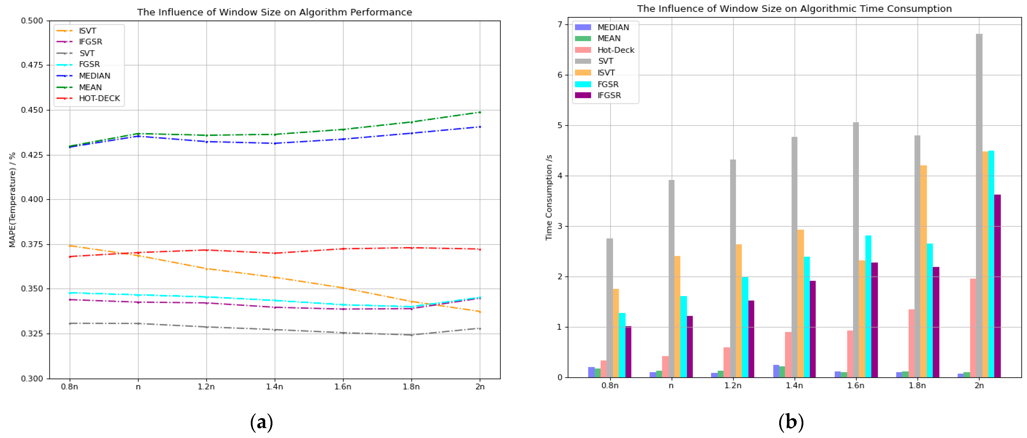
We fix the missing rate of the variable data at 40%, generating missing data randomly. The range for the window size is from 0.8n to 2.0n (where n represents the number of sensors for the current variable, as detailed in Table 1, and the chosen window size is rounded up). We first conduct tests on the temperature data, and Figure 7 presents the results.

As shown in Figure 7a, when we test the temperature data using $MAPE$ as the evaluation standard, the statistical value imputation methods and the hot-deck algorithm exhibit an increase in $MAPE$ with the growing window size. The $MAPE$ of the ISVT algorithm gradually decreases with the increase in the window size. The FGSR, IFGSR, and SVT algorithms have the smallest $MAPE$ when the window size reaches 1.8n. As seen in Figure 7b, the time consumption of the SVT, FGSR, and IFGSR algorithms increases significantly after the window size is 1.8n, and the time consumption of the ISVT algorithm shows little change between the window sizes of 1.8n and 2n. Considering these factors, to achieve higher accuracy and reduce time consumption, we choose 1.8n as the window size for subsequent experiments.

As illustrated in Figure 8a, when we test the pressure data using $MAPE$ as the evaluation standard, the $MAPE$ of the ISVT algorithm and the hot-deck algorithm remains relatively stable. The $MAPE$ values for the FGSR, SVT, and IFGSR algorithms all decrease with an increase in the window size. As seen in Figure 8b, as the time window increases, the time consumption of the hot-deck algorithm and the MCM gradually increases. When the window size is 2n, the time consumption of the IFGSR algorithm is halved compared to the FGSR algorithm and is close to the hot-deck algorithm. For better accuracy, in subsequent experiments, we use 2n as the window size to process data.

As shown in Figure 9a, the $MAPE$ of MCMs exhibits fluctuations with an increase in the window size when different algorithms are applied. The $MAPE$ of ISVT, FGSR, and IFGSR maintains a low level when the window size is 1.6n. The precision of the SVT algorithm remains stable once the window size exceeds 1.6n. As seen in Figure 9b, the time consumption of the MCM does not change much after the window size is 1.4n. Therefore, based on the above results, we select a window size of 1.6n for future experiments on flow rate data.

In summary, through testing on three variables, we have chosen 1.8n as the window size for temperature data, 2n as the window size for pressure data, and 1.6n as the window size for flow rate data for subsequent experiments.

After determining the parameters and the size of the test window, we use the same experimental data to test the performance of various methods under different data loss rates. The evaluation metrics include accuracy and time consumption. The results are as follows.

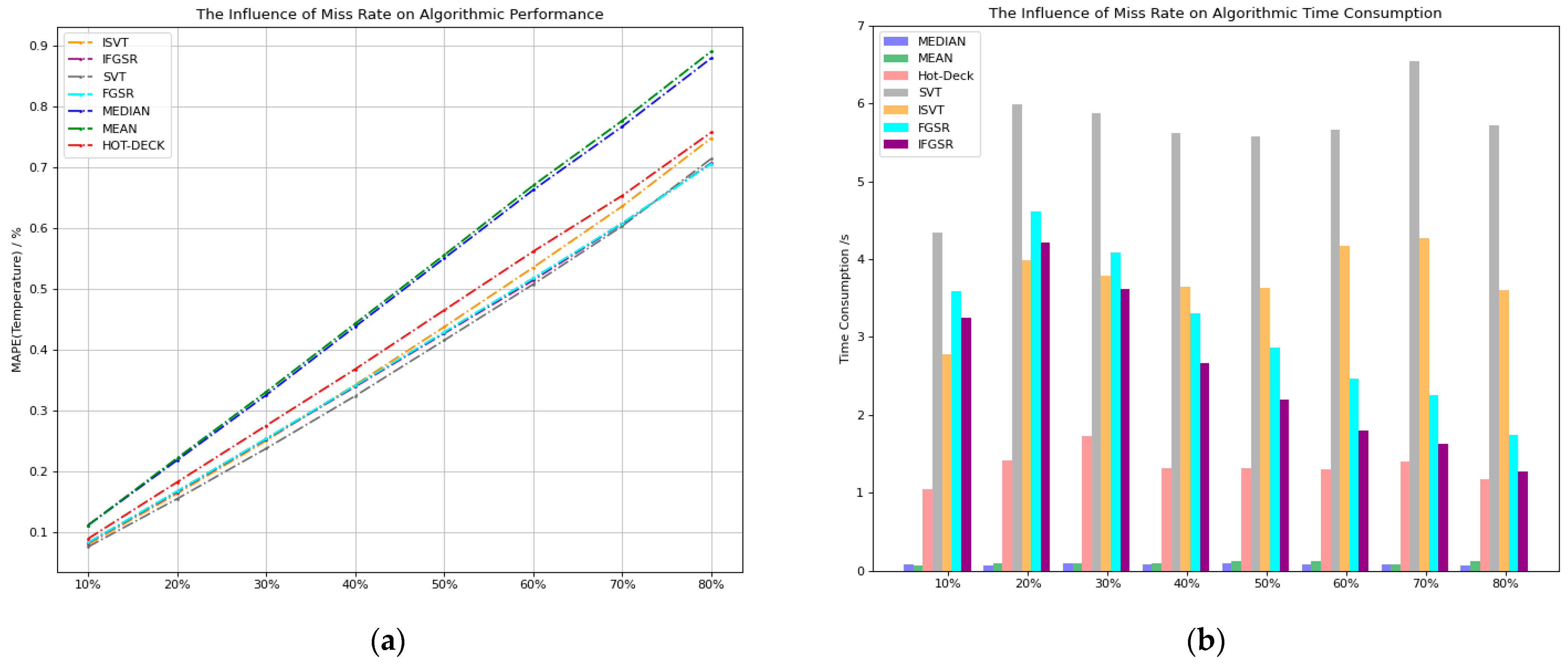
As shown in Figure 10, we first test the temperature data. With a fixed window size, we test the results with a data loss rate of 10% to 80%.

As shown in Figure 10a, when we use $MAPE$ as the evaluation standard, it can be seen that MCMs have the smallest $MAPE$ at any missing rate, ISVT’s $MAPE$ is slightly larger than SVT, and the accuracy performance of IFGSR and FGSR is almost the same. As shown in Figure 10b, the highest time consumption in the MCM is the SVT and FGSR algorithms. In comparison, both ISVT and IFGSR show improvements in time consumption.

In summary, the MCM consistently exhibits the smallest $MAPE$ when processing temperature data. Among them, SVT has the lowest $MAPE$ but the highest time consumption; ISVT’s accuracy is slightly lower than SVT, and the time consumption is lower. The accuracy of FGSR and IFGSR is almost the same, with both slightly underperforming the SVT algorithm. IFGSR has a lower time consumption compared to FGSR, and both significantly reduce time consumption compared to SVT and ISVT.

For pressure data, Figure 11 shows the results of testing data with missing rates ranging from 10% to 80% at a fixed window size.

As shown in Figure 11a, processing pressure data with $MAPE$ as the evaluation metric reveals that FGSR and IFGSR consistently exhibit the smallest $MAPE$. Moreover, the difference in $MAPE$ between IFGSR and FGSR is insignificant across all missing rates. Figure 11b illustrates that the IFGSR algorithm consumes less time than the FGSR algorithm, and its time consumption exceeds only those of the two statistical value imputation methods at high missing rates.

In conclusion, when processing pressure data, the IFGSR algorithm achieves a slight reduction in accuracy compared to the FGSR algorithm but significantly reduces the processing time. Compared to other methods, it also demonstrates higher accuracy and advantages in time consumption.

For flow rate data, Figure 12 shows the results of testing data with missing rates ranging from 10% to 80% at a fixed window size.

Figure 12a illustrates that the MCM exhibits the highest accuracy in processing missing values for flow rate data. The overall accuracy ranking is SVT > FGSR > IFGSR ≈ ISVT. As shown in Figure 12b, considering time consumption, ISVT and IFGSR save a substantial amount of time compared to SVT and FGSR.

In conclusion, when using the MCM to impute the missing values of temperature, pressure, and flow rate data, the SVT, FGSR, and IFGSR algorithms in the MCM consistently demonstrate superior accuracy under any conditions compared to traditional methods, thus validating the applicability of matrix completion for real-time missing data imputation. Furthermore, a comparison between the IFGSR and FGSR algorithms reveals a minor difference in accuracy but a significant reduction in computation time for IFGSR, demonstrating the effectiveness of the improvement method proposed in this paper for matrix completion algorithms used for real-time missing data imputation.

5. Conclusions

This study describes a method for using the MCM to fill in missing values in chemical process data. This method employs matrix completion and sliding windows to process missing data in real-time chemical process data. The fundamental principle involves using the MCM to restore matrices that contain missing values within the chemical process data. In addition, an improvement method is proposed, which enhances the performance of the matrix completion algorithm used for real-time missing data imputation. The results show that the MCM performs well in solving the problem of real-time data missing value imputation in chemical processes, and the proposed improvement method also significantly enhances the computational speed of matrix completion algorithms.

The MCM proposed in this paper does not rely heavily on long-term historical data. It does not need to rely on long-term historical data for detailed modeling of specific devices and then use the model to calculate missing data. It only needs short-term data to obtain relatively accurate results for missing value recovery. This method exhibits good versatility and is applicable to different production devices. The MCM can also predict future data of production devices, and, when combined with appropriate constraints, it can identify and replace outliers.