Load Forecasting and Operation Optimization of Ice-Storage Air Conditioners Based on Improved Deep-Belief Network

Abstract

The prediction of cold load in ice-storage air conditioning systems plays a pivotal role in optimizing air conditioning operations, significantly contributing to the equilibrium of regional electricity supply and demand, mitigating power grid stress, and curtailing energy consumption in power grids. Addressing the issues of minimal correlation between input and output data and the suboptimal prediction accuracy inherent in traditional deep-belief neural-network models, this study introduces an enhanced deep-belief neural-network combination prediction model. This model is refined through an advanced genetic algorithm in conjunction with the “Statistical Products and Services Solution” version 25.0 software, aiming to augment the precision of ice-storage air conditioning load predictions. Initially, the input data undergo processing via the “Statistical Products and Services Solution” software, which facilitates the exclusion of samples exhibiting low coupling. Subsequently, the improved genetic algorithm implements adaptive adjustments to surmount the challenge of random weight parameter initialization prevalent in traditional deep-belief networks. Consequently, an optimized deep-belief neural-network load prediction model, predicated on the enhanced genetic algorithm, is established and subjected to training. Ultimately, the model undergoes simulation validation across three critical dimensions: operational performance, prediction evaluation indices, and operating costs of ice-storage air conditioners. The results indicate that, compared to existing methods for predicting the cooling load of ice-storage air conditioning, the proposed model achieves a prediction accuracy of 96.52%. It also shows an average improvement of 14.12% in computational performance and a 14.32% reduction in model energy consumption. The prediction outcomes align with the actual cooling-load variation patterns. Furthermore, the daily operational cost of ice-storage air conditioning, derived from the predicted cooling-load data, has an error margin of only 2.36%. This contributes to the optimization of ice-storage air conditioning operations.

1. Introduction

Amidst the escalating global emphasis on energy efficiency and sustainable development, myriads of industries confront significant challenges in diminishing energy consumption and enhancing system efficiency [1]. In recent years, the proportion of energy consumed by air conditioning in the total electricity consumption has surged, markedly exacerbating the strain on the power grid due to its substantial electricity usage. Owing to the ability of ice-storage air conditioning systems to store energy during off-peak hours and periods of low electricity prices, these systems can release the stored cold energy during peak load or high electricity price intervals the following day. This assists in “shifting peaks and filling valleys” in air conditioning power consumption, alleviating the burden during peak periods and facilitating the balance between high- and low-demand periods on the power grid. Consequently, this has prompted researchers to delve into the study of ice-storage air conditioning systems [2].

Currently, the prediction of cold load in ice-storage air conditioning systems faces challenges such as low accuracy, delayed responsiveness, and imprecise acquisition of operational parameters, impeding efficient energy management and optimal operation [3]. Accurate cold load forecasting can significantly enhance the management and regulation of ice storage and cooling systems, thereby lowering energy costs and enhancing overall energy efficiency. Moreover, optimizing ice-storage air conditioning involves ensuring a balance between the cooling capacity provided by the chiller and the ice tank during peak and off-peak electricity pricing periods. This process begins with predicting the necessary cold load, followed by allocating cooling capacity based on these predictions [4], Consequently, cold-load prediction is fundamental in optimizing the operation of ice-storage air conditioning systems.

Presently, air-conditioning cooling-load prediction predominantly employs data-driven methods, including Support Vector Machine (SVM), Convolutional Neural Network (CNN), Recurrent Neural Network (RNN), Long Short-Term Memory (LSTM), and Genetic Algorithm (GA) [5]. The LSTM network often experiences a significant decline in generalization ability due to the random initialization of network parameters, making it prone to getting trapped in local optima [6]. SVM, a commonly used artificial intelligence method, is capable of transforming nonlinear relationships but suffers from lengthy data processing times [7]. CNN and RNN models are straightforward and feasible prediction methods, yet their predictive capabilities fall short of SVM [8,9]. However, these relatively common load forecasting methods face issues in several aspects, including the ability to transform nonlinear relationships, data processing time, predictive capabilities, handling time-series and nonlinear data, processing large volumes of complex input data, convergence speed, and accuracy. Additionally, these methods often fail to fully capture the dynamic characteristics and complexity of systems [10]. Deep-belief networks (DBNs) offer a new perspective and tool for a more in-depth analysis and prediction of ice-storage air-conditioning cooling load, demonstrating higher predictive accuracy in scenarios involving high-dimensional, large-scale data load forecasting [11]. Gong et al. [12] (2021) examined traditional load forecasting models in ice storage systems, highlighting the limitations of time-series and regression models and the need for methodological advancements. Yao and Shekhar [13] (2021) explored the efficacy of DBNs in energy demand forecasting within deep learning frameworks, demonstrating their effectiveness in complex data handling and accuracy. However, these studies’ reliance on random initial weights and thresholds in DBNs has led to challenges in ensuring diagnostic accuracy, often resulting in suboptimal prediction due to mismatched input and output data. Addressing these shortcomings in DBN applications thus forms the core focus of this paper.

Meanwhile, several scholars have delved into optimizing the operation of ice-storage air conditioners. Liu et al. [14] (2022) investigated strategies for optimizing ice storage systems, underscoring the significance of scheduling optimization and demand-response strategies in enhancing system efficiency. Gao et al. [15] (2022) identified challenges in applying deep learning models to these systems, specifically concerning data quality, model interpretability, and reliability. While these approaches contribute valuably to the study of ice-storage air-conditioning operation optimization, they often treat load forecasting and operational considerations as distinct entities, overlooking the interdependence of these aspects.

Addressing the aforementioned issues, this study enhances the traditional DBN neural network by integrating the “Statistical Product and Service Solutions” (SPSS) version 25.0 software for data analysis, rather than applying conventional mathematical processing directly to the data. This approach involves conducting a correlation analysis of the system’s input and output variables to increase data interconnectivity. Considering the limitations and characteristics of traditional DBNs, this work combines an improved genetic algorithm (IGA) with the DBN to form a composite prediction model. By employing the IGA to select an optimal set of initial weights and thresholds for the DBN, the approach overcomes the randomness associated with the selection of initial values in traditional DBN models. This strategy enhances the neural network’s capacity for nonlinear generalization and mapping. Compared to the traditional DBN model, the optimized model exhibits faster convergence speed and the ability to escape local optima, offering particular advantages in processing high-dimensional and large-volume data. The IGA-optimized DBN is well-suited for application in research focused on optimizing the operation of ice-storage air conditioning systems, demonstrating its potential to significantly improve performance and efficiency in complex data environments. Experimental results show that the IGA–DBN composite prediction model outperforms common air-conditioning cooling prediction methods, with an average performance improvement of 19.82% and a prediction accuracy of 96.52%. The model demonstrates a more significant prediction discrepancy with larger data volumes and an average increase in convergence speed of 22.36%. Moreover, the daily operational cost error for ice-storage air conditioning, derived from the predicted cooling-load data, is only 2.56%, facilitating the further optimization of such air conditioning systems.

2. Ice-Storage Air Conditioning Cold-Load Prediction and Operation Optimization Process

The primary challenge in predicting the cold load of ice-storage air conditioning systems lies in enhancing accuracy and timeliness. Traditional methods have not effectively integrated cold-load prediction with the operational dynamics of these systems. Therefore, it is crucial to re-analyze and re-integrate data based on real-world application scenarios for more effective guidance in optimizing the operation of ice-storage air conditioning.

The cold-load prediction and operation optimization process of the ice-storage air conditioner in this paper is shown in Figure 1. The initial step involves utilizing SPSS version 25.0 software data analysis software to perform a correlation analysis on the input data for the cooling load of ice-storage air conditioning. This includes conducting Pearson correlation significance tests to enhance the interconnectedness of the data, allowing for the exclusion of four variables with the least strongest correlations: solar radiation intensity at time t, solar radiation intensity at time t − 1, wind speed at time t, and atmospheric pressure at time t. This process selects six variables as input for the IGA–DBN neural-network prediction model: outdoor dry-bulb temperature at time t − 1, outdoor dry-bulb temperature at time t, cooling load at time t − 1, cooling load at time t − 2, cooling load at time t − 3, and relative humidity at time t. This selection aims to address the limitations caused by low correlations between input and output variables, such as slow network training speed and low prediction accuracy, thereby improving the model’s predictive accuracy. Furthermore, addressing the traditional GA’s drawbacks, such as slow search speed and premature convergence, and its fixed crossover and mutation probabilities based on experience, which are unsuitable for different function optimization problems, improvements to the GA are proposed. Subsequently, the IGA is used to select an optimal set of initial weights and thresholds for the DBN, overcoming the randomness in the selection of initial values. This enables the DBN to achieve faster convergence speed and the ability to escape local optima while leveraging the neural network’s nonlinear generalization and mapping capabilities, resulting in the IGA–DBN composite prediction model. This model is then applied to the prediction of the cooling load for ice-storage air conditioning. To demonstrate the superiority of the improved model, this study calculates and analyzes the operational costs of two typical air conditioning operational modes—ice-storage priority operation mode and unit priority operation mode—using the air-conditioning cooling-load prediction results from the composite prediction model.

3. Analysis of the Working Principle and Operation Mode of Ice-Storage Air Conditioner

3.1. Working Principle of Ice-Storage Air Conditioning

The ice-storage air conditioning system consists of refrigeration units, ice storage devices, connecting pipes, and control regulators, among other equipment, and is primarily divided into four main systems: the source of cold system, chilled water system, cooling water system, and control system. The source of cold system is a key component that distinguishes the ice-storage air conditioning system from conventional air conditioning systems. It is composed of dual-mode refrigeration units and ice storage devices. The chilled water system uses water as the cooling medium and includes chilled water pumps, air conditioning terminals, and chilled water pipelines. The cooling water system also uses water as the cooling medium and comprises refrigeration units, cooling water pumps, pipelines, and cooling towers. The control system is made up of communication systems, sensors, controls, and actuators. It forms the foundation for the economical and energy-saving operation of the ice-storage air conditioning system. In addition to the start–stop control of system electromechanical equipment, the control system also integrates peak–valley electricity prices and the next day’s cooling-load demand. It controls and adjusts the working state of the refrigeration units’ ice-making condition, the distribution of cooling capacity between the refrigeration unit in the cooling condition and the ice storage device, and the working state of the refrigeration unit in the cooling condition. This achieves economic and energy-saving benefits.

In ice-storage air conditioning systems, understanding the components and behaviors of cold load is crucial when leveraging low electricity prices. In this study, the cold load composition primarily consists of indoor and outdoor heat loads, encompassing factors such as ventilation rates, building structures, electrical equipment, solar radiation, and external temperatures. Addressing these components, ice-storage air conditioning systems often employ advanced intelligent control systems to adjust based on factors like indoor and outdoor temperatures, building loads, and electricity prices, aiming to minimize power consumption while ensuring comfort. Through effective load management, such as adjusting indoor temperatures and optimizing building insulation, overall cold load is reduced. The efficient cycling of ice storage and energy storage is employed to meet cold load demands and utilize low electricity prices effectively. The operation of ice-storage air conditioning systems is closely intertwined with efficient cycling of ice storage and energy storage. Ice-storage air conditioners operate on a diurnal cycle, encompassing night-time ice storage and daytime cooling. The ice storage phase predominantly occurs during off-peak hours in the power grid, where the air conditioning system utilizes phase-change latent heat for ice formation, typically employing direct electricity for ice storage. During the daytime, when end-users require cooling, the system enters the cold supply phase. This period coincides with peak demand for cooling load and higher electricity prices. The operation of refrigeration units and ice storage equipment during this time allows for joint cold supply from the chiller and ice tank. This strategy facilitates “shifting peaks to fill valleys” in electricity usage, alleviating grid pressure during peak periods and enhancing demand-response flexibility [16]. An ice-storage air conditioning schematic diagram is shown in Figure 2.

3.2. Mode of Operation of Ice-Storage Air Conditioners

The advantages of ice-storage air conditioning systems encompass two main aspects. Firstly, they can facilitate peak shifting in the power grid, effectively balancing the load by storing cooling energy during off-peak hours (“valley”) and utilizing it during peak hours (“peak”). Secondly, by leveraging time-of-use electricity pricing policies that differentiate between peak, off-peak, and mid-peak (or “flat”) rates, these systems can significantly reduce the operational costs of air conditioning. The extent to which an ice-storage air conditioning system can maximize its advantages is not only dependent on the rationality of its design but also on the appropriateness of its operational mode. An operational mode of an ice-storage air conditioning system refers to the strategy applied over a cycle of operation that aligns with the next day’s hourly cooling-load demand. This strategy plans the amount of ice to be stored during the ice-making phase and distributes the load between the refrigeration units and the ice storage device during the cooling phase, in accordance with the structure of electricity tariffs. Therefore, optimizing the operation of ice-storage air conditioning systems by utilizing time-of-use electricity rates can effectively lower their operational costs. This optimization involves planning the ice production and storage for periods when electricity is cheaper and using the stored ice for cooling during periods when electricity prices are higher, thus achieving economic and energy-saving benefits.

The optimization of ice-storage air conditioner operation involves identifying the optimal point for switching between various modes to maximize energy savings and reduce consumption. Advanced prediction of cold load is critical for determining the operation mode of these air conditioners and for the efficient control of the main engine in conjunction with the ice tank. Ideally, the chiller operates minimally during peak electricity consumption periods to minimize operational costs. This paper’s research emphasizes the method for predicting the cold load of ice-storage air conditioners and its role in guiding operational optimization. Consequently, the study utilizes the enhanced DBN combination prediction model to analyze two prevalent operation modes: ice-storage priority and unit priority. The effectiveness of the proposed prediction method is demonstrated through the calculation of operational costs under these modes.

In ice-storage priority mode, the air conditioner initially uses a cooling tower and ice unit to produce ice at night, storing it in an ice bank. During the day, the stored ice is the primary source for meeting cooling demands. When the ice supply is insufficient, the refrigeration unit supplements the necessary cooling capacity. This mode’s primary advantage is maximizing electricity usage during low-tariff hours, thus conserving energy and reducing operating costs. Conversely, in unit priority mode, the refrigeration unit primarily addresses the immediate cooling demand. The ice storage is utilized either when the refrigeration unit’s capacity is insufficient or to optimize operating costs. Typically employed outside peak daytime tariff hours or when immediate response to significant cooling demands is necessary, this mode offers more flexible control and quicker response times, although it may not be as energy-efficient as the ice-storage priority mode [17].

4. Improved DBN Ice-Storage Air Conditioner Prediction Modeling

4.1. The DBN Model

Deep-belief networks are multilayered probabilistic generative models extensively utilized in feature learning and classification of intricate datasets. DBNs effectively amalgamate the characteristics of neural networks with probabilistic graphical models, enabling them to proficiently process nonlinear and high-dimensional data. As generative models, DBNs distinguish themselves by learning the joint distribution of the provided data—a capability that extends beyond mere classification to the generation of new data samples. 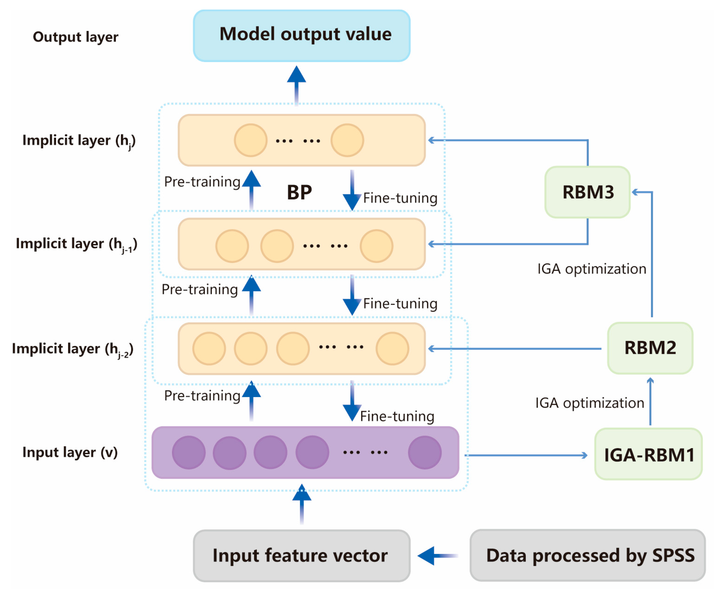The architecture of a DBN comprises multiple hidden layers, with each layer responsible for learning distinct features and representations of the data [18]. This layered, hierarchical approach renders DBNs particularly adept at extracting features from complex data structures. The structural configuration of DBNs is depicted in Figure 3.

The training process of DBNs is a well-designed multi-step process that aims to maximize the capture and characterization of the input data. This process can be divided into two main parts: layer-by-layer pre-training and global fine-tuning.

In the context of layer-by-layer pre-training within a DBN, the architecture comprises multiple layers of Restricted Boltzmann Machines (RBMs), each tasked with capturing features from various levels of input data. During this pre-training phase, each RBM layer is trained independently, without the influence of other layers. This independence allows each layer to concentrate solely on learning feature representations from its received input, beginning from the bottom layer and ascending sequentially through the DBN hierarchy [19]. Successive layers of RBMs utilize the output from the preceding layer as their input. Consequently, the RBMs in the lower layers of the network are adept at learning fundamental data features, while those in the higher layers progressively extract more abstract and complex feature representations. The corresponding calculation is shown in Equation (1):

$$\begin{array}{c}{h}_j=w_{ij}{v}_i+b_j\\ v_i=w_{ij}{h}_j+a_i\end{array}$$

(1)

where $v_i$, $a_i$ are the i-th neuron input and bias of the visible layer; $h_j$, $b_j$ are the j-th neuron output and bias of the hidden layer; and $w_{ij}$ is the connection weight between the neurons of the visible and hidden layers.

The visible layer probability distribution function $E(\nu ,h)$ for each layer in the RBM network is defined as shown in Equation (2):

$$E(\nu ,h)=-\sum _{i=1}^n{a}_i{\nu }_i-\sum _{j=1}^m{b}_j{h}_j-\sum _{i=1}^h\sum _{j=1}^m{\nu }_j{w}_{ij}{h}_j$$

(2)

where $h$, $m$ are the number of neurons in the visible and hidden layers, respectively.

The probability distribution function $P(v)$ of the visible layer of each RBM network is defined as shown in Equation (3):

$$P(v)=\frac{{\displaystyle \sum _h}{\mathrm{e}}^{-E(v,h)}}{{\displaystyle \sum _{\nu ,h}}{\mathrm{e}}^{-E(\nu ,h)}}$$

(3)

Given the independence of neurons within the same layer, it is possible to calculate the probability associated with the weight $v_i=1$ as follows:

$$P(v_i=1|h)=\mathrm{Sigmoid}(a_i+{\displaystyle \sum _{i=1}^m{h}_j}{w}_{ij})$$

(4)

Similarly, the probability associated with the activation function $h_j=1$ can be calculated:

$$P(h_j=1|v)=\mathrm{Sigmoid}(b_j+{\displaystyle \sum _{i=1}^n{v}_i}{w}_{ij})$$

(5)

$\mathrm{Sigmoid}\left(\right)$ function is referred to as the activation function in the context of neural networks:

$$\mathrm{Sigmoid}(x)=\frac{1}{1+\exp (-x)}$$

(6)

The primary objective of RBM pre-training is to initially obtain optimal parameters, denoted as parameter $\theta$, represented by ${\theta }^{*}$, to achieve a DBN structure with a satisfactory fitting effect. At this stage, the sample statistical probability within the DBN and the model-generated probability are maximized to be equal. The calculation formula for ${\theta }^{*}$ is as follows:

$${\theta }^{*}=\mathrm{argmax}{\displaystyle \sum _{t=1}^T\mathrm{Inp}}(v^t)$$

(7)

where T denotes the total number of training samples.

Global fine-tuning entails the comprehensive refinement of a DBN using the Back Propagation (BP) algorithm, following the pre-training of all layers. This phase aims to adjust the weights and biases across the network, enabling improved data representation and prediction. Utilizing the error gradient, the BP algorithm methodically updates the parameters from the top layer downwards, thereby enhancing the network’s predictive capabilities [20]. The significance of the fine-tuning phase lies in its integration of individual layer learnings, ensuring the DBN’s collective and effective representation of the data. After pre-training, the DBN acquires initial parameters. The fine-tuning phase aims to enhance the model’s fitting performance. Starting from the topmost layer of the DBN, fine-tuning adjusts the initial parameters layer by layer downwards using a small amount of labeled data obtained during pre-training. Typically, the SoftMax function is employed as the final classifier, with the BP algorithm used to execute the fine-tuning process. If the DBN network comprises l RBMs, the output of the pre-training is as follows:

$$u^l(x)=\mathrm{Sigmoid}(a^l+w^l{u}^{l-1}(x))$$

(8)

The SoftMax function determines the output of the DBN by identifying the category with the highest probability as the predicted class. This process effectively translates the network’s output into a probability distribution over predicted classes, facilitating classification tasks by emphasizing the most likely category.

In the initialization phase of the DBN architecture, a DBN model is established. Traditionally, the selection of optimal initial weights and thresholds in DBN models is randomized, which closely ties the iteration time to network parameters and adversely affects the global search capability. To address this issue, this study proposes the use of an improved GA to optimize the DBN, thereby overcoming the randomness in the selection of initial DBN weights and thresholds. This approach continuously guides the optimization of DBN parameters during model training, enhancing the model’s learning efficiency and predictive accuracy [21].

4.2. IGA–DBN Neural-Network Prediction Model

In the exploration of ice-storage air conditioning systems, the pivotal roles of load forecasting and operational optimization are underscored by their contributions to enhancing energy efficiency and curbing operational expenses. The DBN emerges as the preferred analytical instrument, selected for its exemplary prowess in feature extraction and data modeling. This study leverages the DBN’s predictive insights, in concert with findings from an optimization algorithm, to refine the operational parameters of ice-storage air conditioners. Central to the predictive model architecture, the paper examines the learning efficacy of the RBM using reconstruction error (RE). Predominantly utilized in machine learning and signal processing, the RE evaluates the disparity between original and reconstructed data, serving crucially in dimensionality reduction and feature extraction tasks table. An incremental approach, adding RBM layers successively, facilitates the observation of RE variations. Notably, a diminished RE is indicative of more comprehensive feature extraction and enhanced model stability, as elaborated in Equation (9). The experiment sets the maximum number of iterations of the network model to 100, the learning rate is $\gamma =0.01$, and the learning increase coefficient and learning decrease coefficient are $\mathrm{IN}=1.14$ and $\mathrm{DE}=0.86$.

$$\mathrm{RE}(t)=\sum _{k=1}^N{(X_k-{\nu }_t)}^2$$

(9)

where $\mathrm{RE}(t)$ is the reconstruction error value of the t-th iteration, $N$ is the number of samples, $X_k$ is the k-th column of the input sample matrix, and ${\nu }_t$ is the current input layer neuron state.

The iterative analysis reveals a consistent downward trend in the reconstruction error (RE) values across the various layers of the RBM. Notably, there is a gradual decline in RE as the depth of the model increases. Each subsequent RBM layer initially presents a larger RE, surpassing the final value of its preceding layer, attributed to the random assignment of initial weights. This dynamic is further elucidated in

Table 1. Effect of DBN depth on RE.

Network Depths	RE	Computation Time/s
1-layer RBM	0.6772~2.2865	82.3
2-layer RBM	0.0431~0.9426	115.2
3-layer RBM	0.0397~0.7686	141.5
4-layer RBM	0.0343~0.6214	189.6

, which illustrates the impact of the DBN model depth on the RE. Table 1 indicates a progressive decrease in network reconstruction error with increasing depth. However, this is accompanied by rising computational time and diminished efficiency. Specifically, a single-layer RBM network exhibits substantial fluctuations in RE and slower convergence. In contrast, a two-layer RBM network demonstrates a decreasing RE trend with quicker convergence. While the arithmetic time for three-layer and four-layer RBM networks is more complex, the four-layer network does not show significant improvements in steady-state error value or convergence speed compared to the three-layer network. Consequently, this study opts for a three-layer RBM architecture for the cold-load DBN prediction model.

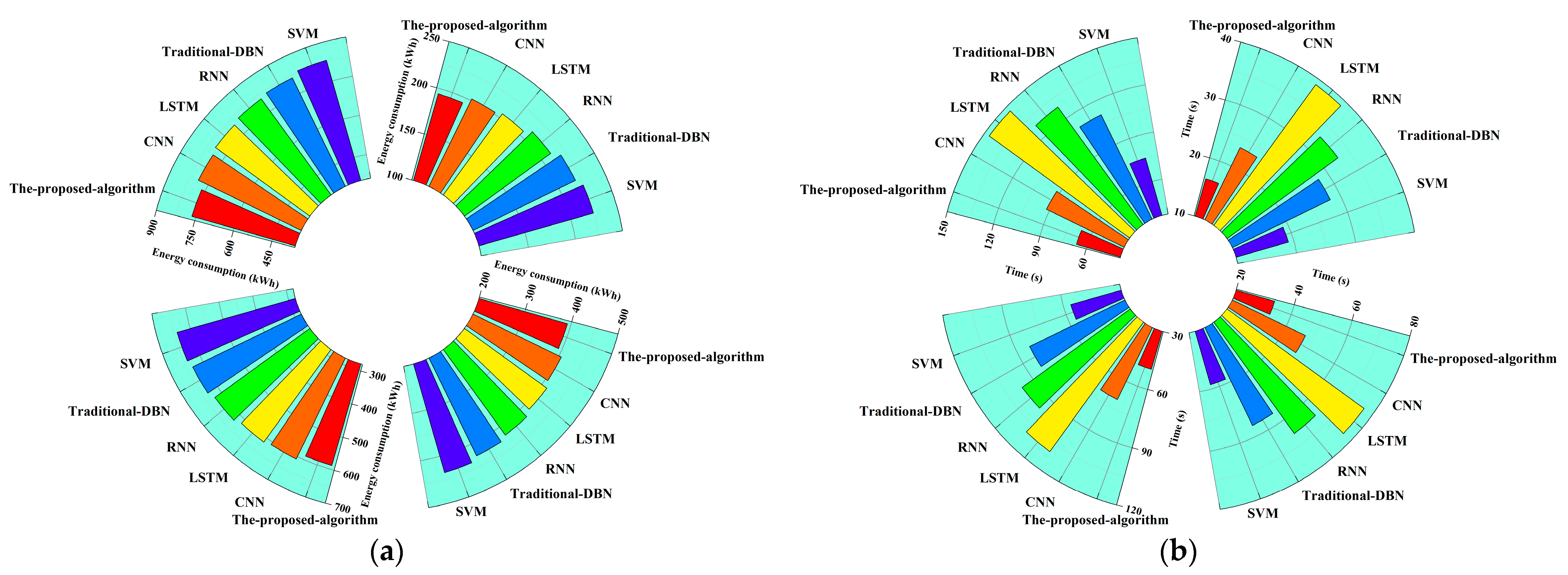
Simultaneously, to demonstrate the advantages of the DBN in tasks such as dimensionality reduction and feature extraction compared to other traditional network models, this study benchmarks against the computational time taken for reconstructing errors with three layers of the RBM in a traditional DBN network. It also involves training and calculating the computational times of conventional networks, including CNN, RNN, SVM, and LSTM networks. The specific outcomes are presented in

Table 2. Computation time of each neural network regarding RE.

Network Model	RE	Computation Time/s
DBN	0.0397~0.7686	141.5
LSTM	0.0419~0.7881	155.2
RNN	0.0423~0.7897	161.5
CNN	0.0421~0.7799	169.6
SVM	0.0425~0.7673	171.2

.

When the training conditions for the model remain unchanged, and after training different layers of CNN, RNN, SVM, and LSTM networks to meet a steady-state error and convergence speed within the RE range of 0.0397 to 0.7686, it was found that compared to the DBN model, the computational time for these four types of network models increased to a certain extent, with the maximum increase in computational duration reaching 17.35%. This demonstrates that the DBN model possesses superior convergence capabilities compared to other traditional network models, offering significant advantages in tasks such as high-dimensional data computation and feature extraction.

Having established the optimal depth for the RBM in the DBN prediction model, this study next addresses a fundamental challenge in traditional DBN models: the arbitrary selection of initial weights and thresholds. To rectify this, the research introduces an optimization of the DBN model using the improved IGA, specifically designed to reduce the randomness in selecting initial DBN parameters [22]. The traditional GA employs binary coding, representing individuals within the population with fixed-length binary strings, where alleles are comprised of binary symbols from the set {0,1}. The selection process utilizes the roulette wheel selection method; for crossover, single-point crossover is used with a fixed crossover probability; and mutation is carried out through bit mutation, with mutation probability also set to a fixed value. In this study, four operational parameters of the basic GA need to be predetermined: the population size M, which refers to the number of individuals within the population, is set to 100; the termination criterion for genetic operations G is set to 500 generations; the crossover probability P_c is set within the range of (0.4, 0.9); and the mutation probability P_m is set within the range of (0, 0.1). However, traditional GAs exhibit drawbacks such as slow search speed and a tendency towards premature convergence. Moreover, the fixed values for crossover probability P_c and mutation probability P_m, based on experience, may not be suitable for different function optimization problems. However, traditional GAs suffer from limitations such as slow search speeds and a propensity for premature convergence. Furthermore, the conventional approach of using fixed values for crossover probability (P_c) and mutation probability (P_m), based on empirical judgment, limits their applicability across diverse optimization problems. In response, this paper proposes modifications to the GA, particularly in the adaptation of P_c and P_m during the evolutionary process [23]. The traditional adaptive genetic algorithm (AGA), which dynamically adjusts crossover and mutation probabilities (P_c and P_m, respectively) based on fitness values, allows these probabilities to automatically change with fitness. However, when the fitness values of individuals are close to or equal to the maximum fitness value, both P_c and P_m approach zero. This condition is detrimental in the early stages of evolution, as superior individuals nearly remain unchanged, increasing the likelihood of converging to local optima.

Considering the limitations of traditional AGAs, where the crossover and mutation probabilities become zero when the fitness value equals the maximum fitness value, there is a tendency to converge to local optima. Additionally, individuals with lower fitness exhibit reduced mutation capabilities, leading to stagnation. While the elitist strategy protects the optimal individuals, it may cause the population’s evolution to stall when the number of individuals is large, leading to local convergence. Furthermore, traditional adaptive GAs have focused solely on the comparison between the average and optimal values within the population, neglecting a comprehensive evaluation of how crossover and mutation probabilities are set across the entire population. The modified approach allows P_c and P_m to dynamically regulate the algorithm’s search efficiency without compromise. These probabilities are crucial in influencing the GA’s behavior and performance. To escape local optima, P_c and P_m are increased when the population’s fitness con-verges towards a local optimum. Conversely, if the population’s fitness is more varied, P_c and P_m are reduced to preserve superior individuals. Additionally, individuals with fitness levels above the population average are assigned lower P_c and P_m to facilitate their progression to subsequent generations, while those below the average are subjected to higher P_c and P_m values to facilitate their elimination. Based on the adaptive genetic algorithm, the variation in crossover and mutation probabilities follows a specific rule: individuals of lower fitness are assigned higher crossover probabilities and lower mutation probabilities. Conversely, individuals of higher quality are allocated crossover and mutation probabilities based on their fitness level and the iteration state. As the number of iterations approaches the maximum, the crossover probability decreases, while the mutation probability increases. The improved adaptive genetic algorithm automatically adjusts the crossover and mutation probabilities, as shown in Equations (10) and (11).

In order to further improve the accuracy of the prediction model, the best initial weights and threshold parameter configurations of the DBN model are optimized using the IGA in this paper as follows:

Step 1: Initialize the parameters in the DBN network, select the number of neuron layers and the number of neurons in the DBN, and then select the dimensions of the individuals to establish the DBN network structure.

Step 2: Initialize the GA population to produce N individuals constituting the initial solution set. Encoding the initial values of the DBN model by an improved GA.

Step 3: Determine the fitness function $f=1/ob$, and calculate the fitness $f_j$.

Step 4: Individuals are selected according to roulette rules, and the average fitness value of the current population, $f_{avg}$, and the maximum fitness value of the current population, $f_{max}$, are calculated.

Step 5: Individuals in the population are randomly paired into pairs, and their crossover probability P_c is calculated by the adaptive crossover formula, which randomly generates $R(0,1)$, and the crossover operation is performed on the chromosome if $R<P_c$. The adaptive crossover probability formula is shown in Equation (10):

$$P_c=\left\{\begin{array}{c}\left\{\frac{k_1(f_{max}-f^{\prime })}{f_{max}-f_{a\nu g}},f^{\prime }>f_{a\nu g}\right.\\ k_2,f^{\prime }\le f_{a\nu g}\end{array}\right.$$

(10)

where $f_{a\nu g}$ denotes the average fitness value of the current population, $f_{max}$ denotes the maximum fitness value of the current population, $f^{\prime }$ denotes the fitness value of the i-th chromosome, and $k_1$, $k_2$ are set parameters.

Step 6: For all individuals in the population, their adaptive mutation probability P_m is calculated by the adaptive mutation formula, $R(0,1)$ is randomly generated, and crossover operation is performed on the chromosome if $R<P_m$. The adaptive mutation probability adjustment formula is shown in Equation (11):

$$P_m=\left\{\begin{array}{c}\left\{\frac{k_3(f_{\max }-f)}{f_{\max }-f_{a\nu g}},f>f_{a\nu g}\right.\\ k_4,f\le f_{a\nu g}\end{array}\right.$$

(11)

where $f_{a\nu g}$ denotes the average fitness value of the current population, $f_{\max }$ denotes the maximum fitness value of the current population, $f$ denotes the fitness value of the i-th chromosome, and $k_3$, $k_4$ are set parameters.

Step 7: The fitness of new individuals generated from crossover and mutation is calculated. Low-fitness individuals generate new individuals after being manipulated by the IGA algorithm, and the resulting population of new individuals is mixed with the good population to form a new population.

Step 8: At the end of evolution, determine whether the accuracy meets the requirements, select the best fitness value, i.e., the optimal weight threshold, and then assign the optimized weight threshold to the DBN; otherwise, return to step 4 to continue training.

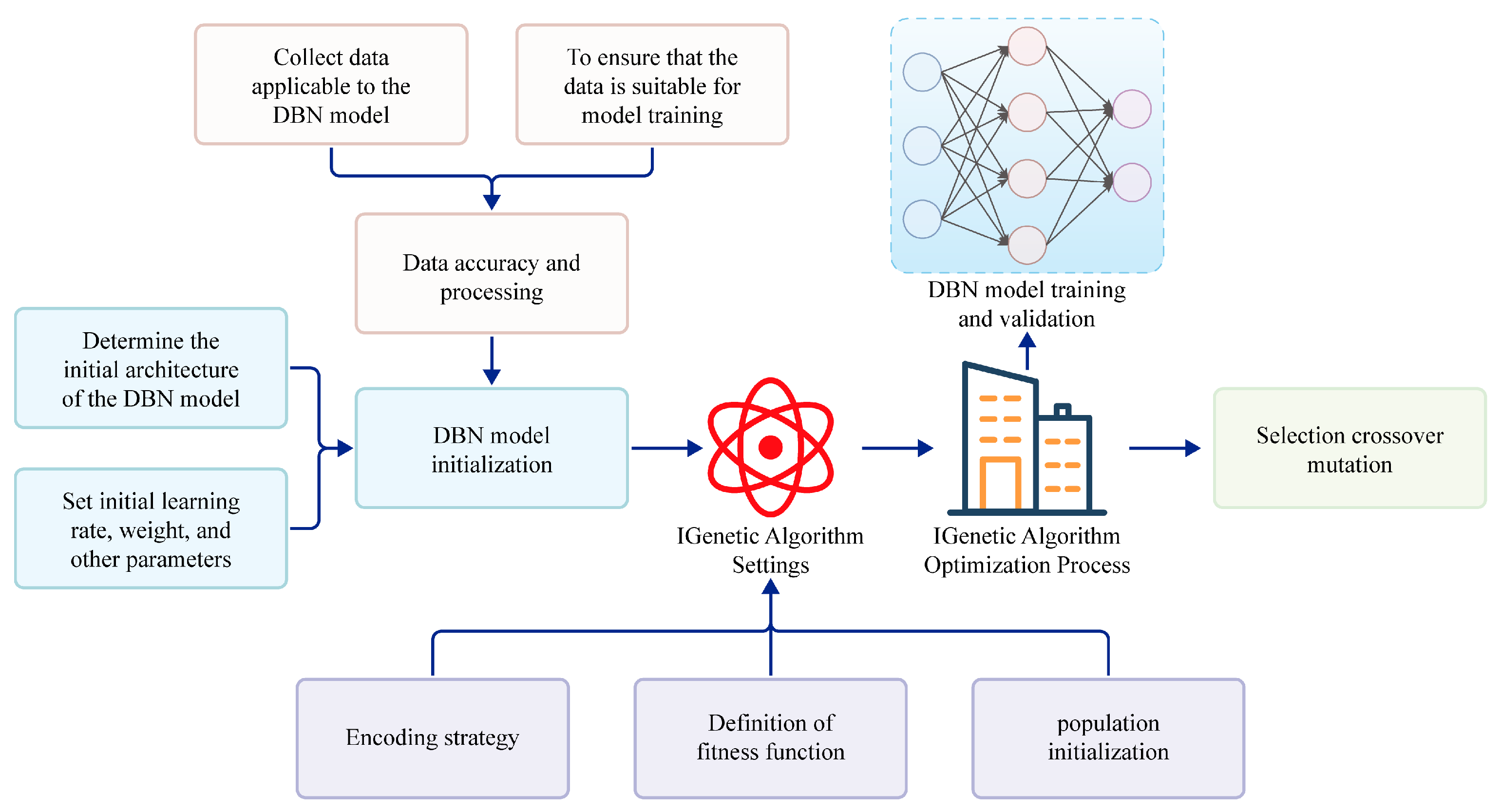
The architecture of the DBN prediction model, enhanced through the use of the IGA, is depicted in Figure 4. This architecture represents an iterative process, where the IGA–DBN model achieves adaptive adjustments. These adjustments are facilitated by refining the P_c and P_m within the GA and integrating it with the DBN, renowned for its superior feature extraction capabilities. The IGA’s primary role in this framework is to address the issue of random initialization inherent in DBN weight parameters. It continually optimizes the parameters of the DBN, and the performance feedback from the DBN model informs subsequent rounds of IGA-guided parameter optimization. This synergistic combination of the IGA with the DBN model significantly enhances the latter’s efficacy in handling complex data processing tasks.

4.3. Load Forecast Evaluation Indicators

In order to better measure the prediction effect of the IGA–DBN prediction model, this paper utilizes three evaluation indexes to evaluate it, including Mean Absolute Error (MAE), Root-Mean-Square Error (RMSE) and Mean Relative Percentage Error (MAPE). The specific expressions are shown in Equations (12)–(14):

$$\mathrm{MAE}=\frac{1}{N}\sum _{t=1}^N|y_i-y_a|$$

(12)

$$\mathrm{RMSE}=\sqrt{\frac{1}{N}\sum _{t=1}^N{(y_i-y_a)}^2}$$

(13)

$$\mathrm{MAPE}=\frac{1}{n}\sum _{i=1}^N\left|\frac{y_i-y_a}{y_i}\right|\times 100\%$$

(14)

where $N$ denotes the total number of selected samples, $y_i$ denotes the actual value of electricity load, and $y_a$ denotes the predicted value.

5. Example Analysis

5.1. Data Processing

To validate the proposed method, this study utilizes some data from the 2017 UCI Machine Learning Repository’s energy prediction dataset, encompassing around 145 days of recordings at 10 min intervals [24]. In applying the IGA–DBN neural network, the study confronts challenges related to the redundancy of input data and biases in combined prediction, which complicates achieving optimal prediction accuracy in practical engineering scenarios. A significant aspect of this research involves addressing the low correlation between certain input and output datasets. To enhance the correlation strength, a thorough analysis using SPSS software is conducted, emphasizing the significance of the Pearson correlation coefficient. This process aims to augment data correlation and discard input variables with minimal correlation. Such an approach is designed to compensate for the shortcomings of traditional prediction methods, which often suffer from prolonged neural-network training times and diminished prediction accuracy due to low correlations between input and output variables. Consequently, these measures are expected to substantially improve the accuracy of the IGA–DBN model [25]. For training the IGA–DBN neural network, this study utilized input data comprising 24 h periods across the first 50 days of a 60-day span in July and August. The data from 25 to 30 August were designated validation analysis data. The selection of model input variables was informed by the Pearson correlation coefficient analysis, as detailed in

Table 3. Correlation between input impact factors and cooling load at time t.

Input Variable	Correlation Coefficient	Input Variable	Correlation Coefficient
outdoor dry-bulb temperature at time t − 1	0.7789	solar radiation intensity at time t	0.4914
outdoor dry-bulb temperature at time t	0.7674	relative humidity at time t	0.7097
cold load at time t − 1	0.9585	cold load at time t − 2	0.8197
intensity of solar radiation at time t − 1	0.4345	cold load at time t − 3	0.7113
wind velocity at time t	0.0647	air pressure at time t	0.0245

. This analysis categorized correlation strengths into four ranges: weak ([0, 0.3]), medium ([0.3, 0.5]), strong ([0.5, 0.7]), and very strong ([0.7, 1.0]). To enhance data stability and processing efficiency, variables within the [0.7, 1.0] range, indicating a very strong correlation, were chosen for the simulation analysis. Post-correlation analysis, as outlined in Table 3, four variables were excluded due to weaker correlations: solar radiation intensity at time t and t − 1, wind speed at time t, and barometric pressure at time t. Consequently, six variables demonstrated sufficient correlation for inclusion as input parameters: outdoor dry-bulb temperature at times t − 1 and t, cooling load at times t − 1, t − 2, and t − 3, and relative humidity at time t. These variables, demonstrating robust correlation, were integrated into the IGA–DBN neural network, with the cold load at time t serving as the output variable.

In addition, since the input data are not of the same order of magnitude, this paper uses Equation (15) deviation normalization to normalize the input data. The model output values are back-normalized by Equation (16) to obtain the actual predicted values.

$$x_i^{\prime }=\frac{(x_i-x_{min})}{(x_{max}-x_{min})}$$

(15)

$$y_i=y_{min}+o_i(y_{max}-y_{min})$$

(16)

where $x_i$ is the original value of sample; $x_{min}$ is the original sample minimum; $x_{max}$ is the original sample maximum; $x_i^{\prime }$ is the normalized processing value; $o_i$ is the output value, $y_{min}$ is the output minimum, $y_{max}$ is the output maximum, and $y_i$ is the output reduced value.

5.2. IGA–DBN Predictive Model Validation Analysis

The implicit layers of the DBN network, the number of nodes in each layer, and the settings of the relevant parameters play a crucial role in the effectiveness of the model prediction. In this paper, a three-layer implicit layer design is used, and the total number of layers in the network is five, with six input layer nodes and one output layer node. The number of implicit layer nodes is determined according to Equation (17):

$$N_h=\frac{N_S}{\alpha \times (N_i+N_o)}$$

(17)

where $N_i$ is the number of neurons in the input layer; $N_o$ is the number of neurons in the output layer; $N_S$ is the number of samples in the training set; and $\alpha$ is an arbitrary constant value that can be self-taken in [2,3,4,5,6,7,8,9,10]. Using a single RBM interval training test, the DBN network structure can be obtained as 6-15-10-10-1. Its parameter settings are shown in

Table 4. Configuration of IGA–DBN prediction model parameters.

Parameters	Configuration	Parameters	Configuration
network layers	5 layers	DBN momentum	0.9
DBN learning rate	0.01	batch-size	50
weight decay	0.0001	iterations	100

.

Following the established model parameter configurations and the elimination of low-correlation input data using SPSS, this study conducts predictions using test data across six experimental models. These models include the traditional DBN model, CNN, RNN, SVM, LSTM, and the method proposed in this paper. A detailed comparison of the prediction results obtained from these models is presented in Figure 5.

To demonstrate the superiority of the IGA-optimized DBN model over other predictive models, this study establishes six experimental groups, encompassing traditional DBN models, CNN, RNN, SVM, LSTM, and the methodology proposed in this paper. Comparative analyses are conducted under uniform parameter settings, focusing on several key aspects. These include prediction performance metrics such as accuracy, recall, precision, and F1Score, as well as the model’s energy consumption and operational efficiency. Additionally, load prediction evaluation metrics, namely MAE, RMSE, and MAPE, are also assessed to provide a comprehensive evaluation of each model’s effectiveness.

5.2.1. Comparative Analysis of Predicted Performance

The performance metrics of the load forecasting model include accuracy, recall, precision and F1Score. The specific calculations are shown in Equations (18)–(21):

$$\mathrm{Accuracy}=\frac{TP+TN}{TP+FN+TN+FP}$$

(18)

$$\mathrm{Recall}=\frac{TP}{TP+FN}$$

(19)

$$\mathrm{Precision}=\frac{TP}{TP+FP}$$

(20)

$$\mathrm{F}1\mathrm{Score}=(1+{\beta }^2)\times \frac{\mathrm{Precision}\times \mathrm{Recall}}{({\beta }^2\times \mathrm{Precision})+\mathrm{Recall}}$$

(21)

where $TP$ (True-Positive), indicates that the positive class is predicted to be positive; $TN$ (True-Negative), indicates that the negative sample is predicted to be negative; $FP$ (False-Positive), indicates that the negative class is predicted to be positive; and $FN$ (False-Negative), indicates that the positive class is predicted to be negative.

As illustrated in Figure 6, the optimized DBN model demonstrates the highest accuracy across all data volumes, reaching a prediction accuracy of 0.9652 when the data volume is 200. This indicates that the optimization strategy effectively enhances the model’s predictive performance. Compared to traditional DBN, CNN, RNN, LSTM, and SVM models, the optimized DBN exhibits superior performance at all data levels, particularly showing significant improvements over the traditional DBN model. In terms of recall, the optimized DBN model achieves the highest recall rates across all data levels, indicating that the optimization strategy effectively improves the model’s ability to identify positive samples. Compared to traditional models of the same category, the optimized DBN model has a stronger advantage in recall, especially when dealing with large datasets. For instance, the recall rate of the optimized model reaches 0.9257 when the data volume is 200. Regarding precision, the accuracy of all models increases with the volume of data, reflecting the positive impact of increasing training data volume on enhancing model performance. The precision of the optimized DBN outperforms other models, including traditional DBN, CNN, RNN, LSTM, and SVM, benefiting from its advanced feature extraction capabilities and the incorporation of a GA. When the data volume is 200, the precision of the optimized model also reaches 0.9486. From the perspective of the F1Score, the optimized model shows superior performance in both precision and recall, ensuring balanced and efficient performance. Compared to other models, the optimized DBN maintains a lead in F1Score, particularly showing a more pronounced performance improvement over the traditional DBN model, with an F1Score that is on average 0.143 higher than traditional models. These results highlight the applicability and superior performance of the optimized DBN model across various dataset sizes, especially in scenarios requiring a balanced consideration of precision and recall.

5.2.2. Comparison of Model Energy Consumption and Operational Efficiency

As illustrated in Figure 7, the optimized deep-belief network (DBN) model demonstrates the highest accuracy across all data volumes, reaching a prediction accuracy of 0.9652 when the data volume is 200. This indicates that the optimization strategy effectively enhances the model’s predictive performance. Compared to traditional DBN, CNN, RNN, LSTM, and SVM models, the optimized DBN exhibits superior performance at all data levels, particularly showing significant improvements over the traditional DBN model. In terms of recall, the optimized DBN model achieves the highest recall rates across all data levels, indicating that the optimization strategy effectively improves the model’s ability to identify positive samples. Compared to traditional models of the same category, the optimized DBN model has a stronger advantage in recall, especially when dealing with large datasets. For instance, the recall rate of the optimized model reaches 0.9257 when the data volume is 200. Regarding precision, the accuracy of all models increases with the volume of data, reflecting the positive impact of increasing training data volume on enhancing model performance. The precision of the optimized DBN outperforms other models, including traditional DBN, CNN, RNN, LSTM, and SVM, benefiting from its advanced feature extraction capabilities and the incorporation of a GA. When the data volume is 200, the precision of the optimized model also reaches 0.9486.

5.2.3. Comparative Analysis of Load Forecast Evaluation Indicators

The comparison results of load forecast evaluation indexes for the six groups of experimental models are presented in

Table 5. Comparison of prediction errors.

Model	RMSE	MAE	MAPE
traditional DBN	27.78	21.29	3.35%
CNN	50.44	62.71	5.05%
RNN	39.07	39.18	3.76%
SVM	19.25	22.49	4.14%
LSTM	25.38	29.93	3.73%
methodology of this paper	11.94	14.56	2.13%

. When longitudinally comparing different models, it becomes evident that the error indicators associated with our approach consistently outperform those of the remaining five prediction models. In comparison to the five control groups, our prediction method exhibits notable improvements. Specifically, it reduces the RMSE in prediction by 76.33% when compared to the CNN model, which demonstrates the worst relative prediction performance, and by 37.97% when compared to the SVM model, which exhibits the best relative prediction performance. Furthermore, the MAE in prediction decreases by 76.78% compared to the CNN model and by 31.61% compared to the traditional DBN model, which showcases the best relative prediction performance. Additionally, the MAE in prediction experiences a reduction of 31.61%, and the MAPE in prediction is 57.82% lower than the CNN model with the poorest relative prediction performance and 36.42% lower than the LSTM model with the best relative prediction performance. These improvements can be attributed to the characteristics of each model. While the traditional DBN algorithm excels in global search performance, its convergence performance does not guarantee reaching the global optimum, often resulting in suboptimal results. The CNN and RNN models exhibit slower search speeds, lower learning efficiency, and poorer feature extraction capabilities. On the other hand, the SVM and LSTM models, while improving prediction accuracy in some cases, suffer from low processing efficiency and high model complexity when dealing with large-scale datasets. In contrast, our IGA dynamically adjusts the values of P_c and P_m, enhancing speed in the early stages and accuracy in the later stages. This optimization maximizes the algorithm’s respective strengths, significantly improving the classification performance of the DBN model and yielding more accurate prediction results.

5.3. Validation Analysis of Ice-Storage Air Conditioner Operation Optimization Based on IGA–DBN Prediction Model

To validate the superiority of the combined IGA-optimized DBN model in comparison to other prediction models within the context of ice-storage and cold air conditioner operation optimization, this study leverages the cooling-load data from six experimental models, including the traditional DBN model, CNN, RNN, SVM, LSTM, and the methodology described in this paper. The dataset covers the cooling-load profiles for 24 August. The obtained prediction results are then integrated with the 24 h electricity consumption data for two typical operation modes of ice-storage air conditioners on the same day: ice-storage priority operation and unit priority operation. Additionally, a comprehensive comparative analysis of operating costs for the ice-storage air conditioner on 25 August is conducted, taking into account the latest industrial and commercial time-of-day tariffs applicable in Shanghai, China. Specific details regarding the time-sharing tariff table and electricity consumption are provided in

Table 6. Shanghai, China time-of-use electricity pricing.

Period	Time	Price/RMB/kWh
valley	22 h-next day 6 h	0.45
flat	6–8 h	0.72
	15–18 h
	21–22 h
peak	8–15 h	0.85
	18–21 h

and

Table 7. Electricity consumption on August 18th–24th.

Time	Ice-Storage Priority Mode of Operation	Unit Priority Mode of Operation
18 August	19,620.25 kW	17,025.45 kW
19 August	20,123.56 kW	18,456.89 kW
20 August	21,003.54 kW	18,962.54 kW
21 August	18,649.56 kW	15,957.68 kW
22 August	19,756.58 kW	16,759.12 kW
23 August	20,695.74 kW	19,542.02 kW
24 August	18,243.35 kW	15,285.79 kW

, respectively.

Under the premise of ensuring safe operation and meeting the load requirements, to save as much as possible on operating costs, the daily operating cost of ice-storage air conditioning is calculated as shown in Equation (22):

$$\mathrm{Min}F=\sum _{i=0}^{24}Q(i)\times F\mathrm{ee}(i)\hspace{1em}i=1,2,\cdots ,24$$

(22)

where $F$ is the electricity cost required for air conditioning for the whole day; $Q(i)$ is the power consumption of the unit at the i-th moment; $F\mathrm{ee}(i)$ is the electricity price at the i-th moment. The operating costs of the two typical operation modes of the ice-storage air conditioner on the day of 25 August can be obtained, as shown in

Table 8. Operating costs for two typical modes of operation for air conditioning (RMB).

Time	Model	Ice-Storage Priority Mode of Operation	Unit Priority Mode of Operation
25 August	actual value	14,491.68	11,853.17
	traditional DBN	13,980.53	12,597.22
	CNN	15,896.32	12,336.79
	RNN	15,994.16	12,401.35
	SVM	15,102.12	12,469.69
	LSTM	14,033.85	11,241.56
	methodology of this paper	14,120.17	12,197.87
26 August	actual value	15,798.98	12,593.01
	traditional DBN	15,376.58	12,269.54
	CNN	16,126.21	13,259.47
	RNN	16,200.59	13,293.74
	SVM	15,292.02	12,197.59
	LSTM	16,019.78	13,057.15
	methodology of this paper	15,584.36	12,378.54
27 August	actual value	14,972.62	12,035.94
	traditional DBN	14,473.04	11,598.65
	CNN	15,705.56	12,600.41
	RNN	15,794.61	12,596.92
	SVM	15,690.31	12,455.64
	LSTM	14,394.24	11,894.77
	methodology of this paper	14,659.44	12,199.47

.

As indicated in Table 8, a longitudinal comparison reveals that the forecasting method presented in this study demonstrates more accurate performance in calculating the operational cost parameters under two typical operating modes of ice-storage air conditioning. From 25 to 27 August, the actual operational costs for the ice-storage priority mode were RMB 14,491.68, RMB 15,798.98, and RMB 14,972.62, respectively, while for the unit priority mode, the costs were RMB 11,853.17, RMB 12,593.01, and RMB 12,035.94, respectively. The forecasting method calculated the operational costs for the ice-storage priority mode over these three days as RMB 14,120.17, RMB 15,584.36, and RMB 14,659.44, respectively, with an average error of 2.36%. Compared to the other five control groups, the accuracy improved by an average of 27.59%. For the unit priority mode, the calculated operational costs were RMB 12,191.87, RMB 12,378.54, and RMB 12,199.47, respectively, with an average error of 2.71%, achieving an average accuracy improvement of 25.49% compared to the control groups. As discussed, the operational cost calculations derived from the cooling-load forecasts using the IGA–DBN composite prediction model are more accurate, highlighting its significance in optimizing the operation of ice-storage air conditioning systems.

6. Conclusions

To address the challenges posed by the low correlation between input and output data and the suboptimal prediction accuracy of traditional DBN models in predicting the cold load of ice-storage air conditioners, this paper introduces an innovative prediction approach. The proposed method combines the use of SPSS data processing software with an IGA–DBN neural network, offering a comprehensive solution to enhance prediction accuracy. The feasibility and effectiveness of this optimized model are rigorously tested and validated through a series of experiments. The research results show that:

• Using SPSS data analysis software, we conduct an in-depth analysis of the correlation between input and output data. Leveraging the characteristics of the DBN, we employ an IGA to optimize the selection of initial weights and thresholds for the DBN. This approach mitigates the limitations of traditional DBN neural networks, which often suffer from suboptimal initial value selection. By harnessing the nonlinear generalized mapping capabilities of neural networks, our optimized DBN model not only converges more rapidly but also exhibits the ability to escape local optima.
• The optimized DBN model demonstrates superior performance when compared to both the traditional DBN model and the other four models in terms of prediction accuracy, recall, precision, and F1Score. These advantages are particularly pronounced when handling large datasets. Furthermore, in terms of model energy consumption, the optimized DBN model exhibits a remarkable efficiency advantage over the other models, resulting in an average energy saving of approximately 14.3%. Additionally, the optimized DBN model boasts the shortest running time, showcasing its remarkable computational efficiency optimization.
• When operating the ice-storage air conditioner in both ice-storage priority mode and unit priority operation mode, the operational cost calculated based on the cold-load prediction results from the IGA–DBN prediction model consistently exhibits greater accuracy compared to alternative prediction methods. This enhanced accuracy contributes significantly to further research efforts aimed at optimizing the operation of ice-storage air conditioners.

References

1. Zhang, W.; Yu, J.; Zhao, A.; Zhou, X. Predictive model of cooling load for ice storage air-conditioning system by using GBDT. Energy Rep. 2021, 7, 1588–1597. [Google Scholar] [CrossRef]
2. Yu, J.; Wang, Y.; Chen, X. Research on Operation Optimization of Ice Storage Air Conditioning System Based on Particle Swarm Optimization. J. Xi’an Univ. Archit. Technol. Nat. Sci. Ed. 2018, 50, 148–154. [Google Scholar]
3. Hu, J.; Zheng, W.; Zhang, S.; Li, H.; Liu, Z.; Zhang, G.; Yang, X. Thermal load prediction and operation optimization of office building with a zone-level artificial neural network and rule-based control. Appl. Energy 2021, 300, 117429. [Google Scholar] [CrossRef]
4. Yu, J.; Jin, W.; Zhao, A.; Ren, Y.; Zhou, M.; Huang, X.; Yang, X. Cold Load Prediction Model Based on Improved PSO-BP Algorithm. J. Syst. Simul. 2021, 33, 54–61. [Google Scholar]
5. Wei, Y.; Zhang, X.; Shi, Y.; Xia, L.; Pan, S.; Wu, J.; Han, M.; Zhao, X. A review of data-driven approaches for prediction and classification of building energy consumption. Renew. Sustain. Energy Rev. 2018, 82, 1027–1047. [Google Scholar] [CrossRef]
6. Lv, H.; Wang, W.; Zhao, B.; Zhang, Y.; Guo, Q.; Hu, W. Short-term Substation Load Forecast Based on Wide & Deep-LSTM Model. Power Syst. Technol. 2020, 44, 428–436. [Google Scholar]
7. Ou, Y.; Li, Z. Transformer fault diagnosis technology based on sample expansion and feature selection and SVM optimized by IGWO. Power Syst. Prot. Control. 2023, 51, 11–20. [Google Scholar]
8. Liu, Y.; Zhao, Q. Ultra-short-term Power Load Forecasting Based on Cluster Empirical Mode Decomposition of CNN-LSTM. Power Syst. Technol. 2021, 45, 4444–4451. [Google Scholar]
9. Zhao, J.; Zhang, C.; Liu, C.; Zhou, H.; Ou, Y.; Song, Q. Recurrent Neural Networks with Recursive Least Squares. Acta Autom. Sin. 2022, 48, 2050–2061. [Google Scholar]
10. Hong, Y.; Adib, B.; Huiyi, T.; Chew, T.; Taehoon, H.; Mohd, H.; Yee, V.; Mohamad, N.; Yuwen, Z.; Keng, Y. Particle dispersion for indoor air quality control considering air change approach: A novel accelerated CFD-DNN prediction. Energy Build. 2024, 306, 113938. [Google Scholar]
11. Kong, X.; Zheng, F.; Zhijun, E.; Cao, J.; Wang, X. Short-term Load Forecasting Based on Deep Belief Network. Electr. Power Syst. Autom. Electr. Power Syst. 2018, 42, 133–139. [Google Scholar]
12. Gong, H.; Rallabandi, V.; McIntyre, M.L.; Hossain, E.; Ionel, D.M. Peak reduction and long term load forecasting for large residential communities including smart homes with energy storage. IEEE Access 2021, 9, 19345–19355. [Google Scholar] [CrossRef]
13. Yao, Y.; Shekhar, D.K. State of the art review on model predictive control (MPC) in Heating Ventilation and Air-conditioning (HVAC) field. Build. Environ. 2021, 200, 107952. [Google Scholar] [CrossRef]
14. Liu, Z.; Cui, Y.; Wang, J.; Yue, C.; Agbodjan, Y.S.; Yang, Y. Multi-objective optimization of multi-energy complementary integrated energy systems considering load prediction and renewable energy production un-certainties. Energy 2022, 254, 124399. [Google Scholar] [CrossRef]
15. Gao, Z.; Yu, J.; Zhao, A.; Hu, Q.; Yang, S. A hybrid method of cooling load forecasting for large commercial building based on extreme learning machine. Energy 2022, 238, 122073. [Google Scholar] [CrossRef]
16. Wu, L.; Wang, X.; Shang, X.; Yang, Y.; Huo, Q.; Hu, Q. Control Strategy for Ice Storage Air Conditioning under Different Load Operations Throughout the Year. Proc. CSU-EPSA 2020, 32, 98–104. [Google Scholar]
17. Wei, J. A Dissertation Submitted to Chongqing University in Partial Fulfillment of the Requirement for the Master’s Degree of Engineering. Chongqing University, 2022. Available online: https://vpn.hhu.edu.cn/portal/?redirect_uri=kns.cnki.net/kcms2/article/abstract?v=tJ8vF22QX-pPmZ8XLJ9oWAsu6XyMY-yeE-Lz-gQ-7XZMAYNLf6jw9-9QduSMc8CkB_7hKDhIOVKrCVpZv-ZosPT842tLxbDsu6nJlgh3NZH6sAhIgWW7Ygg2PsAZ-GaL&uniplatform=NZKPT&language=CHS (accessed on 1 June 2022).
18. Dedinec, A.; Filiposka, S.; Dedinec, A.; Kocarev, L. Deep belief network based electricity load fore-casting: An analysis of Macedonian case. Energy 2016, 115, 1688–1700. [Google Scholar] [CrossRef]
19. Zhong, T.; Qu, J.; Fang, X.; Li, H.; Wang, Z. The intermittent fault diagnosis of analog circuits based on EEMD-DBN. Neurocomputing 2021, 436, 74–91. [Google Scholar] [CrossRef]
20. Chen, A.; Fu, Y.; Zheng, X.; Lu, G. An efficient network behavior anomaly detection using a hybrid DBN-LSTM network. Comput. Secur. 2022, 114, 102600. [Google Scholar] [CrossRef]
21. Wang, Q.; Gao, X.; Wu, B.; Hu, Z.; Wan, K. Survey on restricted Boltzmann machine and its variants. Syst. Eng. Electron. 2024, 1–28. Available online: http://kns.cnki.net/kcms/detail/11.2422.TN.20231214.0012.002.html (accessed on 4 January 2024).
22. Wang, S.; He, K.; Zhou, J.; Ma, J.; Liu, T.; Xin, Q.; Li, H. Transformer modeling method based on modified J-A model and improved genetic algorithm. Electr. Power Autom. Equip. 2024, 1–11. [Google Scholar] [CrossRef]
23. Zhu, H.; Shen, L. Decoupling control of outer rotor coreless bearingless permanent magnet synchronous generator based on LS-SVM inverse system optimized by the improved genetic algorithm. Proc. CSEE 2024, 1–10. Available online: http://kns.cnki.net/kcms/detail/11.2107.TM.20230525.1050.006.html (accessed on 4 January 2024).
24. Candanedo, L. Appliances Energy Prediction; UCI Machine Learning Repository: Irvine, CA, USA, 2017. [Google Scholar] [CrossRef]
25. Yang, X.; Yu, J.; Guo, C.; Hua, Y.; Zhao, A. Dynamic Load Forecasting Model of Ice Storage Air Conditioning Based on Improved PSO-BP Neural Network. J. Civ. Environ. Eng. 2019, 41, 168–174. [Google Scholar]
Figure 1. Ice-storage air conditioning cold-load prediction and operation optimization process.
Processes 12 00523 g001
Figure 2. Ice-storage air conditioning schematic diagram.
Processes 12 00523 g002
Figure 3. Architecture of DBN.
Processes 12 00523 g003
Figure 4. The flowchart for solving a two-tier model for optimal distributed shared energy storage allocation.
Processes 12 00523 g004
Figure 5. Comparison of Forecast Results.
Processes 12 00523 g005
Figure 6. Comparison of model prediction performance. (a) Accuracy; (b) Recall; (c) Precision; (d) F1Score.
Processes 12 00523 g006
Figure 7. Comparison of Energy Use and Operational Efficiency Results. (a) Energy consumption; (b) Operational efficiency.
Processes 12 00523 g007