A Hybrid Feature-Selection Method Based on mRMR and Binary Differential Evolution for Gene Selection

Abstract

The selection of critical features from microarray data as biomarkers holds significant importance in disease diagnosis and drug development. It is essential to reduce the number of biomarkers while maintaining their performance to effectively minimize subsequent validation costs. However, the processing of microarray data often encounters the challenge of the “curse of dimensionality”. Existing feature-selection methods face difficulties in effectively reducing feature dimensionality while ensuring classification accuracy, algorithm efficiency, and optimal search space exploration. This paper proposes a hybrid feature-selection algorithm based on an enhanced version of the Max Relevance and Min Redundancy (mRMR) method, coupled with differential evolution. The proposed method improves the quantization functions of mRMR to accommodate the continuous nature of microarray data attributes, utilizing them as the initial step in feature selection. Subsequently, an enhanced differential evolution algorithm is employed to further filter the features. Two adaptive mechanisms are introduced to enhance early search efficiency and late population diversity, thus reducing the number of features and balancing the algorithm’s exploration and exploitation. The results highlight the improved performance and efficiency of the hybrid algorithm in feature selection for microarray data analysis.

1. Introduction

Genes are the basic units of genetic information, and their expression and variation have a significant impact on the health status of an organism. The expression patterns of specific genes can be objectively measured and used as biological characteristics for disease diagnosis or prognosis, and these specific genes can be referred to as biomarkers. With the development of microarray technology, researchers are now able to simultaneously test a large number of gene expressions (referred to as features), obtain microarray data, and subsequently select biomarkers. These biomarkers are then utilized in constructing predictive models for disease diagnosis and other related tasks such as drug development [1]. However, the primary challenge faced in this context is the high dimensionality of the microarray data coupled with the limited sample size available for analysis [2].

Machine-learning-based feature-selection techniques are widely employed to extract relevant features from high-dimensional data, thereby eliminating irrelevant features and identifying valuable biomarkers in microarray data [3]. These techniques can be broadly categorized into four main groups: filter, wrapper, embedded, and hybrid methods [4]. These categories encompass a range of approaches that offer various advantages and trade-offs in terms of feature-selection performance.

Filter methods, focusing on relationships between features and labels, offer speed and simplicity but may compromise accuracy in classification models; examples include ReliefF [5], t-test [6], and Chi-squared test [7]. Conversely, wrapper methods like Recursive Feature Elimination (RFE) [8] and genetic algorithm (GA) [9] pair heuristic algorithms with classifiers, enhancing performance but increasing the computational intensity and overfitting risk. Embedded methods, such as Supported Vector Machine Recursive Feature Elimination (SVM-RFE) [10] and random forest algorithm (RF) [11], integrate feature selection with classifier training, striking a balance between the benefits of filter and wrapper methods, yet they are less efficient than filter methods and less accurate than wrapper methods.

The hybrid feature-selection method has been proven effective on microarray data recently [3,4]. The method effectively combines the advantages of the filter method and wrapper, where the filter method is used for the coarse-scale filtering of features and generates a subset of initially filtered features as the input of the wrapper method.

In their work, Gao et al. [12] proposed a two-stage hybrid feature-selection method for microarray data. This method combined information gain (IG) and a support vector machine (SVM) to filter irrelevant and redundant features iteratively. Experimental results on the Colon dataset demonstrated a classification accuracy of 90.32% using only three selected features.

Another approach by Sun et al. [13] utilized a feature-selection method based on a rough neighborhood set and entropy metric with a Fisher score. The method initially employed the Fisher score to filter features and reduce the computational complexity. Then, a feature-selection method based on the neighborhood rough set and entropy metric was applied to handle expression data noise and select effective features. The effectiveness of this method was demonstrated on several publicly available gene-expression datasets.

In the work of Lu et al. [3], an efficient and stable feature-selection method for microarray expression data was proposed. This method combined mutual information with an adaptive genetic algorithm (AGA). Mutual information was used as a filtering method for initial feature selection, followed by the AGA as a second-stage feature-selection method to further select effective genes. The experimental results showed the high accuracy and robustness of the method.

Wang et al. [14] presented an innovative feature-selection algorithm based on an improved Markov blanket technique to address the high time complexity of the wrapper method. The method incorporated the Markov blanket into the iterative loop process of the wrapper algorithm to eliminate redundant features effectively. This approach demonstrated an improved classification accuracy and reduced temporal complexity.

Similarly, Lin et al. [15] improved the feature-selection method based on rough neighborhood sets by filtering expression data noise through the uncertainty measure of neighborhood entropy. They introduced neighborhood confidence and coverage into decision neighborhood entropy and mutual information for feature selection. Redundant features were further eliminated by using Fisher’s method. The effectiveness of the method was demonstrated on ten gene-expression datasets.

However, the hybrid feature-selection algorithm for microarray data still faces several issues. Firstly, existing studies on filter methods for coarse-scale features typically rely on information entropy and mutual information. The effectiveness of these methods in handling microarray data with continuous attributes depends on specialized binning operations, which are often overlooked in current research [16]. Moreover, when designing the wrapper method, existing studies lack in-depth discussions and analyses regarding the number of retained features, which is crucial for microarray data analysis. The majority of the selected features are difficult to validate as biomarkers with subsequent diagnostic significance, necessitating significant resources for additional experiments to expand the sample size [17]. Consequently, controlling the number of features can effectively conserve resources and enhance the feasibility of biomarker validation, yielding practical significance.

To address the above issues, this paper proposes a hybrid feature-selection algorithm that combines the improved Max Relevance and Min Redundancy (mRMR) algorithm and the binary differential evolution (BDE) algorithm for biomarker selection on microarray data. The proposed method employs the improved mRMR algorithm as a filtering method. mRMR has demonstrated effectiveness in filtering out redundant and irrelevant features while selecting the most relevant ones for the target [18,19]. However, its calculation based on information entropy is not directly applicable to microarray data with continuous attributes. To make it suitable for microarray data analysis, we enhance two quantization methods within the algorithm.

In the proposed method, the improved binary differential evolution algorithm serves as the wrapper method. BDE has been shown to possess an efficient and concise optimization algorithm with a high search speed and global search capability [20,21]. However, diversification (exploring the search space) and intensification (exploiting the best-found solutions) are two conflicting criteria [22]. In the improved BDE method, we redesign the binary variation operator, employ an improved adaptive scaling factor, and introduce a new variation operator quantization to control the number of features. These modifications strike a balance between diversification and intensification, enhancing the algorithm’s exploration and exploitation capabilities. Additionally, an adaptive crossover operator is introduced to boost the search speed in the early stage of the algorithm and maintain population diversity in the later stage, ensuring a thorough exploration of the solution space.

The proposed method introduces several key innovations, which are outlined as follows:

• Improved mRMR-based feature selection: The method proposes an enhanced mRMR algorithm for initial feature filtering. It introduces two novel feature-quantization functions that accommodate the attribute continuity and feature correlation observed in microarray data.
• Binary differential evolution algorithm: The method utilizes a binary differential evolution algorithm to further filter the features. To enhance the algorithm’s performance, two adaptive mechanisms are incorporated: an adaptive scaling factor and an adaptive crossover operator. These mechanisms effectively reduce the number of features and improve the algorithm’s search efficiency in the early stages while also maintaining population diversity in the later stages.
• Comprehensive validation and analysis: The proposed method is extensively validated by using a publicly available dataset. A detailed analysis of the selected biomarkers’ performance is presented, providing insights into their efficacy and potential diagnostic significance.

These innovations collectively contribute to the effectiveness and practicality of the proposed method for biomarker selection in microarray data analysis.

2. Dataset and Experimental Setup

2.1. Dataset

In this paper, a total of eight DNA microarray datasets and two RNA-seq datasets were utilized. These datasets, along with their specific characteristics, are summarized in

Table 1. Description of the datasets used in this paper.

Dataset	Features	Samples	Pos	Neg	Unbalance Rate
Colon	2000	62	40	22	1.82 (40/22)
Leukemia	7129	72	47	25	1.88 (47/25)
Prostate	12,625	102	52	50	1.04 (52/50)
Lymphoma	4026	45	22	23	0.95 (22/23)
DLBCL	7129	77	58	19	3.05 (58/19)
Gastric	22,645	65	29	36	0.81 (29/36)
Stroke	54,675	40	20	20	1.00 (20/20)
ALL1	12,625	128	95	33	2.88 (95/33)
CESC	16,288	307	73	234	0.31 (73/234)
LIHC	15,587	423	93	330	0.28 (93/330)

. The details of each dataset are as follows: Colon: This dataset pertains to colon cancer and comprises 40 tumor samples and 22 normal samples. It encompasses 2000 genetic-information features. Prostate: The Prostate dataset consists of 52 prostate samples and 50 nonprostate samples. It includes 12,625 genes for each sample. Leukemia: This dataset focuses on leukemia and consists of 25 samples of Acute Myeloid Leukemia (AML) and 47 samples of Acute Lymphocytic Leukemia (ALL). Each sample contains 7129 genes. Lymphoma: comprising 22 tumor samples and 23 normal samples, the Lymphoma dataset contains 4026 genetic-information features. DLBCL: This dataset pertains to lymphoma, specifically diffuse large B-cell lymphoma (DLBCL) and follicular lymphoma (FL). It encompasses 59 DLBCL samples and 19 FL samples, with each sample comprising 7070 gene information features. Gastric: The Gastric dataset consists of 29 tumor samples and 36 nonmalignant samples. It includes 22,645 genes for each sample. Stroke: focusing on ischemic stroke, the Stroke dataset comprises 20 ischemic stroke samples and 20 control samples, with each sample containing 54,675 genes. All1: this dataset contains 95 B-cell samples and 33 T-cell samples, with each sample encompassing 12,625 genes. CESC: The Cervical Squamous Cell Carcinoma and Endocervical Adenocarcinoma (CESC) dataset is a valuable resource for studying cervical cancer. It encompasses 73 samples from long-term survivors and 234 samples from short-term survivors, totaling 307 samples. LIHC: The Liver Hepatocellular Carcinoma (LIHC) dataset is a comprehensive dataset for investigating hepatocellular carcinoma. It consists of 93 samples from long-term survivors and 330 samples from short-term survivors, totaling 423 samples. All of these datasets can be accessed at the following link: https://github.com/xwdshiwo/BioFSDatasets_and_code (accessed on 30 January 2024).

2.2. Experimental Setup

The experiments in this study were performed on Windows 11 with the following hardware configuration: an Intel Core i7 12700 H CPU, 32 GB of RAM, and a GTX 1060 GPU. The programming language used for development was Python 3.9, and the scikit-learn library version employed was 1.1.2. In the experiment, the mRMR algorithm is utilized for the initial filtering of features, resulting in the retention of 500 features. These retained features are then input into the improved BDE algorithm. The parameter settings of the BDE algorithm employed in the experiment are presented in

Table 2. Improved BDE algorithm parameters.

Parameters	Values	Description
$NP$	20	Population size
G	500	Number of iterations
F	Equation (12)	Scaling factor
$CR$	Equation (13)	Crossover probability
P	500	Chromosome number
$\alpha$	0.3	Adaptive crossover factor

.

3. The Proposed Method

3.1. Overall Framework of the Proposed Method

Most of the previous research on feature selection in microarray data analysis has overlooked the continuity of attributes, leading to the need for discretization methods such as information entropy-based approaches to obtain satisfactory results. Additionally, the interdependence among genes, which is a crucial aspect of microarray data, has often been neglected.

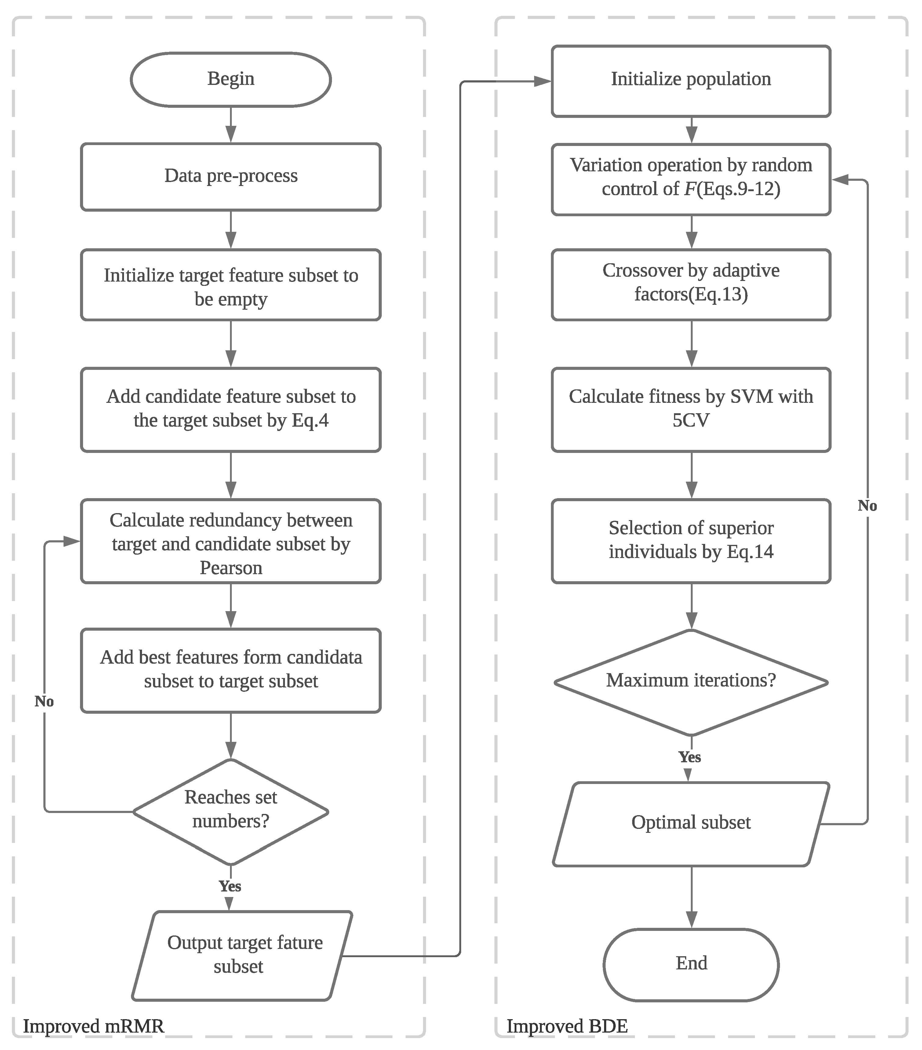
To address these limitations, we propose the MBDE algorithm. This approach utilizes the mRMR method to capture the correlations between features and updates the quantization function to handle continuous attributes. Furthermore, the BDE method is employed for fine-scale feature selection. The general workflow of the proposed method is illustrated in Figure 1. It can be divided into three stages.

In the first stage, the data are preprocessed, which includes handling missing values and performing data normalization. In the second stage, an improved mRMR algorithm is employed for initial feature filtering, resulting in the retention of 500 features in our experimental setup. Finally, in the third stage, the improved BDE algorithm is utilized for further feature selection, ultimately outputting the best subset of features. By integrating these stages, the proposed method aims to effectively address the challenges of feature selection in microarray data analysis, considering both the attribute continuity and the interdependence among genes.

3.2. Stage One: Preprocessing Method

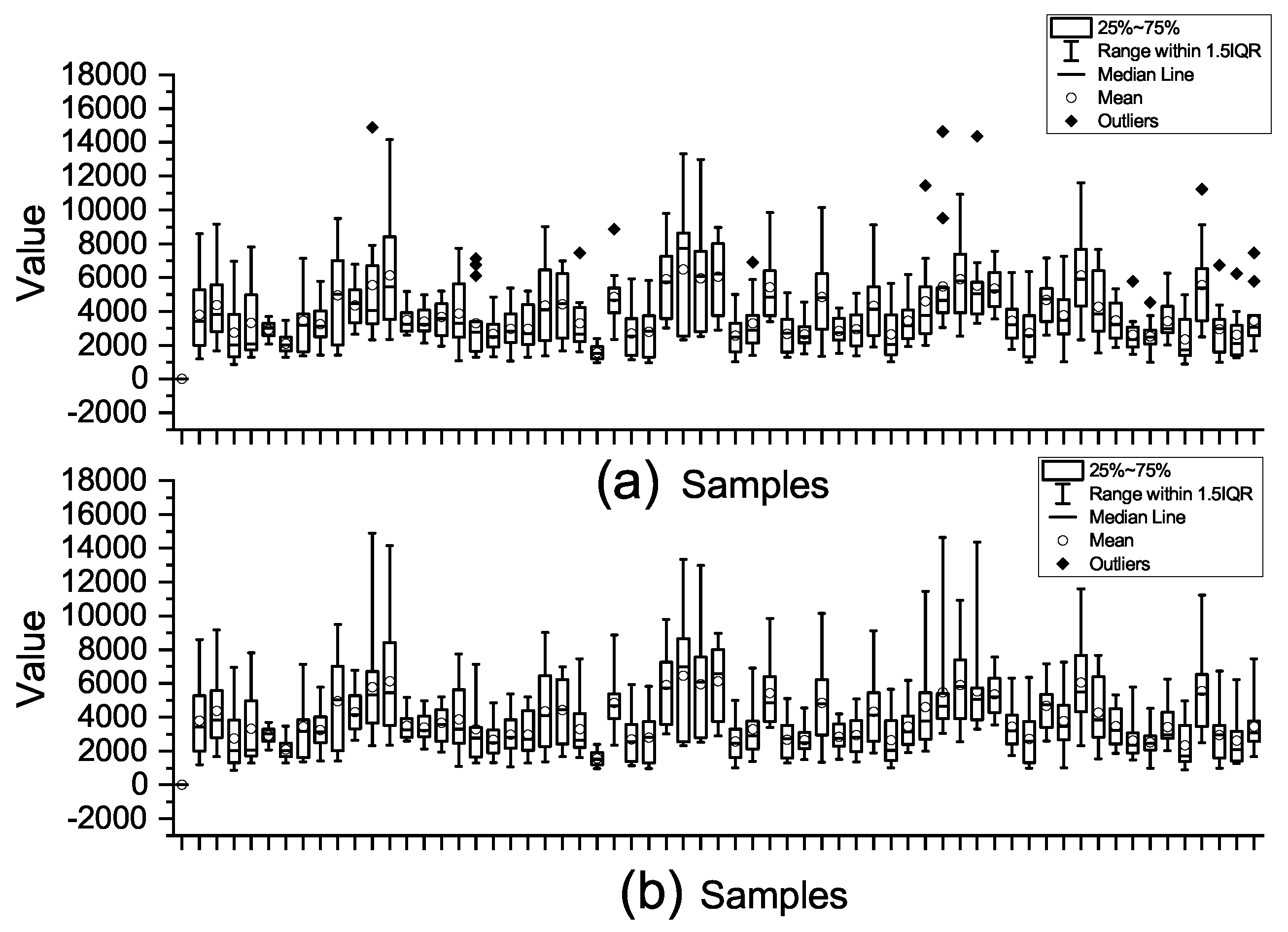
The original dataset contains outliers and missing values, which can negatively impact the data quality and subsequent analysis. To address this issue, we apply the $3\sigma$ principle to identify outliers in the data. Specifically, we consider data points outside the range of $(\mu -3\sigma ,\mu +3\sigma )$ as outliers, where $\mu$ represents the mean and $\sigma$ represents the standard deviation.

To handle both outliers and missing values, we employ the K-nearest neighbors (KNN) imputation method. This approach fills in the missing values and replaces outliers with values derived from neighboring data points. By using KNN, we can ensure that the imputed values are representative of the local data distribution. Furthermore, we apply a logarithmic transformation to all expressed data. This transformation helps to reveal data relationships more effectively and facilitates better statistical inference.

To illustrate the effect of the preprocessing steps, Figure 2 shows the impact of outlier and missing value processing by using the Colon dataset as an example. As observed, the preprocessing steps effectively remove outliers and prepare the dataset for subsequent analysis and tasks.

3.3. Stage Two: Improved mRMR Algorithm

In the context of microarray data analysis, the dimensionality of the data is typically high. Applying the wrapper method directly to select features would result in a significant increase in the algorithm complexity. Therefore, it is common to use a filter method for coarse-scale feature selection initially. One effective filtering feature-selection method is the Minimum Redundancy Maximum Relevance (mRMR) algorithm. The mRMR algorithm is an incremental search algorithm that aims to select features with the highest correlation to the target variable while minimizing redundancy with the already-selected features.

Traditionally, the mRMR algorithm employs two objectives for feature selection: maximizing the relevance between the features and the target variable, and minimizing the redundancy among the selected features. These objectives are mathematically described by Equation (1) and Equation (2), respectively:

$$maxA(S,C)=\frac{1}{n}\sum _{f_i\in S}I\left(f_i;C\right)$$

(1)

$$minR\left(S\right)=\frac{1}{n^2}\sum _{f_i,f_j\in S}I\left(f_i;f_j\right)$$

(2)

In Equations (1) and (2), S represents the feature subset, C represents the label variable, and $f_i$ and $f_j$ represent features within the feature subset S. The term $A(S,C)$ denotes the correlation between the target feature subset S and the label C, while $R\left(S\right)$ represents the redundancy within the feature subset S.

In the traditional mRMR algorithm, the correlation and redundancy are quantitatively calculated by using mutual information. The mutual information between two variables X and Y is mathematically represented by Equation (3):

$$I(\mathrm{X};\mathrm{Y})={\int }_X{\int }_{Y}P(X,Y)log\frac{P(X,Y)}{P\left(X\right)P\left(Y\right)}$$

(3)

In Equation (3), $P(X,Y)$ represents the joint probability distribution of the random variables X and Y, while $P\left(X\right)$ and $P\left(Y\right)$ represent their respective marginal probability distributions.

The traditional mRMR algorithm incorporates the two objective functions, Equations (1) and (2), into the feature-selection process. There are two common methods of integration: subtractive integration and divisive integration. This paper adopts the subtractive integration approach.

While the traditional mRMR algorithm utilizes mutual information to quantify the relationships between features and between features and labels, applying mutual information to microarray data poses challenges, as it is more suitable for data with continuous attributes and may require expert guidance for the binning operation. In contrast, the t-test and Pearson correlation coefficient are not subject to such limitations and have demonstrated superior performance in feature-selection tasks for microarray data [23]. The equations for the t-test and Pearson correlation coefficient are described in Equation (4) and Equation (5), respectively:

$$t\left(f_i\right)=\frac{\left|{\overline{f}}_{i_{pos}}-{\overline{f}}_{i_{neg}}\right|}{\sqrt{S_{i_{pos}}^2/n_{pos}+S_{i_{neg}}^2/n_{neg}}}$$

(4)

$$\rho \left(f_i,f_j\right)=\frac{\sum \left(f_i-{\overline{f}}_i\right)\left(f_j-{\overline{f}}_j\right)}{\sqrt{\sum {\left(f_i-{\overline{f}}_i\right)}^2\sum {\left(f_j-{\overline{f}}_j\right)}^2}}$$

(5)

In Equation (4), ${\overline{f}}_{i_{pos}}$ represents the mean value of feature $f_i$ in the positive samples, while ${\overline{f}}_{i_{neg}}$ represents the mean value of feature $f_i$ in the negative samples. $S_{i_{pos}}^2$ and $S_{i_{neg}}^2$ denote the variances of feature $f_i$ in the positive and negative samples, respectively. $n_{pos}$ and $n_{neg}$ represent the number of samples in the positive and negative classes, respectively.

Considering a dataset with all features denoted as F and the subset of features to be selected as $F_S$, the search process of mRMR involves iteratively selecting the optimal features from the candidate feature subset $F-F_S$ and adding them to $F_S$. The selection conditions for the optimal features can be obtained by using Equation (6):

$$\underset{f_i\in F-F_s}{max}\left[t\left(f_i\right)-\frac{1}{s}{\sum }_{f_j\in F_s}\rho \left(f_i,f_j\right)\right]$$

(6)

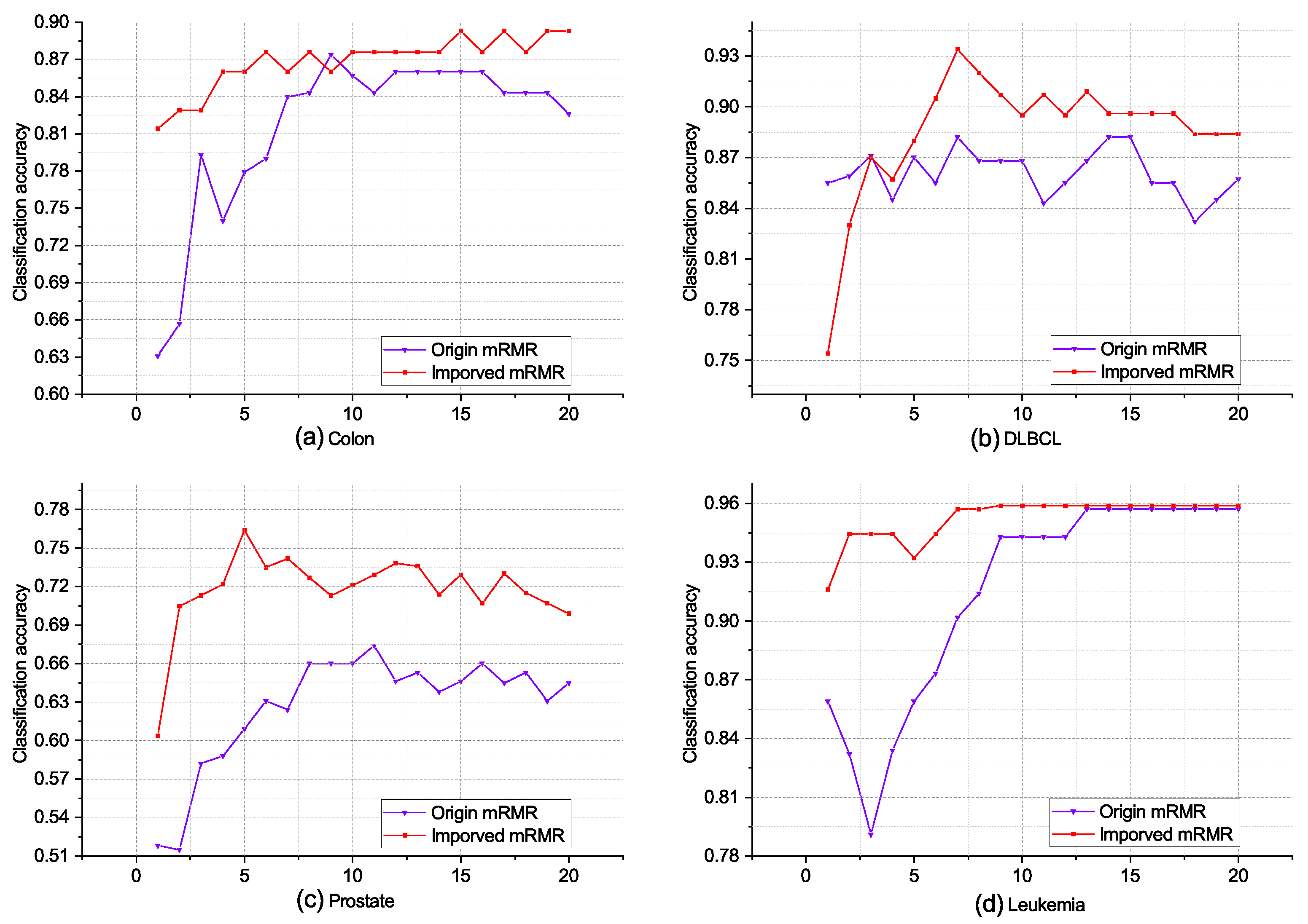
The original mRMR algorithm utilizes a predetermined number of features as the stopping criterion for the feature subset search. However, this criterion is determined empirically and may not guarantee optimal performance for the final feature subset selection. In this paper, we propose a modified stopping criterion for mRMR based on the average classification accuracy (Acc) of the classification model by using five-fold cross-validation on the current feature subset. The calculation of Acc is given by Equation (7), where $TP$ represents the number of true positive samples that are correctly predicted; $TN$ represents the number of true negative samples that are correctly predicted; and $FN$ and $FP$ represent the number of false negative and false positive predictions, respectively:

$$Acc=\frac{TP+TN}{TP+TN+FP+FN}$$

(7)

In this paper, we introduce a modified stopping criterion for the incremental search process in the mRMR algorithm. The criterion is considered to be met in the current case if either the classification accuracy of the classification model reaches 100% during the total search process or if there is no improvement observed for k consecutive iterations. This criterion ensures that the search process is terminated when the algorithm achieves an optimal classification performance or when further iterations do not yield significant improvements.

Moreover, the improved mRMR algorithm incorporates a quantization function suitable for continuous data to evaluate the correlation and redundancy between features. By applying this algorithm to microarray data, we can effectively filter out redundant, irrelevant, or weakly correlated genes. As a result, we obtain a subset of candidate biomarkers from the complete set of genes, which enhances the efficiency and relevance of the feature-selection process for microarray data analysis.

3.4. Stage Three: Improved BDE Algorithm

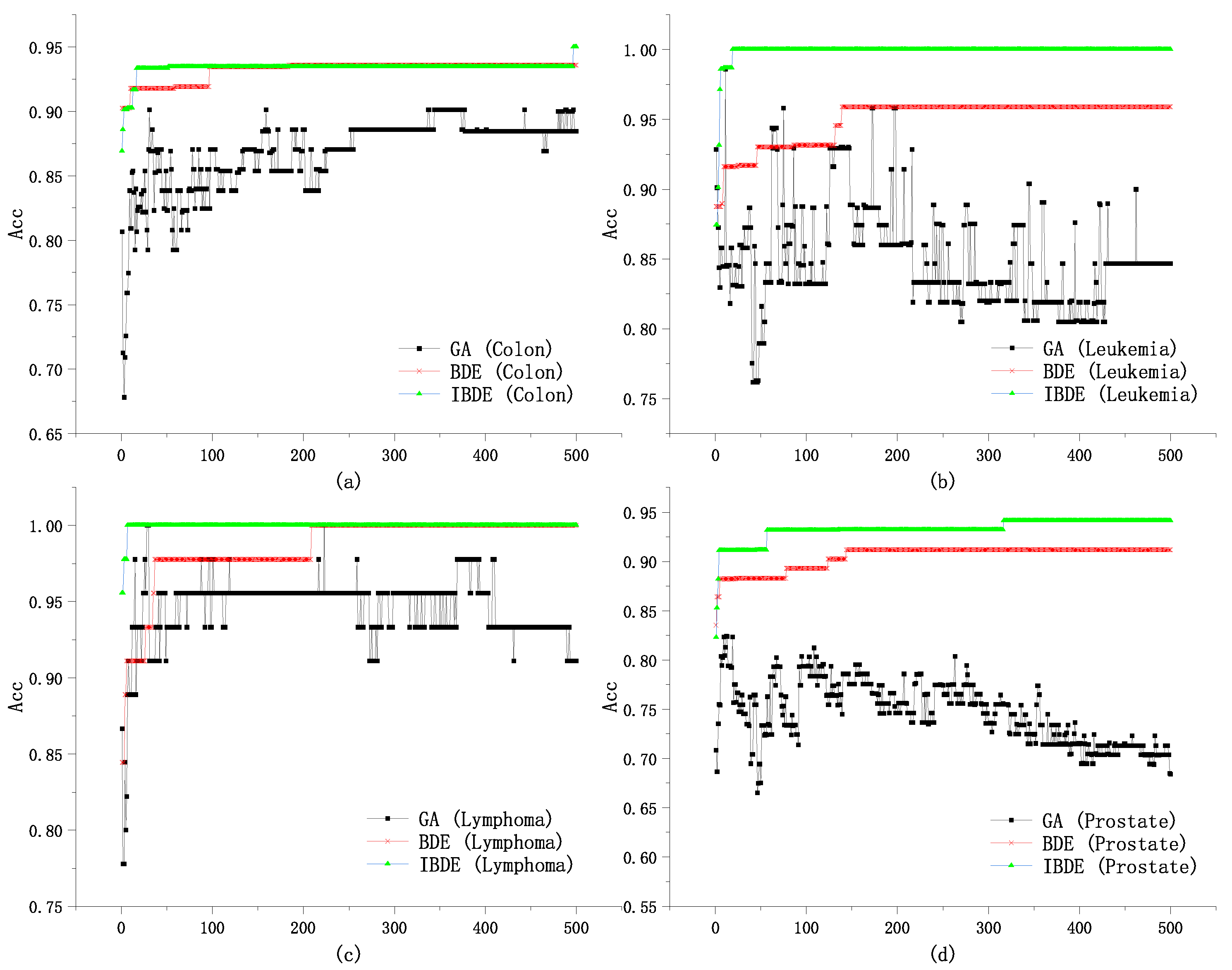
The proposed approach in this subsection introduces an improved binary differential evolution (DE) algorithm specifically designed for feature selection in microarray data analysis. DE is a widely utilized adaptive global optimization algorithm known for its simplicity, ease of implementation, rapid convergence, and robustness. It has found applications in various domains including data mining, pattern recognition, and artificial neural networks.

In our work, we enhance the DE algorithm by incorporating a new binary quantization method and scaling factor. This extension aims to enhance the algorithm’s exploration capability in the initial stage, thus improving population diversity. Additionally, we ensure the algorithm’s exploitation capability in the subsequent stage to exploit local advantages. To achieve this, we introduce an adaptive crossover operator, which not only accelerates the convergence speed in the initial stage but also maintains the algorithm’s exploitation capability in later stages.

The improved binary differential evolution algorithm presented in this paper addresses the challenges of feature-selection in microarray data by effectively balancing exploration and exploitation. This enhancement allows for the more efficient and accurate identification of relevant features for microarray analysis, contributing to the overall performance and effectiveness of the feature-selection process.

The traditional binary differential evolution algorithm calculates the variance vector $H_i\left(g\right)$ through the evolution process, as described in Equation (8). In this equation, three individuals $X_{p1}$, $X_{p2}$, and $X_{p3}$ are randomly chosen from the population, with the condition $i\ne p1\ne p2\ne p3$:

$$H_i\left(g\right)=X_{p1}\left(g\right)+F·\left(X_{p2}\left(g\right)-X_{p3}\left(g\right)\right)$$

(8)

However, this direct manipulation of the binary strings in the traditional approach does not effectively emulate the behavior of the continuous differential evolution algorithm. Consequently, it exhibits suboptimal performance, particularly in scenarios involving high-dimensional data [24].

Therefore, in the improved binary difference evolution algorithm, we use the vector $u_i\left(g\right)$ to represent the j-th binary code of the final mutation vector, which is shown as Equation (9):

$$u_i^j\left(g\right)=\left\{\begin{array}{c}1, \mathrm{if} pr\ge \mathrm{rand} (0,1) \mathrm{or} X_{p3}^j\left(g\right)=1\\ 0, \mathrm{otherwise} \end{array}\right.$$

(9)

In Equation (9), the value of $pr$ is calculated according to Equation (10) to ensure that the vector approximation after binary quantization falls within the range of 0 to 1. The proposed binary quantization method was inspired by [25]. In this method, when F is set to 0.5, $pr$ is approximately 0.462, and when F is set to 1, $pr$ is approximately 0.762. This implies that in Equation (9), even if F is 1, it will not cause $pr$ to exceed the value of rand (0, 1), thereby reducing the likelihood of selecting the j-th feature. As a result, the number of features is effectively reduced:

$$pr=\frac{e^{{\mathrm{diff}}_i^j\left(g\right)}-e^{-{\mathrm{diff}}_i^j\left(g\right)}}{e^{{\mathrm{diff}}_i^j\left(g\right)}+e^{-{\mathrm{diff}}_i^j\left(g\right)}}$$

(10)

The ${diff}_i^j\left(g\right)$ represents the j-th dimension binary code of the difference vector, which is calculated in Equation (11):

$$\mathrm{diff}{ }_i^j\left(g\right)=\left\{\begin{array}{c}0, \mathrm{if} X_{p1}^j\left(g\right)=X_{p2}^j\left(g\right)\hfill \\ F{X}_i^j\left(g\right), \mathrm{otherwise} \hfill \end{array}\right.$$

(11)

The scaling factor F plays a crucial role in balancing exploration and exploitation in the improved BDE algorithm. Increasing the value of F helps expand the search range and enhance population diversity, thereby promoting exploration. On the other hand, decreasing the value of F improves the exploitation ability and accelerates convergence, but may lead to premature convergence.

In the improved BDE algorithm, the value of F is determined based on Equation (12), where g represents the current iteration number and G represents the total number of iterations. By incorporating the iteration information, the scaling factor F dynamically adjusts over the course of the algorithm. Moreover, in the selection of $X_{p1}$, we ensure that $X_{p1}$ and $X_{p2}$ are not equal, preserving the element of randomness. This improved scaling factor strategy effectively strikes a balance between exploration and exploitation in the algorithm:

$$F=\left\{\begin{array}{c} \mathrm{rand} [0,0.5],(g/G)\ge 0.5\hfill \\ \mathrm{rand} [0.5,1],(g/G)<0.5\hfill \end{array}\right.$$

(12)

The crossover process plays a crucial role in maintaining population diversity in the improved BDE algorithm. The improved adaptive crossover operator is computed according to Equation (13), where $\alpha$ represents a parameter that will be further discussed in the experimental section. The final selection operator is determined based on Equation (14). In our method, we utilize the support vector machine (SVM) as the model to calculate the fitness function.

The adaptive crossover operator, as described in Equation (13), adjusts the crossover probability based on the fitness value of the individual. This allows individuals with higher fitness values to have a higher probability of undergoing crossover, while individuals with lower fitness values have a lower probability. By adaptively adjusting the crossover probability, the algorithm can effectively balance exploration and exploitation, promoting the convergence of the population toward better solutions.

In our method, the fitness function is evaluated by using the support vector machine (SVM) model. The SVM is a popular and effective classifier that can distinguish between positive and negative samples based on the selected features. The fitness function quantifies the classification accuracy of the SVM model, guiding the search process toward selecting features that contribute to a better classification performance:

$$CR=\alpha \frac{2e^{-(g/G)}}{e^{(g/G)}+e^{-(g/G)}}$$

(13)

$$x_i(g+1)=\left\{\begin{array}{cc}{v}_i\left(g\right)\hfill & , \mathrm{if} f\left(v_i\left(g\right)\right) \mathrm{better} \mathrm{than} f\left(x_i\left(g\right)\right)\hfill \\ x_i\left(g\right)\hfill & , \mathrm{otherwise} \hfill \end{array}\right.$$

(14)

where $x_i(g+1)$ is a new individual and $f(🞶)$ is the average classification accuracy of SVM five-fold cross-validation.

4. Experimental Results

4.1. The Results of Improved mRMR

In order to demonstrate that the improved mRMR algorithm can better rank important features when evaluating features, and thus more important features can be selected for further analysis when performing feature filtering, we selected the top 20 features by using the traditional mRMR algorithm and the improved mRMR algorithm, respectively, and compared these features in turn by using the average classification accuracy of ten-fold cross-validation as the evaluation metric. In the comparison, we sequentially added features to the test set for testing, using Gaussian Naive Bayes as the classifier.

Figure 3 depicts the results of the comparison experiments utilizing the Gaussian Naive Bayes classifier. In the comparison experiments conducted on the Colon dataset, the classification accuracy of the improved mRMR algorithm exhibited a marginal decrease relative to the original mRMR algorithm when the number of selected features was set at nine. However, for other configurations of selected features, the improved mRMR algorithm showcased superior classification accuracy over its original counterpart. Notably, the improved mRMR algorithm achieved a peak classification accuracy of approximately 89.3% when employing 15 selected features. In contrast, the original mRMR algorithm attained its maximum classification accuracy of approximately 87.4% when nine features were selected. These findings substantiate the superiority of the improved mRMR algorithm in terms of the classification accuracy on the Colon dataset.

In the comparison experiments conducted on the DLBCL dataset, the performance of the original mRMR algorithm and the improved mRMR algorithm varied based on the number of selected features. Initially, when a small number of features was selected, the original mRMR algorithm outperformed the improved mRMR algorithm. However, as the number of features increased to four, the improved mRMR algorithm gradually surpassed the original mRMR algorithm in terms of classification accuracy. Notably, the improved mRMR algorithm achieved a peak classification accuracy of approximately 93.4% when seven features were selected. In comparison, the original mRMR algorithm attained a maximum classification accuracy of about 88.2%.

In the comparison experiments conducted on the Leukemia dataset, the improved mRMR algorithm consistently outperformed the original mRMR algorithm in terms of the classification accuracy across the entire range of selected features, from 1 to 20. The advantage of the improved algorithm was particularly evident when a small number of features was selected, and its superiority gradually diminished as the number of features increased. Notably, the improved mRMR algorithm achieved a peak classification accuracy of approximately 95.9% when nine features were selected. In contrast, the original mRMR algorithm attained its highest classification accuracy of 95.7% when 13 features were selected.

In the comparison experiments conducted on the Prostate dataset, the improved mRMR algorithm consistently outperformed the original mRMR algorithm in terms of the classification accuracy across the entire range of selected features, from 1 to 20. The advantage of the improved algorithm was particularly evident when a small number of features was selected. Notably, the improved mRMR algorithm achieved its highest classification accuracy of approximately 76.4% when five features were selected. In contrast, the original mRMR algorithm attained its highest classification accuracy of about 67.4% when 11 features were selected.

It can be seen from Figure 3 that the classification accuracy does not increase with the increase in the number of selected features. For example, in the comparison experiments on the Leukemia dataset, the classification accuracy of the original mRMR algorithm and the improved mRMR algorithm first increased and then stabilized with the increase in the number of features. At the same time, in the comparison experiments on the Prostate dataset, the classification accuracy first increased and then decreased with the increase in the number of features. In the comparison experiment on the Prostate dataset, the classification accuracy tended to increase and then decrease with the number of features. This trend is because as the number of selected features increases, irrelevant, redundant, and noisy features are added to the target feature subset, resulting in a decrease in the classification accuracy, so it is important to reduce the dimensionality of such high-dimensional data as feature microarray data.

4.2. The Results of Improved BDE

In this subsection, we evaluate the effectiveness of the improved binary differential evolution algorithm by comparing it with two other algorithms: the classical genetic algorithm and the binary differential evolution algorithm. The comparison is performed by using a set of 500 features that have been filtered by the improved mRMR method. All the algorithms are configured with identical parameter settings, and the number of iterations is set to 500. Figure 4 presents the fitness variation of the different algorithms over the course of the iterations on the four datasets.

The results depicted in Figure 4 demonstrate the distinctive characteristics of the three algorithms. The genetic algorithm exhibits continuously changing fitness values throughout the iterations and tends to achieve lower fitness values after convergence. It is particularly challenging for the genetic algorithm to converge, as observed in the case of the Prostate dataset. Due to its nature of altering individuals through crossover operations, ensuring the survival of the best individuals becomes challenging. Consequently, the genetic algorithm is not well-suited for handling high-dimensional data with limited samples. On the other hand, both the binary differential evolution (BDE) and improved binary differential evolution (IBDE) algorithms perform exceptionally well in convergence scenarios. They converge rapidly on all datasets, ensuring high classification accuracy rates. Although BDE slightly outperforms IBDE in terms of the classification accuracy, it lacks a clear criterion for limiting the number of features selected.

Table 3. The best fitness (classification accuracy) versus number of features for the three algorithms.

	GA		BDE		IBDE
Datasets	Features	Acc	Features	Acc	Features	Acc
Colon	16	0.9012	54	0.9500	7	0.9358
Leukemia	12	0.9857	67	1.0000	7	0.9590
Prostate	10	0.8242	57	0.9414	7	0.9119
Lymphoma	20	1.0000	59	1.0000	7	1.0000
DLBCL	17	0.9244	49	0.9583	6	0.9667
Gastric	12	0.9087	55	0.9328	6	0.9449
Stroke	15	0.9385	42	0.9725	4	0.9670
ALL1	10	1.0000	45	1.0000	2	1.0000

provides detailed information regarding the number of features and the corresponding classification accuracy achieved after convergence by each algorithm.

The results presented in Table 3 reveal interesting findings. While the average classification accuracy achieved by the IBDE algorithm is approximately 0.008 lower than that of the BDE algorithm across the eight datasets, it is noteworthy that the average number of features selected by the BDE algorithm is 9.3 times higher than that of the IBDE algorithm. This suggests that the BDE algorithm is able to significantly reduce the number of features while maintaining a satisfactory classification accuracy.

4.3. Parameter Analysis

In this subsection, we delve into the analysis of the parameter in the IBDE algorithm.

Table 4. The parameter analysis of MBDE.

Paramenter	Dataset	Features	Acc	Time Cost(s)
$\alpha =0.9$	Colon	4	0.9333	2657.5594
	Leukemia	6	0.9723	2794.3365
	Prostate	4	0.9119	2870.0474
	Lymphoma	5	0.9777	2740.1594
$\alpha =0.7$	Colon	3	0.9179	2685.4997
	Leukemia	5	0.9304	2796.2625
	Prostate	3	0.8933	2898.1710
	Lymphoma	3	0.9777	2725.0789
$\alpha =0.5$	Colon	5	0.9666	2671.4259
	Leukemia	10	0.9714	2839.8899
	Prostate	10	0.9123	2896.5553
	Lymphoma	2	0.9777	2731.6164
$\alpha =0.3$	Colon	7	0.9358	2598.0236
	Leukemia	7	0.9590	2872.5760
	Prostate	7	0.9119	2895.0205
	Lymphoma	7	1.0000	2755.2378

presents the number of features retained and the fitness of the algorithm under different parameter settings. It is evident that when the parameter $\alpha$ is set to a small value, the algorithm exhibits a stronger search capability, resulting in better fitness. However, this leads to a larger number of retained features. Conversely, when the parameter $\alpha$ is increased, the algorithm tends to retain fewer features. Nevertheless, the fitness is not noticeably compromised. Hence, the parameter $\alpha$ can be adjusted based on specific application requirements to strike a balance between classification accuracy and the number of features. Furthermore, it is worth noting that the parameters do not have a significant impact on the time complexity of the algorithm.

4.4. Comparison with Classical Feature-Selection Methods

In this subsection, we conduct a comprehensive comparison between the proposed methods and classical feature-selection algorithms. To ensure fair and unbiased results, all methods employ Support Vector Machine (SVM) as the classifier, and the average classification accuracy from five-fold cross-validation is utilized as the final evaluation metric. Moreover, the number of features used in the compared methods is kept consistent for a meaningful comparison.

The classical feature-selection algorithms considered in this comparison include L1 regularization (Lasso), random forest (RF), logistic regression (LR), L2 regularization (Ridge), correlation coefficient (Corr), decision tree (DT), mutual information (MIC), independent sample t-test (t-test), and stability selection (Stab). The corresponding results are summarized in

Table 5. Results of comparison with classical feature-selection methods on Acc, bold indicates the best result.

Datasets	Lasso	RF	LR	Ridge	Corr	DT	MIC	t-test	Stab	Proposed
Colon	0.921	0.946	0.913	0.920	0.931	0.921	0.906	0.844	0.933	0.935
Leukemia	0.893	0.921	0.917	0.910	0.933	0.920	0.881	0.823	0.911	0.959
Prostate	0.881	0.890	0.786	0.911	0.822	0.885	0.853	0.797	0.906	0.911
Lymphoma	0.988	0.973	0.973	0.950	0.946	0.958	0.897	0.871	0.990	1.000
DLBCL	0.943	0.943	0.937	0.961	0.937	0.958	0.912	0.887	0.943	0.966
Gastric	0.911	0.934	0.922	0.822	0.900	0.925	0.857	0.863	0.933	0.944
Stroke	0.895	0.885	0.843	0.887	0.935	0.903	0.857	0.813	0.938	0.967
ALL1	1.000	1.000	1.000	1.000	1.000	1.000	0.967	0.955	1.000	1.000

.

Table 5 clearly demonstrates the superiority of the proposed methods over the classical feature-selection algorithms across all datasets. Notably, the proposed method achieves substantial improvements in classification accuracy compared to the classical algorithms. On average, the proposed method outperforms the classical feature-selection algorithms by 2.23% on the Colon dataset, 6.40% on the Leukemia dataset, 6.11% on the Prostate dataset, 5.17% on the Lymphoma dataset, 3.27% on the DLBCL dataset, 5.38% on the Gastric dataset, 9.32% on the Stroke dataset, and 0.86% on the ALL1 dataset. These results clearly demonstrate the effectiveness of the proposed method in improving the classification accuracy compared to the classical approaches.

To further demonstrate the sophistication of the proposed method, we also compared two evaluation metrics, precision and recall, with detailed results shown in

Table 6. Results of comparison with classical feature-selection methods on Precision, bold indicates the best result.

Datasets	Lasso	RF	LR	Ridge	Corr	DT	MIC	t-test	Stab	Proposed
Colon	0.863	0.873	0.956	0.924	0.924	0.924	0.956	0.924	0.782	0.927
Leukemia	0.933	0.933	1.000	0.933	0.933	0.927	0.933	0.670	0.656	0.944
Prostate	0.960	0.960	0.913	0.978	0.960	0.960	0.978	0.942	0.831	0.988
Lymphoma	0.983	0.974	0.843	0.988	0.979	0.960	0.960	0.960	0.705	1.000
DLBCL	0.883	0.883	0.960	0.960	0.860	0.824	0.960	0.883	0.694	0.976
Gastric	0.769	0.769	0.931	0.927	0.971	0.967	0.967	0.931	0.672	0.955
Stroke	0.860	0.820	0.817	0.762	0.900	0.736	0.867	0.808	0.750	0.988
ALL1	1.000	1.000	0.975	1.000	1.000	1.000	1.000	1.000	1.000	1.000

and

Table 7. Results of comparison with classical feature-selection methods on Recall, bold indicates the best result.

Datasets	Lasso	RF	LR	Ridge	Corr	DT	MIC	t-test	Stab	Proposed
Colon	0.925	0.900	1.000	0.875	0.925	0.925	0.925	0.925	0.900	0.945
Leukemia	0.920	0.920	0.720	0.960	0.960	0.920	1.000	0.600	0.741	0.942
Prostate	0.922	0.922	0.940	0.867	0.885	0.885	0.849	0.885	0.607	0.978
Lymphoma	0.960	0.960	0.870	0.910	0.910	0.910	0.960	0.910	0.860	1.000
DLBCL	0.800	0.800	0.800	1.000	0.950	0.950	1.000	0.850	0.855	0.956
Gastric	0.977	0.967	0.893	0.927	0.927	0.893	0.860	0.893	0.827	0.961
Stroke	0.800	0.800	0.700	0.995	0.989	0.900	0.850	0.976	0.855	0.977
ALL1	1.000	1.000	1.000	1.000	1.000	1.000	1.000	1.000	1.000	1.000

. It can be seen that the proposed method equally outperforms all traditional feature-selection methods, with an average improvement of 8.02% and 7.46% across all datasets for both evaluation metrics.

4.5. Compare with Hybrid Feature-Selection Method

This subsection presents a comparison between the proposed method and several advanced hybrid feature-selection methods, with detailed results provided in

Table 8. Comparison of MBDE and other hybrid methods.

Datasets	Methods	Acc	Features
Colon	Gao [12]	0.9032	3.0
	Sun [13]	0.8430	5.0
	Lu [3]	0.8909	19.0
	Wang [14]	0.8570	11.1
	Lu [15]	0.8400	3.0
	Vanitha [27]	0.7419	3.0
	Proposed	0.9333	4.0
Leukemia	Aziz [26]	0.9868	12.0
	Tumuluru [28]	0.9459	NAN
	Sun [13]	0.9273	3.0
	Lu [3]	0.9762	7.0
	Wang [14]	0.9610	8.3
	Lu [15]	0.9520	9.0
	Proposed	0.9723	6.0
Prostate	Canedo [29]	0.9060	25.0
	Jinthanasatian [30]	0.8743	5.0
	Wu [31]	0.9044	NAN
	Wang [14]	0.9040	9.0
	Lu [15]	0.9160	4.0
	Proposed	0.9119	4.0
Lymphoma	Moradi [32]	0.8771	50.0
	Vanitha [27]	0.9090	4.0
	Proposed	0.9777	5.0

. The analysis reveals that the proposed method achieves superior performance on the Colon, Prostate, and Lymphoma datasets compared to the existing methods. Specifically, the proposed method achieves a higher classification accuracy while utilizing a smaller number of features. Although the classification accuracy of the MBDE method is slightly lower than that of the method proposed by Aziz et al. [26] on the Leukemia dataset, the proposed method still demonstrates its advanced nature by reducing the number of selected features by six. Overall, these results highlight the effectiveness and competitiveness of the proposed method when compared to the existing approaches.

4.6. Model Overfitting Analysis

In this section, we analyze the risk of overfitting of the model. Specifically, we established an external test dataset on the dataset, which includes 30% of the original data samples, and then used the remaining 70% of the data for five-fold cross-validation to train the model. Then, we used the remaining 30% of the data to test different evaluation metrics. We also provided the model’s predicted TP, FP, FN, and TN, where TP (true positive) refers to the number of positive samples correctly predicted by the model, FP (false positive) refers to the number of negative samples incorrectly predicted as positive, TN (true negative) refers to the number of negative samples correctly predicted, and FN (false negative) refers to the number of positive samples incorrectly predicted as negative.

We compared these results with the model’s five-fold cross-validation results on all the data, where TP, FP, FN, and TN count the total in different test processes of the cross-validation, and the other results are averaged. Considering the limitation of data sample size, we conducted experiments on the CESC and LIHC datasets. The detailed results are shown in

Table 9. Five-fold cross-validation results on all datasets and independent test data validation results.

	5-Fold Cross-Validation		Test Set Evaluation
Evaluation Metrics	CESC	LIHC	CESC	LIHC
TP	53.000	72.000	62.000	87.000
FP	20.000	21.000	8.000	12.000
FN	48.000	68.000	12.000	15.000
TN	186.000	262.000	10.000	13.000
Acc	0.779	0.790	0.793	0.787
Recall	0.525	0.514	0.552	0.512
Precision	0.726	0.774	0.727	0.786

. The results from Table 9 show that the model has similar performance in the five-fold cross-validation results and the independent test set, thus indicating good control over the risk of overfitting.

To further illustrate the detailed results of our method on different datasets and to demonstrate the model’s reliability in predicting different classes of samples, as well as to show that the model does not risk overfitting, we have also compiled the confusion matrices for all datasets. The results, shown in

Table 10. Confusion matrix of experimental results.

Datasets	TP	FP	FN	TN
Colon	38	2	2	20
Leukemia	44	3	3	22
Prostate	49	3	2	48
Lymphoma	22	0	0	23
DLBCL	56	2	2	17
Gastric	28	1	1	35
Stroke	19	1	1	19
ALL1	95	0	0	33
CESC	53	20	48	186
LIHC	72	21	68	262

, indicate that the model has a good capability in predicting samples, including some imbalanced samples.

To further demonstrate that our model has a low risk of overfitting and exhibits a good predictive performance on most datasets, we calculated the random predictive performance, Acc_random, and the improvement of the model over this random performance for each dataset. This calculation was performed according to the method described in the literature [33,34] and by using Equations (15) and (16). The specific results are presented in

Table 11. Performance improvement ratio of the model over random prediction for different datasets.

Datasets	Acc_random	$\Delta$Accuracy (%)
Colon	0.54	39.33
Leukemia	0.55	37.00
Prostate	0.50	45.10
Lymphoma	0.50	49.98
DLBCL	0.63	31.98
Gastric	0.51	46.34
Stroke	0.50	45.00
ALL1	0.62	38.27
CESC	0.59	18.88
LIHC	0.59	19.49

. It is evident that our model performs well across all microarray data. For RNA-seq data, the results are lower, which is a common issue. The range of results from classic feature-selection methods on this dataset is as follows (CESC: 0.71–0.75, LIHC: 0.70–0.74). Currently, researchers are widely adopting multiomics integration techniques for these types of data to enhance performance, as evaluated in references [35,36,37]. Therefore, overall, our model is effective in disease diagnosis and prediction and carries a low risk of overfitting:

$$\mathrm{Acc}\_\mathrm{random}=\frac{(TP+FN)(TP+FP)+(TN+FN)(TN+FP)}{N^2}$$

(15)

$$\Delta \mathrm{Accuracy}=\mathrm{Acc}-\mathrm{Acc}\_\mathrm{random}$$

(16)

4.7. Analysis of the Features Selected by the Proposed Method

In this subsection, we conducted a statistical analysis on the features selected by the proposed method to determine their potential as biomarkers. To illustrate this analysis, we present the results for the first four features from the Leukemia and Prostate datasets.

Table 12. Information on the selected features of the proposed method. PubMed Hits indicate the number of articles after searching with that gene name and disease name as keywords, *** represents p < 0.001, and t-test was used as the calculation.

Datasets	Prob ID	Gene Name	PubMed Hits	p-Value
Leukemia	M15395_at	ITGB2	8	***
	U23852_s_at	LCK	266	***
	D28473_s_at	IARS	1	***
	M54992_at	CD72	32	***
Prostate	858_at	POR	506	***
	34376_at	PKIG	0	***
	38291_at	PENK	7	***
	914_g_at	ERG	1453	***

provides the probe IDs of these features, along with the corresponding gene names obtained through ID-to-name conversion by using the GPL platform. The “PubMed Hits” column indicates the number of search results in PubMed when querying the disease name along with the gene name, which serves as an indicator of whether the gene has been reported to be associated with the disease. The p-value represents the statistical significance obtained from conducting an independent sample t-test. A p-value less than 0.001 is denoted by ***.

The results presented in Table 12 demonstrate that the majority of features selected by the proposed method have corresponding entries in PubMed, indicating their reported association with the respective diseases. This further validates the diagnostic significance of the selected features.

For the Leukemia dataset, the independent samples t-test revealed the following findings: In the ITGB2 group, the “Neg” values were significantly lower than the mean of the “Pos” values, with a statistically significant difference of −2.115 (−2.875 to −1.355) between the two groups (p< 0.001). In the LCK group, the “Neg” values were higher than the mean of the “Pos” values, with a difference of 1.381 (0.619 to 2.143), and the difference was statistically significant (p < 0.001). In the IARS group, the “Neg” values were higher than the mean of the “Pos” values, with a difference of 0.699 (0.309 to 1.09), and the difference was statistically significant (p < 0.001). In the CD72 group, the “Neg” values were higher than the mean of the “Pos” values, with a difference of 1.348 (0.698 to 1.998), and the difference was statistically significant (p < 0.001).

For the Prostate dataset, the independent samples t-test yielded the following observations: In the POR group, the “Neg” values were higher than the mean of the “Pos” values, with a statistically significant difference of 0.108 (0.026 to 0.189) between the two groups (p < 0.001). In the PKIG group, the “Neg” values were lower than the mean of the “Pos” values, with a difference of −0.228 (−0.41 to −0.046), and the difference was statistically significant (p < 0.001). In the PENK group, the “Neg” values were lower than the mean of the “Pos” values, with a difference of −0.918 (−1.174 to −0.662) between the two groups, and the difference was statistically significant (p < 0.001). In the ERG group, the “Neg” values were higher than the mean of the “Pos” values, with a difference of 1.132 (0.796 to 1.468), and the difference was statistically significant (p < 0.001).

These findings indicate that the selected features are statistically significant in distinguishing between different classes and have the potential to serve as biomarkers for the respective diseases.

We also performed a heat map analysis the expression of these four genes in positive and negative samples, and the results are shown in Figure 5. We found differences in the distribution of samples between positive and negative samples, demonstrating that the genes selected by the proposed method are able to distinguish between positive and negative samples.

To further analyze the ability of the selected features to discriminate between samples on the whole, we used PCA to downscale the above four features to obtain three dimensions and visualized the ability of the downscaled information to discriminate between positive and negative samples by using 3D visualization techniques, and the results are shown in Figure 6. The black sample points in the figure represent Pos samples and the red sample points represent Neg samples. We can see that the features selected by the proposed method can effectively distinguish between different samples and have the potential ability to diagnose diseases.

Figure 7 presents the correlation analysis of the features selected by the proposed method, utilizing the Pearson correlation coefficient as a measure. The Prostate dataset reveals that none of the selected features exhibit a significant correlation. Conversely, the Leukemia dataset demonstrates a significant correlation within a specific group of features. The absence of significant correlations among the remaining features further supports the efficacy of the proposed method, highlighting its ability to select nonredundant features. In summary, the features selected by the proposed method exhibit low redundancy, as evidenced by the correlation analysis.

5. Conclusions

This paper presents a hybrid feature-selection algorithm that integrates an improved mRMR method with an enhanced binary differential evolution algorithm for microarray data analysis. By refining the quantization functions, this method boosts the capability of mRMR to handle continuous attributes and conducts coarse-scale feature filtering. Subsequently, the enhanced binary differential evolution algorithm is applied for fine-scale feature selection. The algorithm, augmented with an adaptive crossover operator, effectively reduces the number of features while balancing the exploration and exploitation capabilities. The experimental results demonstrate that the proposed approach successfully decreases feature dimensionality and selects biomarkers with high accuracy and diagnostic significance, which are crucial for disease diagnosis and prevention.

However, there are limitations to the approach presented in this study. Although the improved binary differential evolution algorithm shows promise in feature selection, the single-objective evolutionary algorithm still faces challenges in balancing classification accuracy with the number of features, especially when dealing with complex datasets. Moreover, while the introduction of an adaptive crossover operator enhances the flexibility in exploring the feature space, there is room for improvement in global search capabilities and the guidance of elite solution sets. Future research might explore more intricate multiobjective optimization strategies or introduce more efficient global search mechanisms to overcome these limitations and further enhance the performance and practicality of the algorithm.

References

1. Zhang, J.; Xu, D.; Hao, K.; Zhang, Y.; Chen, W.; Liu, J.; Gao, R.; Wu, C.; De Marinis, Y. FS–GBDT: Identification multicancer-risk module via a feature selection algorithm by integrating Fisher score and GBDT. Briefings Bioinform. 2020, 22, bbaa189. [Google Scholar] [CrossRef]
2. Chaudhuri, A.; Sahu, T.P. A hybrid feature selection method based on Binary Jaya algorithm for micro-array data classification. Comput. Electr. Eng. 2021, 90, 106963. [Google Scholar] [CrossRef]
3. Lu, H.; Chen, J.; Yan, K.; Jin, Q.; Xue, Y.; Gao, Z. A hybrid feature selection algorithm for gene expression data classification. Neurocomputing 2017, 256, 56–62. [Google Scholar] [CrossRef]
4. Salem, H.; Attiya, G.; El-Fishawy, N. Classification of human cancer diseases by gene expression profiles. Appl. Soft Comput. 2017, 50, 124–134. [Google Scholar] [CrossRef]
5. Kononenko, I.; Šimec, E.; Robnik-Šikonja, M. Overcoming the myopia of inductive learning algorithms with RELIEFF. Appl. Intell. 1997, 7, 39–55. [Google Scholar] [CrossRef]
6. Zhou, N.; Wang, L. A modified T-test feature selection method and its application on the HapMap genotype data. Genom. Proteom. Bioinform. 2007, 5, 242–249. [Google Scholar] [CrossRef] [PubMed]
7. Liu, H.; Setiono, R. Chi2: Feature selection and discretization of numeric attributes. In Proceedings of the 7th IEEE International Conference on Tools with Artificial Intelligence, Herndon, VA, USA, 5–8 November 1995; pp. 388–391. [Google Scholar]
8. Yan, K.; Zhang, D. Feature selection and analysis on correlated gas sensor data with recursive feature elimination. Sens. Actuators B Chem. 2015, 212, 353–363. [Google Scholar] [CrossRef]
9. Li, X.; Xiao, N.; Claramunt, C.; Lin, H. Initialization strategies to enhancing the performance of genetic algorithms for the p-median problem. Comput. Ind. Eng. 2011, 61, 1024–1034. [Google Scholar] [CrossRef]
10. Yan, X.; Nazmi, S.; Erol, B.A.; Homaifar, A.; Gebru, B.; Tunstel, E. An efficient unsupervised feature selection procedure through feature clustering. Pattern Recognit. Lett. 2020, 131, 277–284. [Google Scholar] [CrossRef]
11. Chen, K.H.; Wang, K.J.; Tsai, M.L.; Wang, K.M.; Adrian, A.M.; Cheng, W.C.; Yang, T.S.; Teng, N.C.; Tan, K.P.; Chang, K.S. Gene selection for cancer identification: A decision tree model empowered by particle swarm optimization algorithm. BMC Bioinform. 2014, 15, 49. [Google Scholar] [CrossRef]
12. Gao, L.; Ye, M.; Lu, X.; Huang, D. Hybrid Method Based on Information Gain and Support Vector Machine for Gene Selection in Cancer Classification. Genom. Proteom. Bioinform. 2017, 15, 389–395. [Google Scholar] [CrossRef] [PubMed]
13. Sun, L.; Zhang, X.Y.; Qian, Y.H.; Xu, J.C.; Zhang, S.G.; Tian, Y. Joint neighborhood entropy-based gene selection method with fisher score for tumor classification. Appl. Intell. 2018, 49. [Google Scholar] [CrossRef]
14. Wang, A.; An, N.; Yang, J.; Chen, G.; Li, L.; Alterovitz, G. Wrapper-based gene selection with Markov blanket. Comput. Biol. Med. 2017, 81, 11–23. [Google Scholar] [CrossRef]
15. Lin, S.; Xz, A.; Yq, C.; Jx, A.; Sz, A. Feature selection using neighborhood entropy-based uncertainty measures for gene expression data classification. Inf. Sci. 2019, 502, 18–41. [Google Scholar]
16. Xie, W.; Wang, L.; Yu, K.; Shi, T.; Li, W. Improved multi-layer binary firefly algorithm for optimizing feature selection and classification of microarray data. Biomed. Signal Process. Control 2023, 79, 104080. [Google Scholar] [CrossRef]
17. Xie, W.; Li, W.; Zhang, S.; Wang, L.; Yang, J.; Zhao, D. A novel biomarker selection method combining graph neural network and gene relationships applied to microarray data. BMC Bioinform. 2022, 23, 303. [Google Scholar] [CrossRef]
18. Karakaya, G.; Galelli, S.; Ahipaşaoğlu, S.D.; Taormina, R. Identifying (quasi) equally informative subsets in feature selection problems for classification: A max-relevance min-redundancy approach. IEEE Trans. Cybern. 2015, 46, 1424–1437. [Google Scholar] [CrossRef] [PubMed]
19. Xiu, Y.; Zhao, S.; Chen, H.; Li, C. I-mRMR: Incremental Max-Relevance, and Min-Redundancy Feature Selection. In Proceedings of the Asia-Pacific Web (APWeb) and Web-Age Information Management (WAIM) Joint International Conference on Web and Big Data, Chengdu, China, 1–3 August 2019; pp. 103–110. [Google Scholar]
20. Pant, M.; Zaheer, H.; Garcia-Hernandez, L.; Abraham, A. Differential Evolution: A review of more than two decades of research. Eng. Appl. Artif. Intell. 2020, 90, 103479. [Google Scholar]
21. Gao, S.; Wang, K.; Tao, S.; Jin, T.; Dai, H.; Cheng, J. A state-of-the-art differential evolution algorithm for parameter estimation of solar photovoltaic models. Energy Convers. Manag. 2021, 230, 113784. [Google Scholar] [CrossRef]
22. A new hybrid wrapper TLBO and SA with SVM approach for gene expression data. Inf. Sci. 2019, 503, 238–254. [CrossRef]
23. Alsalem, M.; Zaidan, A.; Zaidan, B.; Hashim, M.; Madhloom, H.; Azeez, N.; Alsyisuf, S. A review of the automated detection and classification of acute leukaemia: Coherent taxonomy, datasets, validation and performance measurements, motivation, open challenges and recommendations. Comput. Methods Programs Biomed. 2018, 158, 93–112. [Google Scholar] [CrossRef]
24. Chen, Y.; Xie, W.; Zou, X. A binary differential evolution algorithm learning from explored solutions. Neurocomputing 2015, 149, 1038–1047. [Google Scholar] [CrossRef]
25. Deng, C.; Zhao, B.; Yang, Y.; Zhang, H. Binary encoding differential evolution for combinatorial optimization problems. Int. J. Educ. Manag. Eng. 2011, 1, 59–66. [Google Scholar] [CrossRef]
26. Aziz, R.; Verma, C.K.; Srivastava, N. A Novel Approach for Dimension Reduction of Microarray. Comput. Biol. Chem. 2017, 71, 161–169. [Google Scholar] [CrossRef]
27. Vanitha, C.; Devaraj, D.; Venkatesulu, M. Gene Expression Data Classification Using Support Vector Machine and Mutual Information-based Gene Selection. Procedia Comput. Sci. 2015, 47, 13–21. [Google Scholar] [CrossRef]
28. Tumuluru, P.; Ravi, B. GOA-based DBN: Grasshopper optimization algorithm-based deep belief neural networks for cancer classification. Int. J. Appl. Eng. Res. 2017, 12, 14218–14231. [Google Scholar]
29. Bolón-Canedo, V.; Sánchez-Maroño, N.; Alonso-Betanzos, A. An ensemble of filters and classifiers for microarray data classification. Pattern Recognit. 2012, 45, 531–539. [Google Scholar] [CrossRef]
30. Jinthanasatian, P.; Auephanwiriyakul, S.; Theera-Umpon, N. Microarray data classification using neuro-fuzzy classifier with firefly algorithm. In Proceedings of the 2017 IEEE Symposium Series on Computational Intelligence (SSCI), Honolulu, HI, USA, 27 November–1 December 2017. [Google Scholar]
31. Wu, S.J.; Pham, V.H.; Nguyen, T.N. Two-phase Optimization for Support Vectors and Parameter Selection of Support Vector Machines: Two-class Classification. Appl. Soft Comput. 2017, 59, 129–142. [Google Scholar] [CrossRef]
32. Moradi, P.; Gholampour, M. A hybrid particle swarm optimization for feature subset selection by integrating a novel local search strategy. Appl. Soft Comput. 2016, 43, 117–130. [Google Scholar] [CrossRef]
33. Lučić, B.; Batista, J.; Bojović, V.; Lovrić, M.; Sović Kržić, A.; Bešlo, D.; Nadramija, D.; Vikić-Topić, D. Estimation of random accuracy and its use in validation of predictive quality of classification models within predictive challenges. Croat. Chem. Acta 2019, 92, 379–391. [Google Scholar] [CrossRef]
34. Batista, J.; Vikić-Topić, D.; Lučić, B. The difference between the accuracy of real and the corresponding random model is a useful parameter for validation of two-state classification model quality. Croat. Chem. Acta 2016, 89, 527–534. [Google Scholar] [CrossRef]
35. Wang, T.; Shao, W.; Huang, Z.; Tang, H.; Zhang, J.; Ding, Z.; Huang, K. MOGONET integrates multi-omics data using graph convolutional networks allowing patient classification and biomarker identification. Nat. Commun. 2021, 12, 3445. [Google Scholar] [CrossRef] [PubMed]
36. Cantini, L.; Zakeri, P.; Hernandez, C.; Naldi, A.; Thieffry, D.; Remy, E.; Baudot, A. Benchmarking joint multi-omics dimensionality reduction approaches for the study of cancer. Nat. Commun. 2021, 12, 124. [Google Scholar] [CrossRef] [PubMed]
37. Poirion, O.B.; Jing, Z.; Chaudhary, K.; Huang, S.; Garmire, L.X. DeepProg: An ensemble of deep-learning and machine-learning models for prognosis prediction using multi-omics data. Genome Med. 2021, 13, 112. [Google Scholar] [CrossRef] [PubMed]
Figure 1. Overall process of MBDE algorithm.
Processes 12 00313 g001
Figure 2. The effect of outlier and missing value processing on the Colon dataset (only part of the data are shown), (a) is before data preprocessing and (b) is after data preprocessing.
Processes 12 00313 g002
Figure 3. In the comparison experiments between the original mRMR algorithm and the improved mRMR algorithm, the horizontal axis represents the number of selected features while the plain Bayes classifier is used for classification. Among the 80 sets of comparison experiments conducted on the four datasets, a total of 76 sets, accounting for 95% of the experimental results, demonstrate that the improved mRMR algorithm achieves higher classification accuracy compared to the original mRMR algorithm.
Processes 12 00313 g003
Figure 4. The variation in fitness with respect to the number of iterations for the improved binary differential evolution algorithm, the traditional binary differential evolution algorithm, and the genetic algorithm across different datasets. (a) represents the results of the Colon dataset, (b) represents the results of the Leukemia dataset, (c) represents the results of the Lymphoma dataset and (d) represents the results of the Prostate dataset.
Processes 12 00313 g004
Figure 5. Heat map of Leukemia and Prostate, with sample cut-off line indicating the split between Pos samples and Neg samples.
Processes 12 00313 g005
Figure 6. The 3D visualization of the features selected by the proposed method. The black sample points in the figure represent Pos samples and the red sample points represent Neg samples. The percentages of the different axes in the figure indicate the percentage of the original feature information that is represented by that principal component.
Processes 12 00313 g006
Figure 7. Correlation analysis of the features selected by the proposed method, with Pearson correlation coefficients.
Processes 12 00313 g007